Max-Sum Diversification, Monotone Submodular Functions and Dynamic Updates

Abstract

Result diversification is an important aspect in web-based search, document summarization, facility location, portfolio management and other applications. Given a set of ranked results for a set of objects (e.g. web documents, facilities, etc.) with a distance between any pair, the goal is to select a subset $S$ satisfying the following three criteria: (a) the subset $S$ satisfies some constraint (e.g. bounded cardinality); (b) the subset contains results of high “quality”; and (c) the subset contains results that are “diverse” relative to the distance measure. The goal of result diversification is to produce a diversified subset while maintaining high quality as much as possible. We study a broad class of problems where the distances are a metric, where the constraint is given by independence in a matroid, where quality is determined by a monotone submodular function, and diversity is defined as the sum of distances between objects in $S$. Our problem is a generalization of the max sum diversification problem studied in [3] which in turn is a generalization of the max sum $p$-dispersion problem studied extensively in location theory. It is NP-hard even with the triangle inequality. We propose two simple and natural algorithms: a greedy algorithm for a cardinality constraint and a local search algorithm for an arbitrary matroid constraint. We prove that both algorithms achieve constant approximation ratios.

1 Introduction

Result diversification has many important applications in databases, operations research, information retrieval, and finance. In this paper, we study and extend a particular version of result diversification, known as max-sum diversification. More specifically, we consider the setting where we are given a set of elements in a metric space and a set valuation function $f$ defined on every subset. For any given subset $S$, the overall objective is a linear combination of $f(S)$ and the sum of the distances induced by $S$. The goal is to find a subset $S$ satisfying some constraints that maximizes the overall objective.

This diversification problem is first studied by Gollapudi and Sharma in [3] for modular (i.e. linear) set functions and for sets satisfying a cardinality constraint (i.e. a uniform matroid). (See [3] for some closely related work.) The max-sum $p$-dispersion problem seeks to find a subset $S$ of cardinality $p$ so as to maximize $\sum_{x,y\in S}d(x,y)$. The diversification problem is then a linear combination of a quality function $f()$ and the max-sum dispersion function. Gollapudi and Sharma give a 2 approximation greedy algorithm for some metrical distance diversification problems by reducing to the analogous dispersion problem. More specifically for max-sum diversification they use the greedy algorithm of Hassin, Rubsenstein and Tamir [4]. Hassin et al give a non greedy algorithm for a more general problem where the goal is to construct $k$ subsets each having $p$ elements. (We willl restrict attention to the case $k=1$.) Their non greedy algorithm obtains the ratio $2-\frac{1}{\lceil p/2\rceil}$ and hence the same approximation holds for the Gollapudi and Sharma diversification problem.

The first part of our paper considers an extension of the modular case to the monotone submodular case, for which the algorithm in [3] no longer applies. We are able to maintain the same 2-approximation using a natural, but different greedy algorithm. We then further extend the problem by considering any matroid constraint and show that a natural single swap local search algorithm provides a 2-approximation in this more general setting. This extends the Nemhauser, Wolsey and Fisher [5] approximation result for the problem of submodular function maximization subject to a matroid constraint (without the distance function component). We note that the dispersion function is a supermodular function and hence the Nemhauser er al result does not immediately extend to our diversification problem.

Submodular functions have been extensively considered since they model many natural phenomena. For example, in terms of keyword based search in database systems, it is well understood that users begin to gradually (or sometimes abruptly) lose interest the more results they have to consider [7, 8]. But on the other hand, as long as a user continues to gain some benefit, additional query results can improve the overall quality but at a decreasing rate. In a related application, Lin and Bilnes [9] argue that monotone submodular functions are an ideal class of functions for text summarization. Following and extending the results in [3], we consider the case of maximizing a linear combination of a submodular quality function $f(S)$ and the max-sum dispersion subject to a cardinality constraint (i.e., $|S|\leq p$ for some given $p$). We present a greedy algorithm that is somewhat unusual in that it does not try to optimize the objective in each iteration but rather optimizes a closely related potential function. We show that our greedy approach matches the greedy $2$-approximation in [3] obtained for diversification with a modular quality function. We note that the greedy algorithm in [3] utilizes the max dispersion algorithm of Hassin, Rubinstein and Tamir [4] which greedily adds edges whereas our algorithm greedily adds vertices.

Our next result continues with the submodular case but now we go beyond a cardinality constraint (i.e., the uniform matroid) on $S$ and allow the constraint to be that $S$ is independent in a given matroid. This allows a substantial increase in generality. For example, while diversity might represented by the distance between retrieved database tuples under a given criterion (for instance, a kernel based diversity measure called answer tree kernel is used in [10]), we could use a partition matroid to insure that (for example) the retrieved database tuples come from a variety of different sources. That is, we may wish to have $n_{i}$ tuples from a specific database field $i$. This is, of course, another form of diversity but one orthogonal to diversity based on the given criterion. Similarly in the stock portfolio example, we might wish to have a balance of stocks in terms of say risk and profit profiles (using some statistical measure of distances) while using a submodular quality function to reflect a users submodular utility for profit and using a partition matroid to insure that different sectors of the economy are well represented. Another important class of matroids (relevant to the above applications) is that of transversal matroids. Suppose we have a collection $\{C_{1},C_{2},\ldots,C_{m}$} of (possibly) overlapping sets (i.e., the collection is not necessarily a partition) of database tuples (or stocks). Our goal might be to derive a set $S$ such that the database tuples in $S$ form a set of representatives for the collection; that is, every database tuple in $S$ represents (and is in) a unique set $C_{i}$ in the collection. The set $S$ is then an independent set in the transversal matroid induced by the collection. We also note [11] that the intersection of any matroid with a uniform matroid is still a matroid so that in the above examples, we could further impose the constraint that the set S has at most $p$ elements.

Our final theoretical result concerns dynamic updates. Here we restrict attention to a modular set function $f(S)$; that is, we now have weights on the elements and $f(S)=\sum_{u\in S}w(u)$ where $w(u)$ is the weight of element $u$. This allows us to consider changes to the weight of a single element as well as changes to the distance function.

The rest of the paper is organized as follows. In Section 2, we discuss related work in dispersion and result diversification. In Section 3, we formulate the problem as a combinatorial optimization problem and discuss the complexity of the problem. In Section 4, we consider max-sum diversification with monotone submodular set quality functions subject to a cardinality constriant and give a conceptually simple greedy algorithm that achieves a 2-approximation. We extend the problem to the matroid case in Section 5 and discuss dynamic updates in Section 6. Section 7 carries out a number of experiments. In particular, we compare our greedy algorithm with the greedy algorithm of Gollapudi and Sharma. Section 8 concludes the paper.

2 Related Work

With the proliferation of today’s social media, database and web content, ranking becomes an important problem as it decides what gets selected and what does not, and what to be displayed first and what to be displayed last. Many early ranking algorithms, for example in web search, are based on the notion of “relevance”, i.e., the closeness of the object to the search query. However, there has been a rising interest to incorporate some notion of “diversity” into measures of quality.

One early work in this direction is the notion of “Maximal Marginal Relevance” (MMR) introduced by Carbonell and Goldstein in [12]. More specifically, MMR is defined as follows:

$${\rm MMR}=\max_{D_{i}\in R\setminus S}[\lambda\cdot sim_{1}(D_{i},Q)-(1-\lambda)\max_{D_{j}\in S}sim_{2}(D_{i},D_{j})],$$

where $Q$ is a query; $R$ is the ranked list of documents retrieved; $S$ is the subset of documents in $R$ already selected; $sim_{1}$ is the similarity measure between a document and a query, and $sim_{2}$ is the similarity measure between two documents. The parameter $\lambda$ controls the trade-off between novelty (a notion of diversity) and relevance. The MMR algorithm iteratively selects the next document with respect to the MMR objective function until a given cardinality condition is met. The MMR heuristic has been widely used, but to the best of our knowledge, it has not been theoretically justified. Our paper provides some theoretical evidence why MMR is a legitimate approach for diversification. The greedy algorithm we propose in this paper can be viewed as a natural extension of MMR.

There is extensive research on how to diversify returned ranking results to satisfy multiple users. Namely, the result diversity issue occurs when many facets of queries are discovered and a set of multiple users expect to find their desired facets in the first page of the results. Thus, the challenge is to find the best strategy for ordering the results such that many users would find their relevant pages in the top few slots.

Rafiei et al. [13] modeled this as a continuous optimization problem. They introduce a weight vector $W$ for the search results, where the total weight sums to one. They define the portfolio variance to be $W^{T}CW$, where $C$ is the covariance matrix of the result set. The goal then is to minimize the portfolio variance while the expected relevance is fixed at a certain level. They report that their proposed algorithm can improve upon Google in terms of the diversity on random queries, retrieving $14\%$ to $38\%$ more aspects of queries in top five, while maintaining a precision very close to Google.

Bansal et al. [14] considered the setting in which various types of users exist and each is interested in a subset of the search results. They use a performance measure based on discounted cumulative gain, which defines the usefulness (gain) of a document as its position in the resulting list. Based on this measure, they suggest a general approach to develop approximation algorithms for ranking search results that captures different aspects of users’ intents. They also take into account that the relevance of one document cannot be treated independent of the relevance of other documents in a collection returned by a search engine. They consider both the scenario where users are interested in only a single search result (e.g., navigational queries) and the scenario where users have different requirements on the number of search results, and develop good approximation solutions for them.

The database community has recently studied the query diversification problem, which is mainly for keyword search in databases [15, 16, 17, 8, 10, 7, 18]. Given a very large database, an exploratory query can easily lead to a vast answer set. Typically, an answer’s relevance to the user query is based on top-k or tf-idf. As a way of increasing user satisfaction, different query diversification techniques have been proposed including some system based ones taking into account query parameters, evaluation algorithms, and dataset properties. For many of these, a max-sum type objective function is usually used.

Other than those discussed above, there are many recent papers studying result diversification in different settings, via different approaches and through different perspectives, for example [19, 20, 21, 22, 23, 24, 25, 26, 27, 28]. The reader is referred to [24, 29] for a good summary of the field. Most relevant to our work is the paper by Gollapudi and Sharma [3], where they develop an axiomatic approach to characterize and design diversification systems. Furthermore, they consider three different diversification objectives and using earlier results in facility dispersion, they are able to give algorithms with good worst case approximation guarantees. This paper is a continuation of research along this line.

Recently, Minack et al. [30] have studied the problem of incremental diversification for very large data sets. Instead of viewing the input of the problem as a set, they consider the input as a stream, and use a simple online algorithm to process each element in an incremental fashion, maintaining a near-optimal diverse set at any point in the stream. Although their results are largely experimental, this approach significantly reduces CPU and memory consumption, and hence is applicable to large data sets. Our dynamic update algorithm deals with a problem of a similar nature, but in addition to our experimental results, we are also able to prove theoretical guarantees. To the best of our knowledge, our work is the first of its kind to obtain a near-optimality condition for result diversification in a dynamically changing environment.

Independent of our conference paper [31], Abbassi, Mirrokni and Thakus [32] have also shown that the (Hamming distance 1) local search algorithm provides a 2-approximation for the max-sum dispersion problem subject to a matroid constraint. Their version of the dispersion problem is somwehat more general in that they additionally consider that the points are chosen from different clusters. They indirectly consider a quality measure by first restricting the universe of objects to high quality objects and then apply dispersion. They provide a number of interesting experimental results.

3 Problem Formulation

Although the notion of “diversity” naturally arises in the context of databases, social media and web search, the underlying mathematical object is not new. As presented in [3], there is a rich and long line of research in location theory dealing with a similar concept; in particular, one objective is the placement of facilities on a network to maximize some function of the distances between facilities. The situation arises when proximity of facilities is undesirable, for example, the distribution of business franchises in a city. Such location problems are often referred to as dispersion problems; for more motivation and early work, see [33, 34, 35].

Analytical models for the dispersion problem assume that the given network is represented by a set $V=\{v_{1},v_{2},\dots,v_{n}\}$ of $n$ vertices along with a distance function between every pair of vertices. The objective is to locate $p$ facilities ($p\leq n$) among the $n$ vertices, with at most one facility per vertex, such that some function of distances between facilities is maximized. Different objective functions are considered for the dispersion problems in the literature including: the max-sum criterion (maximize the total distances between all pairs of facilities) in [36, 33, 37], the max-min criterion (maximize the minimum distance between a pair of facilities) in [35, 33, 37], the max-mst (maximize the minimum spanning tree among all facilities) and many other related criteria in [38, 39]. When the distances are arbitrary, the max-sum problem is a weighted generaliztion of the densest subgraph problem which is a known difficult problem not admitting a PTAS ([40] and not known to have a constant approximation algorithm. Sometimes the problem is studied for specific metric distances (e.g as in Fekete and Meijer [41]) or for restricted classes of weights (e.g. as in Czygrinow [42]) where there can be a PTAS.

Our diversification problem is a generalization of the max sum $p$-dispersion problem assuming arbitrary metric distances. For the max-sum criteria and for most of the objective criteria, the dispersion problem is NP-hard, and approximation algorithms have been developed and studied; see [39] for a summary of known results. Our diversification problem is a generalization of the following max sum $p$-dispersion problem for arbitrary metric distances. Most relevant to this paper is the max-sum dispersion problem with metric distances.

Problem 1. Max-Sum $p$ Dispersion

Let $U$ be the underlying ground set, and let $d(\cdot,\cdot)$ be a metric distance function on $U$. Given a fixed integer $p$, the goal of the problem is to find a subset $S\subseteq U$ that:

$$\begin{array}[]{ll}\rm{maximizes}&\sum_{\{u,v\}:{u,v\in S}}d(u,v)\\ \\ \rm{subject\;\;to}&|S|=p,\end{array}$$

The problem is known to be NP-hard by an easy reduction from Max-Clique, and as noted by Alon [43], there is evidence that the problem is hard to compute in polynomial time with approximation $2-\epsilon$ for any $\epsilon>0$ when $p=n^{r}$ for $1/3\leq r<1$. Namely, based on the assumption that the planted clique problem is hard, Alon et al [45] show that it is hard to distinguish between a graph having a large planted clique of size $p$ and one in which the densest subgraph of size $p$ is of density at most an arbitrarily small constant $\delta$ (for suffiently large $n$). Considering the complement of a random graph $G$ in ${\cal G}(n,1/2)$, their result says that it is hard to distinguish between a graph having an independent set of size $p$ and one in which the density of edges in any size $p$-subgraph is at least $(1-\delta)$. Adding another node to the complement graph that is connected to all nodes in $G$, the graph distance metric is now the $\{1,2\}$ metric formed by the transitive closure so that adjacent nodes have distance 1 and non adjacent nodes have distance 2. So we therefore cannot distinguish between graphs where there exists a set of nodes $S$ of size $p$ ( for $p$ as above) where $\sum_{(u,v)\in S}d(u,v)={p\choose 2}*2$ and one where in every set of size $p$, we have $\sum_{(u,v)\in S}d(u,v)\leq{p\choose 2}[(1-\delta)+2\delta]$.

In [37], Ravi, Rosenkrantz and Tayi give a greedy algorithm (greedily choosing vertices that is shown to have approximation ratio no worse than $4$ and no better than $\frac{2}{1+2/p(p-1)}$. Hassin, Rubenstein and Tamir [4] improve upon the Ravi et al result by an algorithm that greedily chooses edges yielding an approximation ratio of $2$. Hassin et al also give an algorithm based on maximum matching that provides a $2-\frac{1}{\lceil p/2\rceil}$ approximation for a more general problem; namely, the algorithm must find a subset $U^{\prime}$ which is partitioned into $k$ disjoint subsets, each of size $p$ so as to maximize the pairwise sum of all pairs of vertices in $U^{\prime}$. The more general $(p,k)$ problem is similar to a partition matroid constraint but in a partition matroid, the partition is given as part of the definition of the matroid and each block of the partition has its own cardinality constraint.

Answering an open problem stated in Hassin et al., Birnbaum and Goldman [46] give an improved analysis proving that the Ravi et al greedy algorithm results in a $\frac{2p-2}{p-1}$ approximation for the max-sum $p$ dispersion problem. This then shows that a 2-approximation is a tight bound (as $p$ grows) for the Ravi et al greedy algorithm. More generally, Birnbaum and Goldman show that greedily choosing a set of $d$ nodes provides a $\frac{2p-2}{p+d-2}$ approximation. Our analysis in Section 4 yields an alternative proof that the Ravi et al greedy algorithm approximation ratio is no worse than $2$ even when extended to the max-sum $p$ diversification problem (with a monotone submodular value function) considered in Section 4.

Problem 2. Max-Sum $p$ Diversification

Let $U$ be the underlying ground set, and let $d(\cdot,\cdot)$ be a metric distance function on $U$. For any subset of $U$, let $f(\cdot)$ be a non-negative set function measuring the value of a subset. Given a fixed integer $p$, the goal of the problem is to find a subset $S\subseteq U$ that:

$$\begin{array}[]{ll}\rm{maximizes}&f(S)+\lambda\sum_{\{u,v\}:{u,v\in S}}d(u,v)\\ \\ \rm{subject\;\;to}&|S|=p,\end{array}$$

where $\lambda$ is a parameter specifying a desired trade-off between the two objectives.

The max-sum diversification problem is first proposed and studied in the context of result diversification in [3] , where the function $f(\cdot)$ is modular. In their paper, the value of $f(S)$ measures the relevance of a given subset to a search query, and the value $\sum_{\{u,v\}:{u,v\in S}}d(u,v)$ gives a diversity measure on $S$. The parameter $\lambda$ specifies a desired trade-off between diversity and relevance. They reduce the problem to the max-sum dispersion problem, and using an algorithm in [4], they obtain an approximation ratio of 2.

In this paper, we first study the problem with more general valuation functions;namely, normalized, monotone submodular set functions. For notational convenience, for any two sets $S$, $T$ and an element $e$, we write $S\cup\{e\}$ as $S+e$, $S\setminus\{e\}$ as $S-e$, $S\cup T$ as $S+T$, and $S\setminus T$ as $S-T$. A set function $f$ is normalized if $f(\emptyset)=0$. The function is monotone if for any $S,T\subseteq U$ and $S\subseteq T$,

$$f(S)\leq f(T).$$

It is submodular if for any $S,T\subseteq U$, $S\subseteq T$ with $u\in U$,

$$f(T+u)-f(T)\leq f(S+u)-f(S).$$

In the remainder of paper, all functions considered are normalized.

We proceed to our first contribution, a greedy algorithm (different than the one in [3]) that obtains a 2-approximation for monotone submodular set functions.

4 Submodular Functions

Submodular set functions can be characterized by the property of a decreasing marginal gain as the size of the set increases. As such, submodular functions are well-studied objects in economics, game theory and combinatorial optimization. More recently, submodular functions have attracted attention in many practical fields of computer science. For example, Kempe et al. [47] study the problem of selecting a set of most influential nodes to maximize the total information spread in a social network. They have shown that under two basic stochastic diffusion models, the expected influence of an initially chosen set is submodular, hence the problem admits a good approximation algorithm. In natural language processing, Lin and Bilmes [48, 49, 9] have studied a class of submodular functions for document summarization. These functions each combine two terms, one which encourages the summary to be representative of the corpus, and the other which positively rewards diversity. Their experimental results show that a greedy algorithm with the objective of maximizing these submodular functions outperforms the existing state-of-art results in both generic and query-focused document summarization.

Both of the above mentioned results are based on the fundamental work of Nemhauser, Wolsey and Fisher [5], which gave an $\frac{e}{e-1}$-approximation for maximizing monotone submodular set functions over a uniform matroid. This bound is now known to be tight even for a general matroid [50] whereas the greedy algorithm provides a 2-approximation for an arbitrary matroid (and a $k+1$-approximation for the intersection of $k$ matroids) as shown in [51]. Our max-sum diversification problem with monotone submodular set functions can be viewed as an extension of that problem: the objective function now not only contains a submodular part, but also has a super-modular part: the sum of distances.

Since the max-sum diversification problem with modular set functions studied in [3] admits a 2-approximation algorithm, it is natural to ask what approximation ratio is obtainable for the same problem with monotone submodular set functions. The Gollapudi and Sharma algorithm is based on the observation that the diversity function with modular set functions can be reduced to the max-sum $p$ dispersion problem by changing the metric. Namely, the reduction defines the metric $d^{\prime}(u,v)=w(u)+w(v)+2\lambda d(u,v)$. It is clear then that this reduction and then algorithm in [3] does not apply to the submodular case where elements do not have weights but rather only marginal weights. While this suggests that a greedy algorithm using marginal weights might apply (as we will show), this still requires a proof and in general one cannot expect the same approximation ratio. In what follows we assume (as is standard when considering submodular functions) access to an oracle for finding an element $u\in U-S$ that maximizes $f(S+u)-f(S)$. When $f$ is modular, this simply means accessing the element $u\in U-S$ having maximum weight.

Theorem 1.

There is a simple linear time greedy algorithm that achieves a 2-approximation for the max-sum diversification problem with monotone submodular set functions satisfying a cardinality constraint.

Before giving the proof of Theorem 1, we first introduce our notation. We extend the notion of distance function to sets. For disjoint subsets $S,T\subseteq U$, we let $d(S)=\sum_{\{u,v\}:{u,v\in S}}d(u,v)$, and $d(S,T)=\sum_{\{u,v\}:{u\in S,v\in T}}d(u,v)$.

Now we define various types of marginal gain. For any given subset $S\subseteq U$ and an element $u\in U-S$: let $\phi(S)$ be the value of the objective function, $d_{u}(S)=\sum_{v\in S}d(u,v)$ be the marginal gain on the distance, $f_{u}(S)=f(S+u)-f(S)$ be the marginal gain on the weight, and $\phi_{u}(S)=f_{u}(S)+\lambda d_{u}(S)$ be the total marginal gain on the objective function. Let $f^{\prime}_{u}(S)=\frac{1}{2}f_{u}(S)$, and $\phi^{\prime}_{u}(S)=f^{\prime}_{u}(S)+\lambda d_{u}(S)$. We consider the following simple greedy algorithm:

Greedy Algorithm

$S=\emptyset$
while $|S|<p$
      find $u\in U-S$ maximizing $\phi^{\prime}_{u}(S)$
      $S=S+u$
end while
return $S$

Note that the above greedy algorithm is “non-oblivious” (in the sense of [52]) as it is not selecting the next element with respect to the objective function $\phi(\cdot)$. This might be of an independent interest. We utilize the following lemma in [37].

Lemma 1.

Given a metric distance function $d(\cdot,\cdot)$, and two disjoint sets $X$ and $Y$, we have the following inequality: $(|X|-1)d(X,Y)\geq|Y|d(X).$

Now we are ready to prove Theorem 1.

Proof.

Let $O$ be the optimal solution, and $G$, the greedy solution at the end of the algorithm. Let $G_{i}$ be the greedy solution at the end of step $i$, $i<p$; and let $A=O\cap G_{i}$, $B=G_{i}-A$ and $C=O-A$. By lemma 1, we have the following three inequalities:

$$(|C|-1)d(B,C)\geq|B|d(C)$$ (1)

$$(|C|-1)d(A,C)\geq|A|d(C)$$ (2)

$$(|A|-1)d(A,C)\geq|C|d(A)$$ (3)

Furthermore, we have

$$d(A,C)+d(A)+d(C)=d(O)$$ (4)

Note that the algorithm clearly achieves the optimal solution if $p=1$. If $|C|=1$, then $i=p-1$ and $G_{i}\subset O$. Let $v$ be the element in $C$, and let $u$ be the element taken by the greedy algorithm in the next step, then $\phi^{\prime}_{u}(G_{i})\geq\phi^{\prime}_{v}(G_{i})$. Therefore, $\frac{1}{2}f_{u}(G_{i})+\lambda d_{u}(G_{i})\geq\frac{1}{2}f_{v}(G_{i})+\lambda d_{v}(G_{i}),$ which implies $\phi_{u}(G_{i})=f_{u}(G_{i})+\lambda d_{u}(G_{i})\geq\frac{1}{2}f_{u}(G_{i})+\lambda d_{u}(G_{i})$ $\geq\frac{1}{2}f_{v}(G_{i})+\lambda d_{v}(G_{i})\geq\frac{1}{2}\phi_{v}(G_{i})$ and hence $\phi(G)\geq\frac{1}{2}\phi(O)$.

Now we can assume that $p>1$ and $|C|>1$. We apply the following non-negative multipliers to equations (1), (2), (3), (4) and add them: $(1)*\frac{1}{|C|-1}+(2)*\frac{|C|-|B|}{p(|C|-1)}+(3)*\frac{i}{p(p-1)}+(4)*\frac{i|C|}{p(p-1)}$; we then have $d(A,C)+d(B,C)-\frac{i|C|(p-|C|)}{p(p-1)(|C|-1)}d(C)\geq\frac{i|C|}{p(p-1)}d(O).$ Since $p>|C|$, $d(C,G_{i})\geq\frac{i|C|}{p(p-1)}d(O).$ By submodularity and monotonicity of $f^{\prime}(\cdot)$, we have $\sum_{v\in C}f^{\prime}_{v}(G_{i})\geq f^{\prime}(C\cup G_{i})-f^{\prime}(G_{i})\geq f^{\prime}(O)-f^{\prime}(G).$ Therefore, $\sum_{v\in C}\phi^{\prime}_{v}(G_{i})=\sum_{v\in C}[f^{\prime}_{v}(G_{i})+\lambda d(\{v\},G_{i})]$ $=\sum_{v\in C}f^{\prime}_{v}(G_{i})+\lambda d(C,G_{i})\geq[f^{\prime}(O)-f^{\prime}(G)]+\frac{\lambda i|C|}{p(p-1)}d(O).$

Let $u_{i+1}$ be the element taken at step $(i+1)$, then we have $\phi^{\prime}_{u_{i+1}}(G_{i})\geq\frac{1}{p}[f^{\prime}(O)-f^{\prime}(G)]+\frac{\lambda i}{p(p-1)}d(O).$ Summing over all $i$ from $0$ to $p-1$, we have $\phi^{\prime}(G)=\sum_{i=0}^{p-1}\phi^{\prime}_{u_{i+1}}(G_{i})\geq[f^{\prime}(O)-f^{\prime}(G)]+\frac{\lambda}{2}d(O).$ Hence, $f^{\prime}(G)+\lambda d(G)\geq f^{\prime}(O)-f^{\prime}(G)+\frac{\lambda}{2}d(O),$ and $\phi(G)=f(G)+\lambda d(G)\geq\frac{1}{2}[f(O)+\lambda d(O)]=\frac{1}{2}\phi(O).$ This completes the proof. ∎

The greedy algorithm runs in time proportional to $p$ (for the $p$ iterations) times the cost of computing $\phi^{\prime}_{u}(S)$ for a given $u$ and $S$. When $f$ is modular, the time for updating $\phi^{\prime}_{u}(S)$ can be bounded by $O(n)$. Namely, each iteration costs $O(n)$ time (to search over all elements $u$ in $U\setminus S$) and update $\phi^{\prime}(S)$. Updating $f^{\prime}(S)$ is clearly $O(1)$ while naively updating $d_{u}(S)$ would take time $O(p)$. But as observed by Birnbaum and Goldman [46], $d_{u}(V^{\prime})$ can be maintained for all $V\setminus S$ within the same $O(n)$ needed to search $V^{\prime}$ so that updating $\phi^{\prime}(S)$ only costs time $O(1)$. Hence the total time is $O(np)$, linear in $n$ when $p$ is a constant.

Corollary 1.

The Ravi et al. [37] greedy algorithm for dispersion has approximation ratio no worse that 2.

Proof.

The identically zero function $f$ is monotone submodular and for this $f$, our greedy algorithm is precisely the dispersion algorithm of Ravi et al. ∎

We note that for the dispersion problem, Birnbaum and Goldman [46] show that their bound for the greedy algorithm is tight. In particular, for the greedy algorithm that adds one element at a time, the precise bound is $\frac{2p-2}{p-1}$.

5 Matroids and Local Search

Theorem 1 provides a 2-approximation for max-sum diversification when the set function is submodular and the set constraint is a cardinality constraint, i.e., a uniform matroid. It is natural to ask if the same approximation guarantee can be obtained for an arbitrary matroid. In this section, we show that the max-sum diversification problem with monotone submodular function admits a 2-approximation subject to a general matroid constraint.

Matroids are well studied objects in combinatorial optimization. A matroid $\cal M$ is a pair $<U,{\cal F}>$, where $U$ is a set of ground elements and $\cal F$ is a collection of subsets of $U$, called independent sets, with the following properties :

• Hereditary: The empty set is independent and if $S\in{\cal F}$ and $S^{\prime}\subset S$, then $S^{\prime}\in{\cal F}$.

• Augmentation: If $A,B\in{\cal F}$ and $|A|>|B|$, then $\exists e\in A-B$ such that $B\cup\{e\}\in{\cal F}$.

The maximal independent sets of a matroid are called bases of $\cal M$. Note that all bases have the same number of elements, and this number is called the rank of $\cal M$. The definition of a matroid captures the key notion of independence from linear algebra and extends that notion so as to apply to many combinatorial objects. We have already mentioned two classes of matroids relevant to our results, namely partition matroids and transversal matroids. In a partition matroid, the universe $U$ is partitioned into sets $S_{1},\ldots,S_{m}$ and the independent sets $S$ satisfy $S=\cup_{1\leq i\leq m}S_{i}$ with $|S_{i}|\leq k_{i}$ for some given bounds $k_{i}$ on each part of the partition. A uniform matroid is a special case of a partition matroid with $m=1$. In a transversal matroid, the universe $U$ is a union of (possibly) intersecting sets ${\cal C}=C_{1},\ldots,C_{m}$ and a set $S=\{s_{1},\ldots s_{r}\}\subseteq U$ is independent if there is an injective function $\phi$ from $S$ into ${\cal C}$ with say $\phi(s_{i})=C_{i}$ and $\phi(s_{i})\in C_{i}$.That is, $S$ forms a set of representatives for each set $C_{i}$ or equivalently there is a matching between $S$ and ${\cal C}$. (Note that a given $s_{i}$ could occur in other sets $C_{j}$.)

Problem 2. Max-Sum Diversification for Matroids

Let $U$ be the underlying ground set, and $\cal F$ be the set of independent subsets of $U$ such that ${\cal M}=<U,{\cal F}>$ is a matroid. Let $d(\cdot,\cdot)$ be a (non-negative) metric distance function measuring the distance on every pair of elements. For any subset of $U$, let $f(\cdot)$ be a non-negative monotone submodular set function measuring the weight of the subset. The goal of the problem is to find a subset $S\in{\cal F}$ that:

$$\begin{array}[]{ll}\rm{maximizes}&f(S)+\lambda\sum_{\{u,v\}:u,v\in S}d(u,v)\end{array}$$

where $\lambda$ is a parameter specifying a desired trade-off between the two objectives. As before, we let $\phi(S)$ be the value of the objective function. Note that since the function $\phi(\cdot)$ is monotone, $S$ is essentially a basis of the matroid ${\cal M}$. The greedy algorithm in Section 4 still applies, but it fails to achieve any constant approximation ratio even for a linear quality function $fcdot)$ including the identically zero function; that is, for max-sum dispersion. (See the Appendix.) This is in contrast to the seminal result of Nemhauser, Wolsey and Fisher [5] showng that the greedy algorithm is optimal (respectivley, a 2-approximation) for linear functions (respectively, monotone submodular functions) subject to a matroid constraint.

Note that the problem is trivial if the rank of the matroid is less than two. Therefore, without loss of generality, we assume the rank is greater or equal to two. Let

$$\{x,y\}=\operatorname*{arg\,max}_{\{x,y\}\in{\cal F}}[f(\{x,y\})+\lambda d(x,y)].$$

We now consider the following oblivious local search algorithm:

Local Search Algorithm

let $S$ be a basis of $\cal M$ containing both $x$ and $y$
while there is an $u\in U-S$ and $v\in S$ such that $S+u-v\in{\cal F}$ and $\phi(S+u-v)>\phi(S)$
      $S=S+u-v$
end while
return $S$

Theorem 2.

The local search algorithm achieves an approximation ratio of 2 for max-sum diversification with a matroid constraint.

Note that if the rank of the matroid is two, then the algorithm is clearly optimal. From now on, we assume the rank of the matroid is greater than two. Before we prove the theorem, we first give several lemmas. All the lemmas assume the problem and the underlying matroid without explicitly mentioning it. Let $O$ be the optimal solution, and $S$, the solution at the end of the local search algorithm. Let $A=O\cap S$, $B=S-A$ and $C=O-A$.

Lemma 2.

For any two sets $X,Y\in{\cal F}$ with $|X|=|Y|$, there is a bijective mapping $g:X\rightarrow Y$ such that $X-x+g(x)\in{\cal F}$ for any $x\in X$.

This is a known property of a matriod and its proof can be found in [53]. Since both $S$ and $O$ are bases of the matroid, they have the same cardinality. Therefore, $B$ and $C$ have the same cardinality. By Lemma 2, there is a bijective mapping $g:B\rightarrow C$ such that $S-b+g(b)\in{\cal F}$ for any $b\in B$. Let $B=\{b_{1},b_{2},\dots,b_{t}\}$, and let $c_{i}=g(b_{i})$ for all $i$. Without loss of generality, we assume $t\geq 2$, for otherwise, the algorithm is optimal by the local optimality condition.

Lemma 3.

$f(S)+\sum_{i=1}^{t}f(S-b_{i}+c_{i})\geq f(S-\sum_{i=1}^{t}b_{i})+\sum_{i=1}^{t}f(S+c_{i})$.

Proof.

Since $f$ is submodular,

$$f(S)-f(S-b_{1})\geq f(S+c_{1})-f(S+c_{1}-b_{1})$$

$$f(S-b_{1})-f(S-b_{1}-b_{2})\geq f(S+c_{2})-f(S+c_{2}-b_{2})$$

$$\vdots$$

$$f(S-\sum_{i=1}^{t-1}b_{i})-f(S-\sum_{i=1}^{t}b_{i})\geq f(S+c_{t})-f(S+c_{t}-b_{t}).$$

Summing up these inequalities, we have

$$f(S)-f(S-\sum_{i=1}^{t}b_{i})\geq\sum_{i=1}^{t}f(S+c_{i})-\sum_{i=1}^{t}f(S-b_{i}+c_{i}),$$

and the lemma follows. ∎

Lemma 4.

$\sum_{i=1}^{t}f(S+c_{i})\geq(t-1)f(S)+f(S+\sum_{i=1}^{t}c_{i})$.

Proof.

Since $f$ is submodular,

$$f(S+c_{t})-f(S)=f(S+c_{t})-f(S)$$

$$f(S+c_{t-1})-f(S)\geq f(S+c_{t}+c_{t-1})-f(S+c_{t})$$

$$f(S+c_{t-2})-f(S)\geq f(S+c_{t}+c_{t-1}+c_{t-2})-f(S+c_{t}+c_{t-1})$$

$$\vdots$$

$$f(S+c_{1})-f(S)\geq f(S+\sum_{i=1}^{t}c_{i})-f(S+\sum_{i=2}^{t}c_{i})$$

Summing up these inequalities, we have

$$\sum_{i=1}^{t}f(S+c_{i})-tf(S)\geq f(S+\sum_{i=1}^{t}c_{i})-f(S),$$

and the lemma follows. ∎

Lemma 5.

$\sum_{i=1}^{t}f(S-b_{i}+c_{i})\geq(t-2)f(S)+f(O)$.

Proof.

Combining Lemma 3 and Lemma 4, we have

$$f(S)+\sum_{i=1}^{t}f(S-b_{i}+c_{i})$$

$$\geq f(S-\sum_{i=1}^{t}b_{i})+\sum_{i=1}^{t}f(S+c_{i})$$

$$\geq (t-1)f(S)+f(S+\sum_{i=1}^{t}c_{i})$$

$$= (t-1)f(S)+f(S+C)$$

$$\geq (t-1)f(S)+f(O).$$

Therefore, the lemma follows. ∎

Lemma 6.

If $t>2$, $d(B,C)-\sum_{i=1}^{t}d(b_{i},c_{i})\geq d(C)$.

Proof.

For any $b_{i},c_{j},c_{k}$, we have

$$d(b_{i},c_{j})+d(b_{i},c_{k})\geq d(c_{j},c_{k}).$$

Summing up these inequalities over all $i,j,k$ with $i\neq j$, $i\neq k$, $j\neq k$, we have each $d(b_{i},c_{j})$ with $i\neq j$ is counted $(t-2)$ times; and each $d(c_{i},c_{j})$ with $i\neq j$ is counted $(t-2)$ times. Therefore

$$(t-2)[d(B,C)-\sum_{i=1}^{t}d(b_{i},c_{i})]\geq(t-2)d(C),$$

and the lemma follows. ∎

Lemma 7.

$\sum_{i=1}^{t}d(S-b_{i}+c_{i})\geq(t-2)d(S)+d(O)$.

Proof.

$$\sum_{i=1}^{t}d(S-b_{i}+c_{i})$$

$$= \sum_{i=1}^{t}[d(S)+d(c_{i},S-b_{i})-d(b_{i},S-b_{i})]$$

$$= td(S)+\sum_{i=1}^{t}d(c_{i},S-b_{i})-\sum_{i=1}^{t}d(b_{i},S-b_{i})$$

$$= td(S)+\sum_{i=1}^{t}d(c_{i},S)-\sum_{i=1}^{t}d(c_{i},b_{i})-\sum_{i=1}^{t}d(b_{i},S-b_{i})$$

$$= td(S)+d(C,S)-\sum_{i=1}^{t}d(c_{i},b_{i})-d(A,B)-2d(B).$$

There are two cases. If $t>2$ then by Lemma 7, we have

$$d(C,S)-\sum_{i=1}^{t}d(c_{i},b_{i})$$

$$= d(A,C)+d(B,C)-\sum_{i=1}^{t}d(c_{i},b_{i})$$

$$\geq d(A,C)+d(C).$$

Furthermore, since $d(S)=d(A)+d(B)+d(A,B)$, we have $2d(S)-d(A,B)-2d(B)\geq d(A)$. Therefore

$$\sum_{i=1}^{t}d(S-b_{i}+c_{i})$$

$$= td(S)+d(C,S)-\sum_{i=1}^{t}d(c_{i},b_{i})-d(A,B)-2d(B)$$

$$\geq (t-2)d(S)+d(A,C)+d(C)+d(A)$$

$$\geq (t-2)d(S)+d(O).$$

If $t=2$, then since the rank of the matroid is greater than two, $A\neq\emptyset$. Let $z$ be an element in $A$, then we have

$$2d(S)+d(C,S)-\sum_{i=1}^{t}d(c_{i},b_{i})-d(A,B)-2d(B)$$

$$= d(A,C)+d(B,C)-\sum_{i=1}^{t}d(c_{i},b_{i})+2d(A)+d(A,B)$$

$$\geq d(A,C)+d(c_{1},b_{2})+d(c_{2},b_{1})+d(A)+d(z,b_{1})+d(z,b_{2})$$

$$\geq d(A,C)+d(A)+d(c_{1},c_{2})$$

$$\geq d(A,C)+d(A)+d(C)$$

$$= d(O).$$

Therefore

$$\sum_{i=1}^{t}d(S-b_{i}+c_{i})$$

$$= td(S)+d(C,S)-\sum_{i=1}^{t}d(c_{i},b_{i})-d(A,B)-2d(B)$$

$$\geq (t-2)d(S)+d(O).$$

This completes the proof. ∎

Now with the proofs of Lemma 5 and Lemma 7, we are ready to complete the proof of Theorem 2.

Proof.

Since $S$ is a locally optimal solution, we have $\phi(S)\geq\phi(S-b_{i}+c_{i})$ for all $i$. Therefore, for all $i$ we have

$$f(S)+\lambda d(S)\geq f(S-b_{i}+c_{i})+\lambda d(S-b_{i}+c_{i}).$$

Summing up over all $i$, we have

$$tf(S)+\lambda td(S)\geq\sum_{i=1}^{t}f(S-b_{i}+c_{i})+\lambda\sum_{i=1}^{t}d(S-b_{i}+c_{i}).$$

By Lemma 5, we have

$$tf(S)+\lambda td(S)\geq(t-2)f(S)+f(O)+\lambda\sum_{i=1}^{t}d(S-b_{i}+c_{i}).$$

By Lemma 7, we have

$$tf(S)+\lambda td(S)\geq(t-2)f(S)+f(O)+\lambda[(t-2)d(S)+d(O)].$$

Therefore,

$$2f(S)+2\lambda d(S))\geq f(O)+\lambda d(O).$$

$$\phi(S)\geq\frac{1}{2}\phi(O),$$

this completes the proof. ∎

Theorem 2 shows that even in the more general case of a matroid constraint, we can still achieve the approximation ratio of 2. As is standard in such local search algorithms, with a small sacrifice on the approximation ratio, the algorithm can be modified to run in polynomial time by requiring at least an $\epsilon$-improvement at each iteration rather than just any improvement.

6 Dynamic Update

In this section, we discuss dynamic updates for the max-sum diversification problem with modular set functions. The setting is that we have initially computed a good solution with some approximation guarantee. The weights are changing over time, and upon seeing a change of weight, we want to maintain the quality (the same approximation ratio) of the solution by modifying the current solution without completely recomputing it. We use the number of updates to quantify the amount of modification needed to maintain the desired approximation. An update is a single swap of an element in $S$ with an element outside $S$, where $S$ is the current solution. We ask the following question:

Can we maintain a good approximation ratio with a limited number of updates?

Since the best known approximation algorithm achieves approximation ratio of 2, it is natural to ask whether it is possible to maintain that ratio through local updates. And if it is possible, how many such updates it requires. To simplify the analysis, we restrict to the following oblivious update rule. Let $S$ be the current solution, and let $u$ be an element in $S$ and $v$ be an element outside $S$. The marginal gain $v$ has over $u$ with respect to $S$ is defined to be

$$\phi_{v\rightarrow u}(S)=\phi(S\setminus\{u\}\cup\{v\})-\phi(S).$$

Oblivious (single element swap) Update Rule
Find a pair of elements $(u,v)$ with $u\in S$ and $v\not\in S$ maximizing $\phi_{v\rightarrow u}(S)$. If $\phi_{v\rightarrow u}(S)\leq 0$, do nothing; otherwise swap $u$ with $v$.

Since the oblivious local search in Theorem 2 uses the same single element swap update rule, it is not hard to see that we can maintain the approximation ratio of 2. However, it is not clear how many updates are needed to maintain that ratio. We conjecture that the number of updates can be made relatively small (i.e., constant) by a non-oblivious update rule and carefully maintaining some desired configuration of the solution set. We leave this as an open question.

However, we are able to show that if we relax the requirement slightly, i.e., aiming for an approximation ratio of 3 instead of 2, and restrict slightly the magnitude of the weight-perturbation, we are able to maintain the desired ratio with a single update. Note that the weight restriction is only used for the case of a weight decrease (Theorem 4).

We divide weight-perturbations into four types: a weight increase (decrease) which occurs on an element, and a distance increase (decrease) which occurs between two elements. We denote these four types: (i), (ii),(iii), (iv); and we have a corresponding theorem for each case.

Before getting to the theorems, we first prove the following two lemmas. After a weight-perturbation, let $S$ be the current solution set, and $O$ be the optimal solution. Let $S^{*}$ be the solution set after a single update using the oblivious update rule, and let $\Delta=\phi(S^{*})-\phi(S)$. We again let $Z=O\cap S$, $X=O\setminus S$ and $Y=S\setminus O$.

Lemma 8.

There exists $z\in Y$ such that

$$\phi_{z}(S\setminus\{z\})\leq\frac{1}{|Y|}[f(Y)+2\lambda d(Y)+\lambda d(Z,Y)].$$

Proof.

If we sum up all marginal gain $\phi_{y}(S\setminus\{y\})$ for all $y\in Y$, we have

$$\sum_{y\in Y}\phi_{y}(S\setminus\{y\})=f(Y)+2\lambda d(Y)+\lambda d(Z,Y).$$

By an averaging argument, there must exist $z\in Y$ such that

$$\phi_{z}(S\setminus\{z\})\leq\frac{1}{|Y|}[f(Y)+2\lambda d(Y)+\lambda d(Z,Y)].$$

∎

Lemma 8 ensures the existence of an element in $S$ such that after removing it from $S$, the objective function value does not decrease much. The following lemma ensures that there always exists an element outside $S$ which can increase the objective function value substantially if we bring it in.

Lemma 9.

If $\phi(S^{*})<\frac{1}{3}\phi(O)$, then for all $y\in Y$, there exists $x\in X$ such that

$$\phi_{x}(S\setminus\{y\})>\frac{1}{|X|}[2\phi(Z)+3\phi(Y)+3\lambda d(Z,Y)+3\Delta].$$

Proof.

For any $y\in Y$, and by Lemma 1, we have

$$f(X)+\lambda d(S\setminus\{y\},X)$$

$$= f(X)+\lambda d(Z,X)+\lambda d(Y\setminus\{y\},X)$$

$$\geq f(X)+\lambda d(Z,X)+\lambda d(X).$$

Note that since $\phi(S^{*})=\phi(S)+\Delta<\frac{1}{3}\phi(O)$, we have

$$\phi(O) = \phi(Z)+f(X)+\lambda d(X)+\lambda d(Z,X)$$

$$> 3\phi(Z)+3\phi(Y)+3\lambda d(Z,Y)+3\Delta.$$

Therefore,

$$f(X)+\lambda d(S\setminus\{y\},X)$$

$$\geq f(X)+\lambda d(Z,X)+\lambda d(X)$$

$$> 2\phi(Z)+3\phi(Y)+3\lambda d(Z,Y)+3\Delta.$$

This implies there must exist $x\in X$ such that

$$\phi_{x}(S\setminus\{y\})>\frac{1}{|X|}[2\phi(Z)+3\phi(Y)+3\lambda d(Z,Y)+3\Delta].$$

∎

Combining Lemma 8 and 9, we can give a lower bound for $\Delta$. We have the following corollary.

Corollary 2.

If $\phi(S^{*})<\frac{1}{3}\phi(O)$, then we have $|Y|>3$ and furthermore

$$\Delta>\frac{1}{|Y|-3}[2\phi(Z)+2f(Y)+\lambda d(Y)+2\lambda d(Z,Y)].$$

Proof.

By Lemma 8, there exists $y\in Y$ such that

$$\phi_{y}(S\setminus\{y\})\leq\frac{1}{|Y|}[f(Y)+2\lambda d(Y)+\lambda d(Z,Y)].$$

Since $\phi(S^{*})<\frac{1}{3}\phi(O)$, by Lemma 9, for this particular $y$, there exists $x\in X$ such that

$$\phi_{x}(S\setminus\{y\})>\frac{1}{|X|}[2\phi(Z)+3\phi(Y)+3\lambda d(Z,Y)+3\Delta].$$

Since $|X|=|Y|$, we have

$$\Delta>\frac{1}{|Y|}[2\phi(Z)+2f(Y)+\lambda d(Y)+2\lambda d(Z,Y)+3\Delta].$$

If $|Y|\leq 3$, then it is a contradiction. Therefore $|Y|>3$. Rearranging the inequality, we have

$$\Delta>\frac{1}{|Y|-3}[2\phi(Z)+2f(Y)+\lambda d(Y)+2\lambda d(Z,Y)].$$

∎

Corollary 3.

If $p\leq 3$, then for any weight or distance perturbation, we can maintain an approximation ratio of 3 with a single update.

Proof.

This is an immediate consequence of Corollary 2 since $p\geq|Y|$. ∎

Given Corollary 3, we will assume $p>3$ for all the remaining results in this section. We first discuss weight-perturbations on elements.

Theorem 3.

[type (i)] For any weight increase, we can maintain an approximation ratio of 3 with a single update.

Proof.

Suppose we increase the weight of $s$ by $\delta$. Since the optimal solution can increase by at most $\delta$, if $\Delta\geq\frac{1}{3}\delta$, then we have maintained a ratio of 3. Hence we assume $\Delta<\frac{1}{3}\delta$. If $s\in S$ or $s\not\in O$, then it is clear the ratio of $3$ is maintained. The only interesting case is when $s\in O\setminus S$. Suppose, for the sake of contradiction, that $\phi(S^{*})<\frac{1}{3}\phi(O)$, then by Corollary 2, we have $|Y|>3$ and

$$\Delta>\frac{1}{|Y|-3}[2\phi(Z)+2f(Y)+\lambda d(Y)+2\lambda d(Z,Y)].$$

Since $\Delta<\frac{1}{3}\delta$, we have

$$\delta>\frac{1}{|Y|-3}[6\phi(Z)+6f(Y)+3\lambda d(Y)+6\lambda d(Z,Y)].$$

On the other hand, by Lemma 8, there exists $y\in Y$ such that

$$\phi_{y}(S\setminus\{y\})\leq\frac{1}{|Y|}[f(Y)+2\lambda d(Y)+\lambda d(Z,Y)].$$

Now considering a swap of s with y, the loss by removing $y$ from $S$ is $\phi_{y}(S\setminus\{y\})$, while the increase that $s$ brings to the set $S\setminus\{y\}$ is at least $\delta$ (as $s$ is increased by $\delta$, and the original weight of $s$ is non-negative). Therefore the marginal gain of the swap of $s$ with $y$ is $\phi_{s\rightarrow y}\geq\delta-\phi_{y}(S\setminus\{y\})$ and hence

$$\phi_{s\rightarrow y}(S)\geq\delta-\frac{1}{|Y|}[f(Y)+2\lambda d(Y)+\lambda d(Z,Y)].$$

However, $\phi_{s\rightarrow y}(S)\leq\Delta<\frac{1}{3}\delta$. Therefore, we have

$$\frac{1}{3}\delta>\delta-\frac{1}{|Y|}[f(Y)+2\lambda d(Y)+\lambda d(Z,Y)].$$

This implies

$$\delta<\frac{1}{|Y|}[\frac{3}{2}f(Y)+3\lambda d(Y)+\frac{3\lambda}{2}d(Z,Y)],$$

which is a contradiction. ∎

Theorem 4.

[type (ii)] For a weight decrease of magnitude $\delta$, we can maintain an approximation ratio of 3 with

$$\lceil\log_{\frac{p-2}{p-3}}\frac{w}{w-\delta}\rceil$$

updates, where $w$ is the weight of the solution before the weight decrease. In particular, if $\delta\leq\frac{w}{p-2}$, we only need a single update.

Proof.

Suppose we decrease the weight of $s$ by $\delta$. Without loss of generality, we can assume $s\in S$. Suppose, for the sake of contradiction, that $\phi(S^{*})<\frac{1}{3}\phi(O)$, then by Corollary 2, we have $|Y|>3$ and

$$\Delta > \frac{1}{|Y|-3}[2\phi(Z)+2f(Y)+\lambda d(Y)+2\lambda d(Z,Y)]$$

$$\geq \frac{1}{p-3}\phi(S).$$

Therefore

$$\phi(S^{*})>\frac{p-2}{p-3}\phi(S).$$

This implies that we can maintain the approximation ratio with

$$\lceil\log_{\frac{p-2}{p-3}}\frac{w}{w-\delta}\rceil$$

number of updates. In particular, if $\delta\leq\frac{w}{p-2}$, we only need a single update. ∎

We now discuss the weight-perturbations between two elements. We assume that such perturbations preserve the metric condition. Furthermore, we assume $p>3$ for otherwise, by Corollary 2, the ratio of 3 is maintained.

Theorem 5.

[type (iii)] For any distance increase, we can maintain an approximation ratio of 3 with a single update.

Proof.

Suppose we increase the distance of $(x,y)$ by $\delta$, and for the sake of contradiction, we assume that $\phi(S^{*})<\frac{1}{3}\phi(O)$, then by Corollary 2, we have $|Y|>3$ and

$$\Delta>\frac{1}{|Y|-3}[2\phi(Z)+2f(Y)+\lambda d(Y)+2\lambda d(Z,Y)].$$

Since $\Delta<\frac{1}{3}\delta$, we have

$$\delta > \frac{3}{|Y|-3}[2\phi(Z)+2f(Y)+\lambda d(Y)+2\lambda d(Z,Y)]$$

$$\geq \frac{3}{p-3}\phi(S).$$

If both $x$ and $y$ are in $S$, then it is not hard to see that the ratio of $3$ is maintained. Otherwise, there are two cases:

1. Exactly one of $x$ and $y$ is in $S$, without loss of generality, we assume $y\in S$. Considering that we swap $x$ with any vertex $z\in S$ other than $y$. Since after the swap, both $x$ and $y$ are now in $S$, by the triangle inequality of the metric condition, we have

   $$\Delta\geq(p-1)\delta-\phi(S)>(\frac{2}{3}p-2)\delta.$$

   Since $p>3$, we have

   $$\Delta>(\frac{2}{3}p-2)\delta\geq\frac{2}{3}\delta>2\Delta,$$

   which is a contradiction.

2. Both $x$ and $y$ are outside in $S$. By Lemma 8, there exists $z\in Y$ such that

   $$\phi_{z}(S\setminus\{z\})\leq\frac{1}{|Y|}[f(Y)+2\lambda d(Y)+\lambda d(Z,Y)].$$

   Consider the set $T=\{x,y\}$ with $S\setminus\{z\}$, by the triangle inequality of the metric condition, we have $d(T,S\setminus\{z\})\geq(p-1)\delta$. Therefore, at least one of $x$ and $y$, without loss of generality, assuming $x$, has the following property:

   $$d(x,S\setminus\{z\})\geq\frac{(p-1)\delta}{2}.$$

   Considering that we swap $x$ with $z$, we have:

   $$\Delta\geq\frac{(p-1)}{2}\delta-\frac{1}{|Y|}[f(Y)+2\lambda d(Y)+\lambda d(Z,Y)].$$

   Since $\Delta<\frac{1}{3}\delta$, we have

   $$\frac{1}{3}\delta>\frac{(p-1)}{2}\delta-\frac{1}{|Y|}[f(Y)+2\lambda d(Y)+\lambda d(Z,Y)].$$

   This implies that

   $$\delta<\frac{6}{3p-5}\cdot\frac{1}{|Y|}[f(Y)+2\lambda d(Y)+\lambda d(Z,Y)].$$

   Since $p>3$, we have

   $$\delta<\frac{1}{|Y|}[\frac{6}{7}f(Y)+\frac{12\lambda}{7}d(Y)+\frac{6\lambda}{7}d(Z,Y)],$$

   which is a contradiction.

Therefore, $\phi(S^{*})\geq\frac{1}{3}\phi(O)$; this completes the proof. ∎

Theorem 6.

[type (iv)] For any distance decrease, we can maintain an approximation ratio of 3 with a single update.

Proof.

Suppose we decrease the distance of $(x,y)$ by $\delta$. Without loss of generality, we assume both $x$ and $y$ are in $S$, for otherwise, it is not hard to see the ratio of 3 is maintained. Suppose, for the sake of contradiction, that $\phi(S^{*})<\frac{1}{3}\phi(O)$, then by Corollary 2, we have $|Y|>3$ and

$$\Delta > \frac{1}{|Y|-3}[2\phi(Z)+2f(Y)+\lambda d(Y)+2\lambda d(Z,Y)]$$

$$\geq \frac{1}{p-3}\phi(S).$$

If $\Delta\geq\delta$, then the ratio of 3 is maintained. Otherwise,

$$\delta>\Delta\geq\frac{1}{p-3}\phi(S).$$

By the triangle inequality of the metric condition, we have

$$\phi(S)\geq(p-2)\delta>\frac{p-2}{p-3}\phi(S)>\phi(S),$$

which is a contradiction. ∎

Combining Theorem 3, 4, 5, 6, we have the following corollary.

Corollary 4.

If the initial solution achieves approximation ratio of 3, then for any weight-perturbation of type (i), (iii), (iv); and any weight-perturbation of type (ii) that is no more than $\frac{1}{p-2}$ of the current solution for $p>3$ and arbitrary for $p\leq 3$, we can maintain the ratio of 3 with a single update.

TABLE I: Comparison of Greedy A and Greedy B ($N=50$)

$p$	$OPT$	$GreedyA$	$GreedyB$	$AF_{GreedyA}$	$AF_{GreedyB}$	$AF_{\frac{GreedyB}{GreedyA}}$
3	4.870	4.311	4.785	1.130	1.018	1.110
4	7.822	7.431	7.616	1.053	1.027	1.025
5	11.202	10.391	10.933	1.078	1.025	1.052
6	15.221	14.467	14.891	1.052	1.022	1.029
7	11.079	10.178	10.854	1.089	1.021	1.066

TABLE II: Comparison of Greedy A, Greedy B and LS ($N=500$)

$p$	$GreedyA$	$GreedyB$	$LS$	$AF_{\frac{GreedyB}{GreedyA}}$	$AF_{\frac{LS}{GreedyB}}$	$Time_{GreedyA}$	$Time_{GreedyB}$	$Time_{\frac{GreedyA}{GreedyB}}$
5	10.811	11.370	11.766	1.052	1.035	4713 ms	24 ms	196.375
10	37.781	38.243	39.750	1.012	1.039	5934 ms	58 ms	102.310
15	77.371	81.095	83.090	1.048	1.025	7255 ms	93 ms	78.011
20	134.399	137.769	138.900	1.025	1.008	9317 ms	194 ms	48.026
25	204.996	210.220	212.200	1.025	1.009	10300 ms	342 ms	30.117
30	291.165	296.798	297.660	1.019	1.003	12506 ms	571 ms	21.902
35	392.604	401.210	400.120	1.022	1.000	13035 ms	762 ms	17.106
40	507.944	517.275	519.850	1.018	1.005	14853 ms	989 ms	15.018
45	635.792	650.850	649.400	1.024	1.000	15225 ms	1200 ms	12.688
50	782.639	799.470	802.400	1.022	1.004	16468 ms	1379 ms	11.942
55	944.030	960.750	959.550	1.018	1.000	18150 ms	1615 ms	11.238
60	1121.710	1137.800	1136.800	1.014	1.000	18901 ms	1680 ms	11.251
65	1308.511	1332.390	1333.630	1.018	1.001	19648 ms	2022 ms	9.717
70	1515.522	1538.470	1540.500	1.015	1.001	19432 ms	2393 ms	8.120
75	1734.725	1761.480	1760.540	1.015	1.000	21915 ms	2941 ms	7.452

TABLE III: Comparison of Improved Greedy A and Improved Greedy B ($N=50$)

$p$	$OPT$	$GreedyA$	$GreedyB$	$AF_{GreedyA}$	$AF_{GreedyB}$	$AF_{\frac{GreedyB}{GreedyA}}$
3	4.858	4.754	4.858	1.022	1.000	1.022
4	7.777	7.495	7.319	1.038	1.063	0.977
5	11.013	10.698	10.885	1.029	1.012	1.017
6	15.487	14.734	15.089	1.051	1.026	1.024
7	19.845	19.264	19.498	1.030	1.018	1.012

7 Experiments

While the results in this paper are mainly theoretical in nature, we present some experimental results in this section to provide additional insight about the relative performance and efficiency of our algorithms. In section 7.1, we will first consider the relative performance of two greedy algorithms and local search with respect to a synthetic data set, followed in section 7.2 by similar experiments for a well-known dataset (LETOR) that has been actively used for different information and machine learning problems and especially for ”learn to rank” research [54]. In section 7.3, we again consider the synthetic data set as in section 7.1 and make some obervations on the performance of local search for dynamically changing data.

For the synthetic data as well as the LETOR data set, we consider the max-sum diversification problem with modular set functions and a cardinality constraint $p$ so as to be able to compare the greedy and local search algorithms as well as comparing our greedy algorithm with the algorithm of Gollapudi and Sharma [3] whose work motivated this paper. We will refer to their diversification algorithm as Greedy A. We recall that their algorithm consists of a reduction to the max-sum p-dispersion problem and then uses the Hassin, Rubenstein and Tamir [4] algorithm that greedily chooses edges yielding an approximation ratio of $2$. We will experimentally compare the performance and time complexity of their algorithm against our greedy by vertices algorithm which also has approximation ratio 2. We will refer to our greedy algorithm as Greedy B. We also consider how much a limited amount of local search improves the results obtained by our Greedy B algorithm. That is, we follow Greedy B by a 1-swap local search algorithm that looks for the best improvement in each iteration. We refer to this local search algorithm as LS with the understanding that it is being initialized by Greedy B and terminated when either a local maximum is reached or when the algorithm runs for ten times the time of the Greedy B initialization.

TABLE IV: Comparison of Greedy A and Greedy B ($N=50$)

$p$	$OPT$	$GreedyA$	$GreedyB$	$AF_{GreedyA}$	$AF_{GreedyB}$	$AF_{\frac{GreedyB}{GreedyA}}$
3	7.088	6.140	7.088	1.154	1.000	1.154
4	10.02	10.020	10.000	1.000	1.002	0.998
5	12.571	12.470	12.570	1.008	1.000	1.008
6	15.315	15.060	15.060	1.017	1.017	1.000
7	18.54	17.290	17.949	1.072	1.033	1.038

TABLE V: Comparison of Greedy A, Greedy B and LS

$p$	$GreedyA$	$GreedyB$	$LS$	$AF_{\frac{GreedyB}{GreedyA}}$	$AF_{\frac{LS}{GreedyB}}$	$Time_{GreedyA}$	$Time_{GreedyB}$	$Time_{\frac{GreedyA}{GreedyB}}$
5	13.996	13.999	13.999	1.000	1.000	2365 ms	426 ms	5.552
10	37.570	37.970	37.970	1.011	1.000	2370 ms	504 ms	4.702
15	69.590	71.600	71.600	1.029	1.000	2694 ms	421 ms	6.399
20	110.900	113.640	113.640	1.025	1.000	3280 ms	470 ms	6.979
25	154.590	162.400	162.480	1.051	1.000	3223 ms	587 ms	5.491
30	192.260	220.450	220.730	1.147	1.001	4364 ms	785 ms	5.559
35	253.790	288.490	288.970	1.137	1.002	4762 ms	758 ms	6.282
40	317.290	366.520	367.215	1.155	1.002	4599 ms	864 ms	5.323
45	397.230	454.500	455.100	1.144	1.001	6088 ms	1028 ms	5.922
50	486.440	552.500	553.150	1.136	1.001	5323 ms	1155 ms	4.609
55	584.830	660.430	661.370	1.129	1.001	7360 ms	1536 ms	4.792
60	686.970	778.140	779.220	1.133	1.001	5585 ms	1684 ms	3.317
65	805.520	905.660	906.880	1.124	1.001	7349 ms	1855 ms	3.962
70	930.600	1042.970	1044.120	1.121	1.001	5381 ms	2041 ms	2.636
75	1054.940	1189.970	1191.360	1.128	1.001	8480 ms	2212 ms	3.834

TABLE VI: Comparison of Greedy A and Greedy B (N=50, Average over 5 Queries)

$p$	$AF_{GreedyA}$	$AF_{GreedyB}$
3	1.030	1.000
4	1.009	1.004
5	1.020	1.012
6	1.059	1.018
7	1.096	1.022

TABLE VII: Comparison of Greedy A, Greedy B and LS (Average over 5 Queries)

$p$	$AF_{\frac{GreedyB}{GreedyA}}$	$AF_{\frac{LS}{GreedyB}}$	$Time_{GreedyA}$	$Time_{GreedyB}$	$Time_{\frac{GreedyA}{GreedyB}}$
5	1.005	1	1714	303	5.657
10	1.016	1	1997	289	6.910
15	1.036	1	2387	381	6.265
20	1.056	1.002	2767	522	5.301
25	1.047	1.003	3280	574	5.714
30	1.086	1.003	2959	537	5.510
35	1.081	1.003	3387	622	5.445
40	1.105	1.003	3208	704	4.557
45	1.119	1.002	4154	837	4.963
50	1.146	1.002	4126	1035	3.986
55	1.141	1.002	5559	1298	4.283
60	1.156	1.002	5059	1411	3.585
65	1.152	1.002	5722	1534	3.730
70	1.157	1.002	4766	1691	2.818
75	1.151	1.001	7272	2180	3.336

7.1 Experiments on synthetic data sets

Our synthetic data sets are generated by uniformly at random assigning each vertex $v$ (i.e. element of the metric space) a value $f(v)\in[0,1]$, and each distance $d(u,v)$ a value in [1,2]. We note that the {1,2} metric is the metric relative to which the suggested hardness of approximation is derived. We construct such data sets for various values of $N$, the size of the universe, and for $p$, the cardinality constraint. In all cases, we set $\lambda=.2$, where $\lambda$ is the parameter defining the relative weight between the quality $f(S)$ of a set $S$ and its max-sum dispersion $d(S)=\sum_{u,v\in S}d(u,v)$. For small $N$, we can compute the optimal value and can therefore compute and compare the experimental approximation ratios for Greedy A and Greedy B.

In Table 1 (resp. Table 2), we present results on the relative performance and time elapsed for Greedy A, Greedy B, and LS for $N=50$ (resp. $N=500$). For each setting of the $N,p$ parameters we ran 5 trials and averaged the results. We observe these average values for each parameter setting for an algorithm $ALG$, and report the “observed average approximation ratio”, namely $\frac{OPT-average}{ALG-average}$, denoted $AF_{ALG}$ for the $N=50$ data where we are able to compute the optimum value. Similarly, we denote the “relative average approximation” between two algorithms as $AF_{\frac{ALG_{2}}{ALG_{1}}}$. We also report the average time elapsed for each algorithm, denoted as $T_{ALG}$. We make the following observations based on these trials:

• Given that max-sum dispersion is a supermodular function, as $N$ grows the objective value becomes dominated by the dispersion contribution to the diversification result. For each algorithm $ALG$ we show its average value $ALG(S)$. It is observed in our experiments that the max-sum dispersion that is the cause of non-optimality.

• In all cases, the Greedy algorithms and LS perform quite well with regard to the optimum (when it is computed); this is not surprising as it is often the case that algorithms perform well for random or “real” data in contrast to worst case approximation ratios. More specifically, for $N=50$ and $p\leq 7$, the approximation ratio for GreedyB is roughly $1.02$.

• The performance of Greedy A for odd values of $p$ is marred by the fact, that as defined, Greedy A chooses an arbitrary last vertex rather than the best last vertex. For larger $p$, this does not have a significant impact but it is perhaps best to ignore small odd values of $p$. The performance of Greedy B is marred by the fact, that as defined, it chooses its first vertex arbitrarily rather than choosing a best pair.

• As expected, the time bounds for Greedy B are substantially better as Greedy B is iterating over all vertices rather than over all edges as in Greedy A.

• In all cases (for average performance), Greedy B outperforms Greedy A. For $N=500$, the relative improvement appears generally to be decreasing as $p$ increases, where for the largest values of $p=70$ and $75$, the relative improvement is roughly 1.5%. We actually observed in our experiments that the relative improvement was 2.5% if one just compared the dispersion results $d()$.

• As expected local search can sometimes improve upon the results of Greedy B, but obviously at a cost. Stopping LS at 10 times the Greedy time, results improve by at most $5\%$ and for large $p=70,75$ the improvement is only $1.5\%$.

Our results for average performance raises the question as to whether or not Greedy B might outperform Greedy A for all inputs, that is, for all parameter settings. In order to make the comparison fair, for Greedy A we will choose the best final node rather than an arbitrary node when $p$ is odd, and for Greedy B, we will start with the best pair of nodes rather than an arbitrary node. These minor changes do not effect the approximation ratios but can improve the observed performance of the algorithms. In Table III, we report on these improved algorithms, running them for one trial for each of the reported parameter setting. We see that for $N=50,p=4$, there is one setting where Greedy A outperformed Greedy B. However, running the algorithms with these improvements does not alter the basic observations above.

TABLE VIII: Comparison of documents being returned for the top 50 document data set

(a) N=50, p=3

Greedy A	Greedy B	OPT
4	4	4
29	29	29
46	24	24

(b) N=50, p=4

Greedy A	Greedy B	OPT
4	4	4
29	29	29
24	24	24
12	12	12

(c) N=50, p=5

Greedy A	Greedy B	OPT
4	4	4
29	29	29
24	24	24
12	12	12
46	49	49

(d) N=50, p=6

Greedy A	Greedy B	OPT
4	4	4
29	29	29
24	24	24
12	12	12
46	46	46
49	49	35

(e) N=50, p=7

Greedy A	Greedy B	OPT
4	4	4
29	29	29
24	24	24
12	12	12
0	49	37
8	46	46
14	35	35

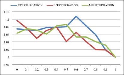
Figure 1: Approximation Ratio in Dynamic Updates

7.2 Experiments with The LETOR data set

We considered popular queries in creating a number of LETOR data sets. Each item in a LETOR data set represents a document related to a query. As such, each item $u$ has an integral relevance score $r(u)$ (relative to the query) ranging from 0 to 5, a set of feature attributes with their respective values, and a query id. Thus, we take (as ground truth), the quality score $f(S)=\sum_{u\in S}r(u)$. We define (and take as ground truth) a metric distance $f(u,v)$ function given by the cosine similarity between the feature vectors for $u$ and $v$.

For Table IV and Table V, we chose one data set (chosen at random from the original LETOR dataset) and created a data set consisting of the top (by relevance score) 50 and top 370 documents. We applied the Greedy A, Greedy B and limited local search algorithms to these two data sets for various settings of the cardinality parameter $p$. For the 50 document data set we also computed the optimal values. We observe a qualitative difference between these “real data” experiments and the experiments for synthetic data. Namely, Greedy B now has a more substantial advantage over Greedy A and corresponding decrease in the benefit of running local search for 10 times the run time of Greedy B on a given input. In contrast to the synthetic data experiments, the advantage of Greedy B over Greedy A is more pronounced for larger values of $p$, the cardinality constraint. For the $N=50$ data set and small values of $p$, the advantage stays between 3 and 4%. For the $N=370$ data set, the advantage of Greedy B over Greedy A rises to about 15% and then levels off at around 12%. The improvement due to the limited use of local search never exceeds .2% and sometimes results in no improvement. We also ran 5 different data sets (i.e. generated by 5 different queries) and averaged the results with respect to the top 50 results and all documents in each data set as shown in Table VI and Table VII. Note that in these tables, we are omitting the objective function values that have been previously included in other tables. We are averaging our results over different LETOR datasets (i.e. queries) and therefore reporting on the average objective function values wont be fully meaningful. These average results support what we found in Table IV and Table V, namely that Greedy B significantly outperforms Greedy A and that limited local search provides a very small advantage over Greedy B.

In Table VIII(e), we present the difference in the documents being returned for the 50 document data set. Here the OPT documents are the true set of optimal documents with respect to the diversification function applied to the values of the document relevance scores and the cosine distance function. As an example, consider the results for the $N=50,p=7$ setting of the parameters. Here OPT and Greedy B differ on one document while Greedy A differs on 3 documents.

7.3 Approximation Ratio in Dynamic Updates

For dynamic updates, we use same synthetic data as in Section 7.1. We have three different dynamically changing environments:

1. vperturbation: each perturbation is a weight change on an item; that is, an item (vertex) $u$ is randomly chosen and its value value is reset uniformly at random from $[0,1]$.

2. eperturbation: each perturbation is a distance change between two items; that is, a pair of distinct items $\{u,v\}$ is randmoy chosen and the distance $d(u,v)$ is reset uniformaly at random from $[1,2]$.

3. mperturbation: each perturbation is one of the above two with equal probability.

For each of the environments above and every value of $\lambda$, we start with our greedy solution (a 2-approximation) and run 20 steps of simulation, where each step consists of a random weight change of the stated type, followed by a single application of the oblivious update rule. We repeat this 100 times and record the worst approximation ratio occurring during these 100 updates. The results are shown in Fig. 1; the horizontal axis measures $\lambda$ values, and the vertical axis measures the approximation ratio.

We have the following observations:

1. In any dynamic changing environment, the maintained ratio is well below the provable ratio of 3. The worst observed ratio is about 1.11.

2. The maintained ratios are decreasing to 1 for increasing $\lambda\geq 0.6$.

From the experiment, we see that the simple local search update rule seems effective for maintaining a good approximation ratio in a dynamically changing environment.

8 Conclusion

We study the max-sum diversification with monotone submodular set functions and give a natural 2-approximation greedy algorithm for the problem when there is a cardinality constraint. We further extend the problem to matroid constraints and give a 2-approximation local search algorithm for the problem. We examine the dynamic update setting for modular set functions, where the weights and distances are constantly changing over time and the goal is to maintain a solution with good quality with a limited number of updates. We propose a simple update rule: the oblivious (single swap) update rule, and show that if the weight-perturbation is not too large, we can maintain an approximation ratio of 3 with a single update. The diversification problem has many important applications and there are many interesting future directions. Although in this paper we restricted ourselves to the max-sum objective, there are many other well-defined notion of diversity that can be considered, see for example [55] and [3]. The max-sum case can be also studied for specific metrics such as the $\ell_{1}$-norm in Euclidean space as considered by Fekete and Meijer [41] who provide a linear time optimal algorithm for constant $p$ and a PTAS when $p$ is part of the input. Their PTAS algorithm also provides a $(2+\epsilon)$-approximation for the $\ell_{2}$-norm. Their algorithms exploit the geometric nature of the metric space. Other specific metric spaces are also of interest.

In the general matroid case, the greedy algorithm given in Section 4 fails to achieve any constant approximation ratio, but one can also consider other “greedy-like algorithms” such as the partial enumeration greedy method used (for example) successfully for monotone submodular maximization subject to a knapsack constraint in Sviridenko [56]? Can such a technique also be used to provide an approximation for our diversification problem? Can our results be extended to provide a constant approximation for the diversification problem subject to a knapsack constraint? In a dynamic update setting, we only considered the oblivious single swap update rule. It is interesting to see if it is possible to maintain a better ratio than 3 with a limited number of updates, by larger cardinality swaps, and/or by a non-oblivious update rule. We leave this as an open question. The approximation ratio and application of diversification maximization in a distributed setting is pursued in a recent paper by Abbasi-Zadeh et al [1].

Finally, a crucial property used throughout our results is the triangle inequality. In our conference paper [31], we asked the question as to whether we can relate the approximation ratio to the parameter of a relaxed triangle inequality? Sydow [57] provides a partial answer to this question showing that the matching based algorithm of Hassin et al [4] can be applied to an $\alpha\geq 1$ relaxed metric (where $d(x,y)+d(y,z)\geq\alpha d(x,z))$ resulting in a (tight) $\frac{2}{\alpha}$ approximation ratio for the cardinality constrained max-sum dispersion problem. More recently and independently, Abbasi-Zadeh and Ghadiri [2] obtain the $\frac{2}{\alpha}$ approximation ratio for the cardinality constraint, and a $\frac{2}{\alpha^{2}}$ approximation ratio for an arbitrary matroid constraint.

Appendix A The Greedy Algorithm Applied to Diversification with a Matroid Constraint

We observe that for the more general matroid constraint diversification problem, the greedy algorithm in section 4 no longer achieves any constant approximation ratio. More specifically, consider the max-sum diversifciation problem as in Gallopudi and Sharma [3] (that is, for a modular quality function $f()$) but now subject to a partition matroid constraint. Partition the universe into $A=\{a,b\}$ with cardinality constraint 1 and $C=\{c_{1},c_{2},\ldots c_{r}\}$ with no cardinality constraint. Let the objective be $f(S)=\sum_{u\in S}q_{u}+\sum_{u,v\in S}d(u,v)$ where the quality and distance functions are defined as follows: $q(a)=\ell+\epsilon$, $q(x)=0$ for all $x\neq a$, and for all $x$, $d(b,x)=\ell$, $d(u,x)=\epsilon$ for all $u\neq b$. The greedy algorithm (starting with $a$ or with the best pair $(a,b)$ will yield $f(S)=f(C\cup\{a\})=\ell+\epsilon+\epsilon\cdot{r\choose 2}+r\epsilon$ while the optimal solution will be $f(C\cup\{b\})=r\cdot\ell+\epsilon\cdot{r\choose 2}$. Hence the approximation can be made arbitrarily bad by choosing $\epsilon=\frac{1}{{r\choose 2}}$ and making $r$ sufficiently large.

By the reduction in [3] to the metric dispersion problem, the above example shows that the greedy algorithm will also suffer the same unbounded approximation ratio for the metric dispersion problem.

References

- [1] S. Abbasi-Zadeh, M. Ghadiri, V. S. Mirrokni, and M. Zadimoghaddam, “Scalable feature selection via distributed diversity maximization,” To appear in AAAI 2017.
- [2] S. Abbasi-Zadeh, and M. Ghadiri, “Max-sum diversification, montone submodular functions, and semi-metric spaces,” CoRR, abs/1511.02402, 2015.
- [3] S. Gollapudi and A. Sharma, “An axiomatic approach for result diversification,” in World Wide Web Conference Series, 2009, pp. 381–390.
- [4] R. Hassin, S. Rubinstein, and A. Tamir, “Approximation algorithms for maximum dispersion,” Oper. Res. Lett., vol. 21, no. 3, pp. 133–137, 1997.
- [5] G. Nemhauser, L. Wolsey, and M. Fisher, “An analysis of the approximations for maximizing submodular set functions-i,” Mathematical Programming, vol. 14, pp. 265–294, 1978.
- [6] A. Borodin, D. Le, and Y. Ye, “Weakly submodular functions,” CoRR, vol. abs/1401.6697, 2014.
- [7] M. R. Vieira, H. L. Razente, M. C. N. Barioni, M. Hadjieleftheriou, D. Srivastava, C. T. Jr., and V. J. Tsotras, “Divdb: A system for diversifying query results,” PVLDB, vol. 4, no. 12, pp. 1395–1398, 2011.
- [8] ——, “On query result diversification,” in ICDE, 2011, pp. 1163–1174.
- [9] H. Lin and J. Bilmes, “A class of submodular functions for document summarization,” in North American chapter of the Association for Computational Linguistics/Human Language Technology Conference (NAACL/HLT-2011), Portland, OR, June 2011, (long paper).
- [10] F. Zhao, X. Zhang, A. K. H. Tung, and G. Chen, “Broad: Diversified keyword search in databases,” PVLDB, vol. 4, no. 12, pp. 1355–1358, 2011.
- [11] A. Schrijver, Combinatorial Optimization: Polyhedra and Efficiency. Springer, 2003.
- [12] J. Carbonell and J. Goldstein, “The use of mmr, diversity-based reranking for reordering documents and producing summaries,” in Proceedings of the 21st annual international ACM SIGIR conference on Research and development in information retrieval, ser. SIGIR ’98. New York, NY, USA: ACM, 1998, pp. 335–336.
- [13] D. Rafiei, K. Bharat, and A. Shukla, “Diversifying web search results,” in WWW, 2010, pp. 781–790.
- [14] N. Bansal, K. Jain, A. Kazeykina, and J. Naor, “Approximation algorithms for diversified search ranking,” in ICALP (2), 2010, pp. 273–284.
- [15] Z. Liu, P. Sun, and Y. Chen, “Structured search result differentiation,” PVLDB, vol. 2, no. 1, pp. 313–324, 2009.
- [16] C. Yu, L. Lakshmanan, and S. Amer-Yahia, “It takes variety to make a world: diversification in recommender systems,” in Proceedings of the 12th International Conference on Extending Database Technology: Advances in Database Technology, ser. EDBT ’09, 2009, pp. 368–378.
- [17] M. Drosou and E. Pitoura, “Diversity over continuous data,” IEEE Data Eng. Bull., vol. 32, no. 4, pp. 49–56, 2009.
- [18] E. Demidova, P. Fankhauser, X. Zhou, and W. Nejdl, “Divq: diversification for keyword search over structured databases,” in Proceeding of the 33rd international ACM SIGIR conference on Research and development in information retrieval, ser. SIGIR ’10. ACM, 2010, pp. 331–338.
- [19] C. Zhai, W. W. Cohen, and J. D. Lafferty, “Beyond independent relevance: methods and evaluation metrics for subtopic retrieval,” in SIGIR, 2003, pp. 10–17.
- [20] H. Chen and D. R. Karger, “Less is more: probabilistic models for retrieving fewer relevant documents,” in SIGIR, 2006, pp. 429–436.
- [21] X. Zhu, A. B. Goldberg, J. V. Gael, and D. Andrzejewski, “Improving diversity in ranking using absorbing random walks,” in HLT-NAACL, 2007, pp. 97–104.
- [22] Y. Yue and T. Joachims, “Predicting diverse subsets using structural svms,” in ICML, 2008, pp. 1224–1231.
- [23] F. Radlinski, R. Kleinberg, and T. Joachims, “Learning diverse rankings with multi-armed bandits,” in ICML, 2008, pp. 784–791.
- [24] R. Agrawal, S. Gollapudi, A. Halverson, and S. Ieong, “Diversifying search results,” in WSDM, 2009, pp. 5–14.
- [25] C. Brandt, T. Joachims, Y. Yue, and J. Bank, “Dynamic ranked retrieval,” in WSDM, 2011, pp. 247–256.
- [26] R. L. T. Santos, C. Macdonald, and I. Ounis, “Intent-aware search result diversification,” in SIGIR, 2011, pp. 595–604.
- [27] Z. Dou, S. Hu, K. Chen, R. Song, and J.-R. Wen, “Multi-dimensional search result diversification,” in WSDM, 2011, pp. 475–484.
- [28] A. Slivkins, F. Radlinski, and S. Gollapudi, “Learning optimally diverse rankings over large document collections,” in ICML, 2010, pp. 983–990.
- [29] M. Drosou and E. Pitoura, “Search result diversification,” SIGMOD Record, vol. 39, no. 1, pp. 41–47, 2010.
- [30] E. Minack, W. Siberski, and W. Nejdl, “Incremental diversification for very large sets: a streaming-based approach,” in SIGIR, 2011, pp. 585–594.
- [31] A. Borodin, H. C. Lee, and Y. Ye, “Max-sum diversification, monotone submodular functions and dynamic updates,” in PODS, 2012, pp. 155–166.
- [32] Z. Abbassi, V. S. Mirrokni, and M. Thakur, “Diversity maximization under matroid constraints,” in KDD, 2013, pp. 32–40.
- [33] E. Erkut, “The discrete p-dispersion problem,” European Journal of Operational Research, vol. 46, no. 1, pp. 48–60, May 1990. [Online]. Available: http://ideas.repec.org/a/eee/ejores/v46y1990i1p48-60.html
- [34] E. Erkut and S. Neuman, “Analytical models for locating undesirable facilities,” European Journal of Operational Research, vol. 40, no. 3, pp. 275–291, June 1989. [Online]. Available: http://ideas.repec.org/a/eee/ejores/v40y1989i3p275-291.html
- [35] M. J. Kuby, “Programming models for facility dispersion: The p-dispersion and maxisum dispersion problems,” Geographical Analysis, vol. 19, no. 4, pp. 315–329, 1987. [Online]. Available: http://dx.doi.org/10.1111/j.1538-4632.1987.tb00133.x
- [36] D. W. Wang and Y.-S. Kuo, “A study on two geometric location problems,” Inf. Process. Lett., vol. 28, pp. 281–286, August 1988.
- [37] S. S. Ravi, D. J. Rosenkrantz, and G. K. Tayi, “Heuristic and special case algorithms for dispersion problems,” Operations Research, vol. 42, no. 2, pp. 299–310, March-April 1994.
- [38] M. M. Halldórsson, K. Iwano, N. Katoh, and T. Tokuyama, “Finding subsets maximizing minimum structures,” in Symposium on Discrete Algorithms, 1995, pp. 150–159.
- [39] B. Chandra and M. M. Halldórsson, “Approximation algorithms for dispersion problems,” J. Algorithms, vol. 38, no. 2, pp. 438–465, 2001.
- [40] S. Khot, “Ruling out ptas for graph min-bisection, dense k-subgraph, and bipartite clique,” SIAM J. Comput., vol. 36, no. 4, pp. 1025–1071, 2006.
- [41] S. P. Fekete and H. Meijer, “Maximum dispersion and geometric maximum weight cliques,” Algorithmica, vol. 38, no. 3, pp. 501–511, 2003.
- [42] A. Czygrinow, “Maximum dispersion problem in dense graphs,” Oper. Res. Lett., vol. 27, no. 5, pp. 223–227, 2000.
- [43] N. Alon, “Personal communication.”
- [44] R. Meka, A. Potechin, and A. Wigderson, “Sum-of-squares lower bounds for planted clique,” in Proceedings of the Forty-Seventh Annual ACM on Symposium on Theory of Computing, STOC 2015, Portland, OR, USA, June 14-17, 2015, 2015, pp. 87–96.
- [45] N. Alon, S. Arora, R. Manoikaran, D. Moshkovitz, and O. Weinstein, “Inapproximability of densest -subgraph from aveage case harsdness,” 2011.
- [46] B. E. Birnbaum and K. J. Goldman, “An improved analysis for a greedy remote-clique algorithm using factor-revealing lps,” Algorithmica, vol. 55, no. 1, pp. 42–59, 2009.
- [47] D. Kempe, J. Kleinberg, and E. Tardos, “Maximizing the spread of influence through a social network,” in Proceedings of the ninth ACM SIGKDD international conference on Knowledge discovery and data mining, ser. KDD ’03. New York, NY, USA: ACM, 2003, pp. 137–146.
- [48] H. Lin, J. Bilmes, and S. Xie, “Graph-based submodular selection for extractive summarization,” in Proc. IEEE Automatic Speech Recognition and Understanding (ASRU), Merano, Italy, December 2009.
- [49] H. Lin and J. Bilmes, “Multi-document summarization via budgeted maximization of submodular functions,” in HLT-NAACL, 2010, pp. 912–920.
- [50] G. Călinescu, C. Chekuri, M. Pál, and J. Vondrák, “Maximizing a monotone submodular function subject to a matroid constraint,” SIAM J. Comput., vol. 40, no. 6, pp. 1740–1766, 2011.
- [51] M. Fisher, G. Nemhauser, and L. Wolsey, “An analysis of the approximations for maximizing submodular set functions-ii,” Mathematical Programming Study, vol. 8, pp. 73–87, 1978.
- [52] S. Khanna, R. Motwani, M. Sudan, and U. V. Vazirani, “On syntactic versus computational views of approximability,” Electronic Colloquium on Computational Complexity (ECCC), vol. 2, no. 23, 1995.
- [53] R. A. Brualdi, “Comments on bases in dependence structures,” Bulletin of the Australian Mathematical Society, vol. 1, no. 02, pp. 161–167, 1969.
- [54] T. Qin, T.-Y. Liu, J. Xu, and H. Li, “Letor: A benchmark collection for research on learning to rank for information retrieval,” Inf. Retr., vol. 13, no. 4, pp. 346–374, 2010.
- [55] B. Chandra and M. M. Halldórsson, “Facility dispersion and remote subgraphs,” in Proceedings of the 5th Scandinavian Workshop on Algorithm Theory. London, UK: Springer-Verlag, 1996, pp. 53–65. [Online]. Available: http://portal.acm.org/citation.cfm?id=645898.756652
- [56] M. Sviridenko, “A note on maximizing a submodular set function subject to a knapsack constraint,” Oper. Res. Lett., vol. 32, no. 1, pp. 41–43, 2004.
- [57] M. Sydow, “Improved approximation guarantee for max sum diversification with parameterised triangle inequality,” in Foundations of Intelligent Systems - 21st International Symposium, ISMIS 2014, Roskilde, Denmark, June 25-27, 2014. Proceedings, 2014, pp. 554–559.