Physics of self-sustained oscillations in the positive glow corona

Abstract

The physics of self-sustained oscillations in the phenomenon of positive glow corona is presented. The dynamics of charged-particle oscillation under static electric field has been briefly outlined; and, the resulting self-sustained current oscillations in the electrodes have been compared with the measurements from the positive glow corona experiments. The profile of self-sustained electrode current oscillations predicted by the presented theory qualitatively agrees with the experimental measurements. For instance, the experimentally observed saw-tooth shaped electrode current pulses are reproduced by the presented theory. Further, the theory correctly predicts the pulses of radiation accompanying the abrupt rises in the saw-tooth shaped current oscillations, as verified from the various glow corona experiments.

I Introduction

Consider a point particle with charge $q>0$ near the conducting sphere of radius $a$ and fixed at potential $V>0,$ which is illustrated in Fig. 1. The force acting on the charged point particle is given byJ. D. Jackson

$$\mathbf{F}=qa\left[\frac{V}{r^{3}}-\frac{q}{4\pi\epsilon_{o}\left(r^{2}-a^{2}\right)^{2}}\right]\mathbf{R},$$ (1)

where $\mathbf{R}$ is the particle’s position vector, $\epsilon_{o}$ is the vacuum permittivity, and $r$ is the radial length from sphere’s center. In Eq. (1), the force becomes negative in the limit $r$ approaches $a$ and becomes positive in the limit $r$ goes to infinity. Between these two limits, there is a point of unstable equilibrium at which the force vanishes. Such location is identified by $r=a+l_{D}$ in Fig. 1, which point represents the borderline between regions $C$ and $D.$ In region $C,$ the particle is repulsed from the sphere whereas, in region $D,$ the particle is attracted to the sphere. Why? Well, nothing surprising here. The positive point particle induces negative charges at the sphere’s surface; and, the force between the two is always attractive. This attractive force dominates in region $D,$ and the point particle is attracted to sphere there.

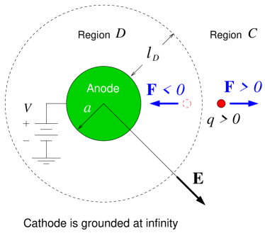
Figure 1: (Color online) Charged point particle near a conducting sphere of radius $a,$ fixed at voltage $V>0.$ In region $D,$ the particle is attracted to the sphere whereas, in region $C,$ the particle is repulsed from the sphere. The electric field, $\mathbf{E},$ is in the radially outward direction.

The same physics can be applied to describe the behavior of a charged point particle between the plane-parallel plates, which is illustrated in Fig. 2. At distances close to the anode, the charged point particle is attracted to the anode’s surface whereas, for all other distances between the plates, the particle is repulsed in the direction of the parallel plate electric field, $\mathbf{E}_{p},$ which field is present even in the absence of the charged-particle. Consequently, the space between the plates is divided into regions $C$ and $D,$ where the location of unstable equilibrium is at distance $l_{D}$ from the surface of the anode, as indicated in Fig. 2.

Figure 2: (Color online) Charged point particle inside a plane-parallel conductors separated by $h.$ In region $D,$ the particle is attracted to the anode whereas, in region $C,$ the particle is attracted to the cathode.

In both cases, the charged-particle dynamics is pretty boring. The charged point particle ends up adhering to the surface of the anode when it is in region $D$ whereas, when it is in region $C,$ the particle gets repulsed in the direction of the applied electric field. The problem becomes interesting when a charged-particle with structure is considered. Unlike the point particle, the structured particle can be polarized under externally applied electric field, such as $\mathbf{E}$ and $\mathbf{E}_{p}$ in Figs. 1 and 2, respectively. The resulting depolarization field formed inside of the structured particle redistributes the negative bound charges to the particle’s upper hemisphere surface and leaves the particle’s lower hemisphere surface depleted of the negative bound charges. Such redistribution of the bound charges inside of the structured particle is schematically illustrated in Figs. 3(a) and 3(b). As a consequence of the depolarization field inside of the structured particle, the particle is repulsed from the surface of anode in region $A$ due to the Coulomb repulsion arising between the negative charges induced at the anode’s surface and the negative bound charges formed at the surface of the particle’s upper hemisphere, as illustrated in Fig. 3(a). Such repulsive force decays rapidly outside of the region $A.$ In region $B,$ the force acting on the particle is dominated by the Coulomb attraction between the particle’s excess positive charge, $q>0,$ and the negative charges induced by it at the surface of the anode. This force is eventually overwhelmed by the Coulomb repulsion in region $A,$ and the whole process gets repeated, thereby resulting in a charged-particle oscillation in region $D.$

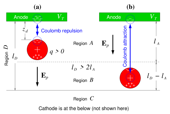
Figure 3: (Color online) (a) In case of a structured charged-particle, the region $D$ in Fig. 2 is further divided into two regions $A$ and $B.$ The particle is repulsed from the anode in region $A$ due to the Coulomb repulsion between the image charge at the anode’s surface and the negative bound charges formed at the surface of particle’s upper hemisphere. The surface of charged spherical particle is an equipotential surface; and, any excess surface charges there are uniformly distributed over it. Without confusion, the contributions from such excess charges, uniformly distributed over the surface of particle, are indicated by a big “+” symbol at the particle’s center to distinguish them from the positive bound charges associated with the induced depolarization field, which are indicated by small “+” at the particle’s lower surface. (b) The polarized charged-particle is attracted to the anode in region $B$ due to the Coulomb attraction arising between the particle’s excess charge $q$ and the image (or induced) charge associated with it at the anode’s surface. The width of region $A$ is identified by $l_{A}$ and the width of region $B$ is given by $l_{D}-l_{A},$ where $l_{D}$ is the borderline between regions $D$ and $C.$

The discussed charged-particle oscillation mechanism is intrinsic to the phenomenon of glow corona.corona-discharge-1 ; corona-discharge-2 ; corona-discharge-3 ; corona-discharge-4 ; corona-discharge-5 The self-sustained pulsing in the positive glow corona (also referred to as DC glow discharge) can be qualitatively explained from the aforementioned, oscillating, charged-particle dynamics. In this paper, I shall show that the self-sustained pulsing in the positive glow corona involves the kind of charged-particle oscillation mechanism discussed in Figs. 3(a) and 3(b). To accomplish this, I shall, first, briefly outline the dynamics of charged-particle oscillation under constant electric field. The result is then used to predict the current oscillations in the electrodes. This prediction of electrode current oscillations is compared with the results from the various glow corona experiments.

II Charged-particle oscillation in constant electric field

The dynamics of charged-particle oscillation is discussed by considering a model configuration illustrated in Fig. 4, where a core-shell structured particle has a conductive core of radius $a$ and an insulating shell of thickness $b-a.$ The conductor core has a surface free charge density of $\sigma_{1}$ and the insulator has a surface charge density of $\sigma_{2}.$ The surface charge density on the insulator has been introduced purely for mathematical generalization. In the final expression, this term can be eliminated by setting $\sigma_{2}=0\,\textnormal{C}\cdot\textnormal{m}^{-2}.$ The $\kappa_{2}$ and $\kappa_{3}$ represent the dielectric constants of the insulating shell and the space between the plates, respectively.

The potential in regions $M_{1},$ $M_{2},$ and $M_{3}$ of Fig. 4 are obtained by solving the Laplace equation, $\nabla^{2}V=0,$ with appropriate boundary conditions. Solutions $V_{1},$ $V_{2},$ and $V_{3}$ are given byCho

$$V_{1} =V_{L}+\alpha+E_{p}\left(h-s\right),\quad r\leq a,$$ (2)

$$V_{2}\left(r,\theta\right) =V_{L}+\beta+E_{p}\left(h-s+\gamma r\cos\theta\right)$$

$$-\frac{\lambda}{r}-\frac{a^{3}\gamma E_{p}\cos\theta}{r^{2}},\quad a<r\leq b,$$ (3)

$$V_{3}\left(r,\theta\right)=V_{L}+E_{p}\left(h-s+r\cos\theta\right)+\frac{\nu}{r}$$

$$\quad+\frac{\left[\gamma\left(b^{3}-a^{3}\right)-b^{3}\right]E_{p}\cos\theta}{r^{2}}+C,\quad r>b,$$ (4)

where $C$ is a constant, $\theta$ is spherical polar angle defined in Fig. 4, $r$ is radial length, $E_{p}$ is parallel-plate electric field,

$$E_{p}\equiv\left\|\mathbf{E}_{p}\right\|=\frac{V_{T}-V_{L}}{h},\quad V_{T}>V_{L};$$ (5)

and, constants $\alpha,$ $\beta,$ $\gamma,$ $\lambda,$ and $\nu$ are defined as

$$\alpha =\frac{a\left(b-a\right)\sigma_{1}}{b\epsilon_{0}\kappa_{2}}+\frac{a^{2}\sigma_{1}+b^{2}\sigma_{2}}{b\epsilon_{0}\kappa_{3}},$$

$$\beta =\frac{a\left(2b-a\right)\sigma_{1}}{b\epsilon_{0}\kappa_{2}}+\frac{a^{2}\sigma_{1}+b^{2}\sigma_{2}}{b\epsilon_{0}\kappa_{3}},$$

$$\gamma =\frac{3\kappa_{3}b^{3}}{\left(\kappa_{2}+2\kappa_{3}\right)b^{3}+2\left(\kappa_{2}-\kappa_{3}\right)a^{3}},$$ (6)

$$\lambda =\frac{a^{2}\sigma_{1}}{\epsilon_{0}\kappa_{2}},$$

$$\nu =\frac{2a\left(b-a\right)\sigma_{1}}{\epsilon_{0}\kappa_{2}}+\frac{a^{2}\sigma_{1}+b^{2}\sigma_{2}}{\epsilon_{0}\kappa_{3}}.$$

The electric displacement in region $M_{3}$ is obtained by computing

$$\mathbf{D}_{3}\left(r,\theta\right)=-\epsilon_{0}\kappa_{3}\nabla V_{3}\left(r,\theta\right),$$

where

$$\nabla=\mathbf{e}_{r}\frac{\partial}{\partial r}+\mathbf{e}_{\theta}\frac{1}{r}\frac{\partial}{\partial\theta}+\mathbf{e}_{\phi}\frac{1}{r\sin\theta}\frac{\partial}{\partial\phi},$$

$$\mathbf{e}_{r} =\mathbf{e}_{x}\sin\theta\cos\phi+\mathbf{e}_{y}\sin\theta\sin\phi+\mathbf{e}_{z}\cos\theta,$$

$$\mathbf{e}_{\theta} =\mathbf{e}_{x}\cos\theta\cos\phi+\mathbf{e}_{y}\cos\theta\sin\phi-\mathbf{e}_{z}\sin\theta,$$

$$\mathbf{e}_{\phi} =-\mathbf{e}_{x}\sin\phi+\mathbf{e}_{y}\cos\phi.$$

It can be shown that $\mathbf{e}_{z}$ component of $\mathbf{D}\left(r,\theta\right)$ in region $M_{3},$ evaluated at the anode’s surface, isCho

$$\mathbf{D}_{3;z}\left(x,y,s\right)=\mathbf{e}_{z}\epsilon_{0}\kappa_{3}\left\{\frac{3\left[\gamma\left(b^{3}-a^{3}\right)-b^{3}\right]E_{p}s^{2}}{\left(x^{2}+y^{2}+s^{2}\right)^{5/2}}\right.$$

$$\left.+\frac{\nu s-\left[\gamma\left(b^{3}-a^{3}\right)-b^{3}\right]E_{p}}{\left(x^{2}+y^{2}+s^{2}\right)^{3/2}}-E_{p}\right\}.$$

At the anode’s surface, the $\mathbf{e}_{z}$ component of $\mathbf{D}\left(x,y,z\right)$ suffers a discontinuity,

$$\mathbf{e}_{z}\cdot\mathbf{D}_{3;z}\left(x,y,s\right)=-\sigma_{iup};$$

and, the surface charge density, there, is

$$\sigma_{iup}\left(\rho,s\right) =-\epsilon_{0}\kappa_{3}\left\{\frac{3\left[\gamma\left(b^{3}-a^{3}\right)-b^{3}\right]E_{p}s^{2}}{\left(\rho^{2}+s^{2}\right)^{5/2}}\right.$$

$$\left.+\frac{\nu s-\left[\gamma\left(b^{3}-a^{3}\right)-b^{3}\right]E_{p}}{\left(\rho^{2}+s^{2}\right)^{3/2}}-E_{p}\right\},$$

where $\rho\equiv\sqrt{x^{2}+y^{2}}.$ Similarly, the $\mathbf{e}_{z}$ component of $\mathbf{D}\left(x,y,z\right)$ in region $M_{3},$ evaluated at the cathode’s surface, is

$$\mathbf{D}_{3;z}\left(x,y,s-h\right)$$

$$\quad=\mathbf{e}_{z}\epsilon_{0}\kappa_{3}\left\{\frac{3\left[\gamma\left(b^{3}-a^{3}\right)-b^{3}\right]E_{p}\left(s-h\right)^{2}}{\left[x^{2}+y^{2}+\left(s-h\right)^{2}\right]^{5/2}}\right.$$

$$\quad\left.+\frac{\nu\left(s-h\right)-\left[\gamma\left(b^{3}-a^{3}\right)-b^{3}\right]E_{p}}{\left[x^{2}+y^{2}+\left(s-h\right)^{2}\right]^{3/2}}-E_{p}\right\}.$$

At the cathode’s surface, the $\mathbf{e}_{z}$ component of $\mathbf{D}\left(x,y,z\right)$ suffers a discontinuity,

$$\mathbf{e}_{z}\cdot\mathbf{D}_{3;z}\left(x,y,s-h\right)=\sigma_{ilp};$$

and, there, the surface charge density is

$$\sigma_{ilp}\left(\rho,s\right) =\epsilon_{0}\kappa_{3}\left\{\frac{3\left[\gamma\left(b^{3}-a^{3}\right)-b^{3}\right]E_{p}\left(h-s\right)^{2}}{\left[\rho^{2}+\left(h-s\right)^{2}\right]^{5/2}}\right.$$

$$\left.-\frac{\nu\left(h-s\right)+\left[\gamma\left(b^{3}-a^{3}\right)-b^{3}\right]E_{p}}{\left[\rho^{2}+\left(h-s\right)^{2}\right]^{3/2}}-E_{p}\right\}.$$

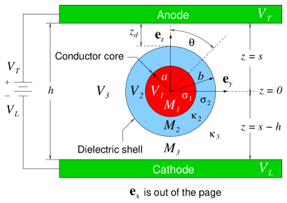
Figure 4: (Color online) Configuration showing a core-shell structured charged-particle between a DC voltage biased plane-parallel conductors.

The force acting on the particle isCho

$$\mathbf{F}_{T} =\mathbf{F}_{1}+\mathbf{F}_{2}-\mathbf{e}_{z}mg,$$ (7)

where $m$ is particle’s mass, $g=9.8\,\textnormal{m}\cdot\textnormal{s}^{-2}$ is gravitational constant; and, $\mathbf{F}_{1}$ and $\mathbf{F}_{2}$ are

$$\mathbf{F}_{1} =-\mathbf{e}_{z}\pi\nu s\int_{0}^{\rho}\frac{\sigma_{iup}\rho_{1}d\rho_{1}}{\left(\rho_{1}^{2}+s^{2}\right)^{3/2}},$$

$$\mathbf{F}_{2} =\mathbf{e}_{z}\pi\nu\left(h-s\right)\int_{0}^{\rho}\frac{\sigma_{ilp}\rho_{2}d\rho_{2}}{\left[\rho_{2}^{2}+\left(h-s\right)^{2}\right]^{3/2}}.$$

Here, $\mathbf{F}_{1}$ is the force between the charged-particle and the image charge induced by it on the surface of the anode. Similarly, $\mathbf{F}_{2}$ is the force between the charged-particle and the charge it induces at the cathode’s surface. For the parallel plate system which is microscopically large, but macroscopically small, Eq. (7) becomesCho

$$\mathbf{F}_{T}\left(s\right) =\mathbf{e}_{z}\frac{\pi\epsilon_{0}\kappa_{3}\nu}{4}\left\{\frac{\nu}{s^{2}}-\frac{\nu}{\left(h-s\right)^{2}}+\frac{\left[\gamma\left(b^{3}-a^{3}\right)-b^{3}\right]E_{p}}{s^{3}}\right.$$

$$\left.+\frac{\left[\gamma\left(b^{3}-a^{3}\right)-b^{3}\right]E_{p}}{\left(h-s\right)^{3}}-8E_{p}\right\}-\mathbf{e}_{z}mg,$$ (8)

where

$$m=\frac{4}{3}\pi\left[a^{3}\left(\rho_{m,1}-\rho_{m,2}\right)+b^{3}\rho_{m,2}\right]$$

with $\rho_{m,1}$ and $\rho_{m,2}$ representing mass densities of the particle’s core and shell, respectively.

The force $\mathbf{F}_{T}\left(s\right)$ of Eq. (8) is plotted using the following parameter values:

$$\left\{\begin{array}[]{c}\kappa_{2}=6,\quad\kappa_{3}=1,\\ a=1.5\,\mu\textnormal{m},\quad h=1\,\textnormal{mm},\\ b-a=4\,\textnormal{nm},\\ V_{L}=0\,\textnormal{V},\\ \sigma_{2}=0\,\textnormal{C}\cdot\textnormal{m}^{-2}\textnormal{ (i.e., insulator)},\\ \rho_{m,1}=2700\,\textnormal{kg}\cdot\textnormal{m}^{-3},\\ \rho_{m,2}=3800\,\textnormal{kg}\cdot\textnormal{m}^{-3},\end{array}\right.$$ (9)

where the choice of $4\,\textnormal{nm}$ for the shell’s thickness and a dielectric constant of $k_{2}\sim 6$ are typical for alumina nanoparticles.Japan-al2o3 ; al203 To compare the cases which involve the positively and the negatively charged particles, the surface charge densities of $\sigma_{1}=0.012\,\textnormal{C}\cdot\textnormal{m}^{-2}$ and $\sigma_{1}=-0.012\,\textnormal{C}\cdot\textnormal{m}^{-2}$ have been considered. For the force dependence on the applied parallel plate electric fields, $V_{T}=0\,\textnormal{V}$ and $V_{T}=500\,\textnormal{V}$ have been considered for comparison. The $V_{T}=0\,\textnormal{V}$ corresponds to the case where a charged-particle is placed between the grounded plane-parallel plates. With $V_{L}=0\,\textnormal{V}$ and $h=1\,\textnormal{mm},$ the anode voltage of $V_{T}=500\,\textnormal{V}$ corresponds to the parallel plate electric field of $E_{p}=500\,\textnormal{kV}\cdot\textnormal{m}^{-1}.$ The results are shown in Fig. 5(a). As expected, when both plates are grounded, the charged-particle is attracted to the nearest grounded plate. For instance, in the region where $s<0.5\,\textnormal{mm},$ the force $\mathbf{F}_{T}\left(s\right)$ is positive whereas, for $s>0.5\,\textnormal{mm},$ the force becomes negative. Right at the midway between the plates, i.e., $s=h/2,$ the net force on the charged-particle vanishes. Why? This is because, at $s=h/2,$ the particle is equal distance away from the surfaces of the anode and the cathode plates; and, in such situation, the charges of opposite polarity are induced at the surfaces of the anode and the cathode with equal magnitudes. Finally, the presence of the parallel plate electric field, $\left\|\mathbf{E}_{p}\right\|>0,$ offsets the force to the negative axis for positively charged particles. The resulting offset in the force gives rise to the oscillatory behavior of the positively charged particle in vicinity of the anode.

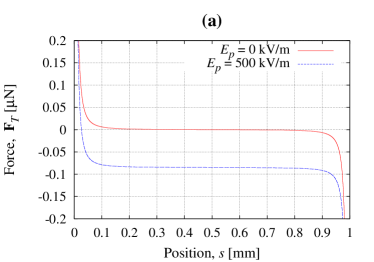
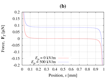
Figure 5: (Color online) Plot of $\mathbf{F}_{T}\left(s\right),$ Eq. (8), for $E_{p}=0\,\textnormal{kV}\cdot\textnormal{m}^{-1}$ and $E_{p}=500\,\textnormal{kV}\cdot\textnormal{m}^{-1}.$ (a) The case of a positively charged particle, where $\sigma_{1}=0.012\,\textnormal{C}\cdot\textnormal{m}^{-2}.$ (b) The case of a negatively charged particle, where $\sigma_{1}=-0.012\,\textnormal{C}\cdot\textnormal{m}^{-2}.$ In both (a) and (b), all other parameter values are as defined in Eq. (9). The anode is located at the left side.

What happens to the force, $\mathbf{F}_{T}\left(s\right),$ when the particle is negatively charged? Equation (8) has been plotted using the same parameter values defined in Eq. (9) with the charge density of $\sigma_{1}=-0.012\,\textnormal{C}\cdot\textnormal{m}^{-2}$ for a negatively charged particle. The results are shown in Fig. 5(b), where $E_{p}=0\,\textnormal{kV}\cdot\textnormal{m}^{-1}$ and $E_{p}=500\,\textnormal{kV}\cdot\textnormal{m}^{-1}$ have been considered for comparison. As with the case of positively charge particle, the negatively charged particle is attracted to the closest electrode when $E_{p}=0\,\textnormal{kV}\cdot\textnormal{m}^{-1}.$ At the midway between the plates, i.e., $s=h/2,$ the negatively charged particle feels no net force due to the fact that charges of opposite polarity are induced at the facing surfaces of each plates with equal magnitude. At the presence of the parallel plate electric field, i.e., $E_{p}=500\,\textnormal{kV}\cdot\textnormal{m}^{-1}$ in Fig. 5(b), the force offsets to the positive axis. The resulting offset in the force gives rise to the oscillatory behavior of the negatively charged particle in vicinity of the cathode.

The physical charged-particle with structure cannot penetrate into the surfaces of the anode and the cathode plates, of course. Therefore, the parameter $s$ in Figs. 5(a) and 5(b) are restricted to a domain $b\leq s\leq h-b,$ where $b$ is the charged-particle’s radius and $h$ is the gap between the anode and the cathode plates. The case of $s=b$ corresponds to the situation where the particle is in contact with the anode’s surface; and, the case of $s=h-b$ corresponds to the situation where the particle is in contact with the surface of the cathode. For this reason, the magnitude of the force acting on the charged-particle remains finite at $s=b$ and $s=h-b$ in Figs. 5(a) and 5(b).

II.1 Positively charged particle with structure

II.1.1 Constituent forces

It is worthwhile to discuss the constituent forces of $\mathbf{F}_{T}.$ When particle is sufficiently charged, the gravitational force becomes negligible; and, Eq. (8) can be expressed as

$$\mathbf{F}_{T}=\underbrace{\mathbf{f}_{1,1}+\mathbf{f}_{1,2}+\mathbf{f}_{1,3}}_{\mathbf{F}_{1}}+\underbrace{\mathbf{f}_{2,1}+\mathbf{f}_{2,2}+\mathbf{f}_{2,3}}_{\mathbf{F}_{2}},$$

where the constituent forces of $\mathbf{F}_{1}$ are

$$\mathbf{f}_{1,1} =\mathbf{e}_{z}\frac{\pi\epsilon_{0}\kappa_{3}\nu^{2}}{4s^{2}},$$

$$\mathbf{f}_{1,2} =\mathbf{e}_{z}\frac{\pi\epsilon_{0}\kappa_{3}\nu\left[\gamma\left(b^{3}-a^{3}\right)-b^{3}\right]E_{p}}{4s^{3}},$$

$$\mathbf{f}_{1,3} =-\mathbf{e}_{z}\pi\epsilon_{0}\kappa_{3}\nu E_{p};$$

and for $\mathbf{F}_{2},$ its constituent forces take on the form given by

$$\mathbf{f}_{2,1} =-\mathbf{e}_{z}\frac{\pi\epsilon_{0}\kappa_{3}\nu^{2}}{4\left(h-s\right)^{2}},$$

$$\mathbf{f}_{2,2} =\mathbf{e}_{z}\frac{\pi\epsilon_{0}\kappa_{3}\nu\left[\gamma\left(b^{3}-a^{3}\right)-b^{3}\right]E_{p}}{4\left(h-s\right)^{3}},$$

$$\mathbf{f}_{2,3} =-\mathbf{e}_{z}\pi\epsilon_{0}\kappa_{3}\nu E_{p}.$$

Since $\nu>0$ and $1>\gamma>0,$ one finds

$$\gamma\left(b^{3}-a^{3}\right)-b^{3}<0;$$

and, the previous constituent force terms of $\mathbf{F}_{1}$ behave as

$$\mathbf{f}_{1,1}\sim\mathbf{e}_{z}\frac{1}{s^{2}},\quad\mathbf{f}_{1,2}\sim-\mathbf{e}_{z}\frac{E_{p}}{s^{3}},\quad\mathbf{f}_{1,3}\sim-\mathbf{e}_{z}E_{p};$$

whereas for $\mathbf{F}_{2},$

$$\mathbf{f}_{2,1}\sim-\mathbf{e}_{z}\frac{1}{\left(h-s\right)^{2}},\quad\mathbf{f}_{2,2}\sim-\mathbf{e}_{z}\frac{E_{p}}{\left(h-s\right)^{3}},\quad\mathbf{f}_{2,3}\sim-\mathbf{e}_{z}E_{p}.$$

Physically, $\mathbf{f}_{1,1}$ ($\mathbf{f}_{2,1}$) represents an attractive force between charged particle and its image charge at the surface of anode (cathode). The $\mathbf{f}_{1,3}$ ($\mathbf{f}_{2,3}$) represents the usual force on charged-particle by parallel plate electric field, $\mathbf{E}_{p}.$ The other force term, $\mathbf{f}_{1,2}$ ($\mathbf{f}_{2,2}$), arises as a consequence of a structured particle that becomes polarized under $\mathbf{E}_{p}.$ Such force vanishes in the absence $\mathbf{E}_{p}.$

So, what gives rise to charged-particle oscillation? The $\mathbf{F}_{2}$ cannot generate oscillations because $\mathbf{f}_{2,1},$ $\mathbf{f}_{2,2},$ and $\mathbf{f}_{2,3}$ are all directed in the same direction. The $\mathbf{F}_{1},$ on the other hand, contains constituent forces with opposite directions that compete one another; and, such terms generate oscillations. For instance, at distances very close to the anode, $\mathbf{F}_{1}\approx\mathbf{f}_{1,2}\sim-\mathbf{e}_{z}E_{p}s^{-3};$ and, such force is responsible for the Coulomb repulsion in region $A$ of Fig. 3(a). This force decays rapidly with distance. Consequently, outside of the region $A,$ the contributions from $\mathbf{f}_{1,2}$ become negligible. In region $B,$ e.g., Fig. 3(b), the force on the particle is dominated by $\mathbf{F}_{1}\approx\mathbf{f}_{1,1}\sim\mathbf{e}_{z}s^{-2}.$ This force attracts the charged-particle back to the anode. It is this “push-pull” competition between $\mathbf{f}_{1,1}$ and $\mathbf{f}_{1,2}$ that gives rise to charged-particle oscillation in region $D,$ as illustrated in Fig. 6.

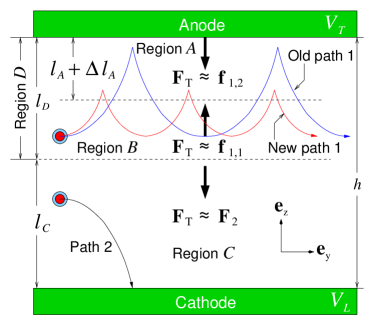
Figure 6: (Color online) Schematic illustration of positively charged, structured, particle oscillating in vicinity of the anode. The dominant constituent force terms are shown in regions $A$ and $B.$ No oscillation mode exists near the cathode, region $C,$ for a positive particle. The old path 1, new path 1, and the path 2 represent the schematic plot of $z_{d}\left(t\right)$ versus time, where time is the horizontal axis. The new path 1 corresponds to a case where $E_{p}$ is higher than the one in old path 1.

The width $l_{A}$ of region $A$ increases with $E_{p}$ as a consequence of $\mathbf{f}_{1,2}\sim-\mathbf{e}_{z}E_{p}s^{-3}.$ If region $A$ widens by $\Delta l_{A},$ the width of region $B$ decreases by the same amount. This is because the width $l_{D}$ of region $D$ remains fixed for a given charged-particle of constant excess charge $q.$ Consequently, the particle’s oscillation frequency increases with $E_{p}$ in region $D.$ Such is schematically illustrated in Fig. 6. The $\textnormal{new path 1},$ which is the plot of $z_{d}\left(t\right)$ versus time corresponding to the case of higher $E_{p},$ has a higher oscillation frequency than the $\textnormal{old path 1}.$

II.1.2 Potential energy

By definition, the force $\mathbf{F}$ is defined as the negative gradient of the potential energy function $U,$

$$\mathbf{F}\equiv-\nabla U.$$

For a one dimensional force, such as the one in Eq. (8), this implies

$$\mathbf{F}_{T}\left(s\right)=-\mathbf{e}_{z}\frac{dU}{ds},$$

where $U\equiv U\left(s\right).$ The one dimensional potential energy function, $U\left(s\right),$ becomes

$$U\left(s\right)=-\int_{s_{\textnormal{ref}}}^{s}\mathbf{F}_{T}\cdot\mathbf{e}_{z}ds,$$ (10)

where $s_{\textnormal{ref}}$ is the reference point in which $U\left(s_{\textnormal{ref}}\right)<U\left(s\right).$ For instance, at the presence of the parallel plate electric field, $\mathbf{E}_{p},$ the potential energy of a positively charged particle may be computed by integrating the line integral along the path illustrated in Fig. 7(a). On the other hand, the potential energy for a negatively charged particle subjected to the same parallel plate electric field can be computed by integrating the line integral along the path illustrated in Fig. 7(b). Consequently, the presence of electric field, $\mathbf{E}_{p},$ as well as its directions and the polarity of the charged-particle affect the choice of $s_{\textnormal{ref}}$ in the line integral of Eq. (10). For such reason, I shall only consider the case where $\left\|\mathbf{E}_{p}\right\|>0$ for the evaluation of $U\left(s\right).$

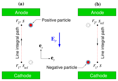
Figure 7: (Color online) Illustrates the integral path in a line integral for a given parallel plate electric field $\mathbf{E}_{p}.$ (a) The case of positively charged particle. (b) The case of negatively charged particle.

That said, Eq. (8) is inserted for $\mathbf{F}_{T}$ in Eq. (10) to yield

$$U\left(s\right) =-\frac{\pi\epsilon_{0}\kappa_{3}\nu}{4}\int_{s_{\textnormal{ref}}}^{s}\left\{\frac{\nu}{s^{2}}-\frac{\nu}{\left(h-s\right)^{2}}\right.$$

$$+\frac{\left[\gamma\left(b^{3}-a^{3}\right)-b^{3}\right]E_{p}}{s^{3}}$$

$$\left.+\frac{\left[\gamma\left(b^{3}-a^{3}\right)-b^{3}\right]E_{p}}{\left(h-s\right)^{3}}-8E_{p}\right\}ds$$

$$+mg\int_{s_{\textnormal{ref}}}^{s}ds,$$ (11)

where $E_{p}>0.$ Equation (11) is evaluated utilizing the following integral formulas:

$$\int_{s_{\textnormal{ref}}}^{s}ds =s-s_{\textnormal{ref}},$$

$$\int_{s_{\textnormal{ref}}}^{s}\frac{1}{s^{2}}ds =\frac{1}{s_{\textnormal{ref}}}-\frac{1}{s},$$

$$\int_{s_{\textnormal{ref}}}^{s}\frac{1}{s^{3}}ds =\frac{1}{2s_{\textnormal{ref}}^{2}}-\frac{1}{2s^{2}},$$

$$\int_{s_{\textnormal{ref}}}^{s}\frac{1}{\left(h-s\right)^{2}}ds =\frac{1}{h-s}-\frac{1}{h-s_{\textnormal{ref}}},$$

$$\int_{s_{\textnormal{ref}}}^{s}\frac{1}{\left(h-s\right)^{3}}ds =\frac{1}{2\left(h-s\right)^{2}}-\frac{1}{2\left(h-s_{\textnormal{ref}}\right)^{2}}.$$

The result is

$$U\left(s\right) =\frac{\pi\epsilon_{0}\kappa_{3}\nu}{4}\left\{\frac{\nu}{s}+\frac{\nu}{h-s}+\frac{\left[\gamma\left(b^{3}-a^{3}\right)-b^{3}\right]E_{p}}{2s^{2}}\right.$$

$$\left.-\frac{\left[\gamma\left(b^{3}-a^{3}\right)-b^{3}\right]E_{p}}{2\left(h-s\right)^{2}}+8E_{p}s\right\}+mgs$$

$$-\frac{\pi\epsilon_{0}\kappa_{3}\nu}{4}\left\{\frac{\nu}{s_{\textnormal{ref}}}+\frac{\nu}{h-s_{\textnormal{ref}}}+\frac{\left[\gamma\left(b^{3}-a^{3}\right)-b^{3}\right]E_{p}}{2s_{\textnormal{ref}}^{2}}\right.$$

$$\left.-\frac{\left[\gamma\left(b^{3}-a^{3}\right)-b^{3}\right]E_{p}}{2\left(h-s_{\textnormal{ref}}\right)^{2}}+8E_{p}s_{\textnormal{ref}}\right\}-mgs_{\textnormal{ref}},$$ (12)

where $E_{p}>0.$ The parameter $s$ is related to the parameter $z_{d},$ which is defined in Fig. 4, by

$$s=z_{d}+b\quad\textnormal{and}\quad\ddot{s}=\ddot{z}_{d}.$$ (13)

Utilizing this definition, Eq. (12) can be rewritten as

$$U\left(z_{d}\right) =\frac{\pi\epsilon_{0}\kappa_{3}\nu}{4}\left\{\frac{\nu}{z_{d}+b}+\frac{\nu}{h-z_{d}-b}\right.$$

$$+\frac{\left[\gamma\left(b^{3}-a^{3}\right)-b^{3}\right]E_{p}}{2\left(z_{d}+b\right)^{2}}-\frac{\left[\gamma\left(b^{3}-a^{3}\right)-b^{3}\right]E_{p}}{2\left(h-z_{d}-b\right)^{2}}$$

$$\left.+8E_{p}\left(z_{d}+b\right)\vphantom{\frac{\nu}{z_{d}+b}}\right\}+mg\left(z_{d}+b\right)$$

$$-\frac{\pi\epsilon_{0}\kappa_{3}\nu}{4}\left\{\frac{\nu}{s_{\textnormal{ref}}}+\frac{\nu}{h-s_{\textnormal{ref}}}+\frac{\left[\gamma\left(b^{3}-a^{3}\right)-b^{3}\right]E_{p}}{2s_{\textnormal{ref}}^{2}}\right.$$

$$\left.-\frac{\left[\gamma\left(b^{3}-a^{3}\right)-b^{3}\right]E_{p}}{2\left(h-s_{\textnormal{ref}}\right)^{2}}+8E_{p}s_{0}\right\}-mgs_{\textnormal{ref}},$$

where $E_{p}>0.$ I shall set $s_{\textnormal{ref}}$ at the midway between the parallel plates,

$$s_{\textnormal{ref}}=\frac{h}{2};$$ (14)

and the $U\left(z_{d}\right)$ becomes

$$U\left(z_{d}\right) =\frac{\pi\epsilon_{0}\kappa_{3}\nu}{4}\left\{\frac{\nu}{z_{d}+b}+\frac{\nu}{h-z_{d}-b}\right.$$

$$+\frac{\left[\gamma\left(b^{3}-a^{3}\right)-b^{3}\right]E_{p}}{2\left(z_{d}+b\right)^{2}}-\frac{\left[\gamma\left(b^{3}-a^{3}\right)-b^{3}\right]E_{p}}{2\left(h-z_{d}-b\right)^{2}}$$

$$\left.+8E_{p}\left(z_{d}+b\right)\vphantom{\frac{\nu}{z_{d}+b}}\right\}+mg\left(z_{d}+b\right)$$

$$-\frac{\pi\epsilon_{0}\kappa_{3}\nu}{h}\left(\nu+E_{p}h^{2}\right)-\frac{1}{2}mgh,$$ (15)

where $E_{p}>0;$ and, the explicit expressions for $E_{p},$ $\gamma,$ and $\nu$ are defined in Eqs. (5) and (6):

$$E_{p} =\frac{V_{T}-V_{L}}{h},\quad V_{T}>V_{L};$$

$$\gamma =\frac{3\kappa_{3}b^{3}}{\left(\kappa_{2}+2\kappa_{3}\right)b^{3}+2\left(\kappa_{2}-\kappa_{3}\right)a^{3}},$$

$$\nu =\frac{2a\left(b-a\right)\sigma_{1}}{\epsilon_{0}\kappa_{2}}+\frac{a^{2}\sigma_{1}+b^{2}\sigma_{2}}{\epsilon_{0}\kappa_{3}}.$$

Equation (15) is plotted for a positively charged particle in which $\sigma_{1}=0.012\,\textnormal{C}\cdot\textnormal{m}^{-2}$ and all other parameter values are same as defined in Eq. (9),

$$\left\{\begin{array}[]{c}\kappa_{2}=6,\quad\kappa_{3}=1,\\ a=1.5\,\mu\textnormal{m},\quad h=1\,\textnormal{mm},\\ b-a=4\,\textnormal{nm},\\ V_{L}=0\,\textnormal{V},\\ \sigma_{2}=0\,\textnormal{C}\cdot\textnormal{m}^{-2}\textnormal{ (i.e., insulator)},\\ \rho_{m,1}=2700\,\textnormal{kg}\cdot\textnormal{m}^{-3},\\ \rho_{m,2}=3800\,\textnormal{kg}\cdot\textnormal{m}^{-3}.\end{array}\right.$$

For the plot, the anode voltages of $V_{T}=1\,\textnormal{kV},$ $V_{T}=2\,\textnormal{kV},$ and $V_{T}=3\,\textnormal{kV}$ are considered for comparison. For $V_{L}=0\,\textnormal{V}$ and $h=1\,\textnormal{mm},$ these anode voltages correspond to the parallel plate electric field strengths of $E_{p}=1\,\textnormal{MV}\cdot\textnormal{m}^{-1},$ $E_{p}=2\,\textnormal{MV}\cdot\textnormal{m}^{-1},$ and $E_{p}=3\,\textnormal{MV}\cdot\textnormal{m}^{-1},$ respectively. The results are shown in Figs. 8(a) and 8(b), where the “potential well” corresponding to each $E_{p}$ are formed near the anode. The depth of the “potential well,” wherein the charged-particle can have oscillatory solutions, depends on the magnitude of the applied parallel plate electric field. Because the physical particle cannot penetrate into the surface of the anode, the parameter $z_{d}$ cannot be negative valued. When $z_{d}=0\,\mu\textnormal{m},$ the particle is right on the anode’s surface; and, this restricts the height of the potential well at $z_{d}=0\,\mu\textnormal{m}$ to a finite value, which can be verified from Fig. 8(b). In the case of $E_{p}=1\,\textnormal{MV}\cdot\textnormal{m}^{-1},$ the width of the potential well is approximately $\sim 250\,\mu\textnormal{m}$ and the particle is restricted to $0\,\mu\textnormal{m}<z_{d}\lesssim 250\,\mu\textnormal{m}$ for oscillations. The width of the potential well decreases with the applied parallel plate electric field. For instance, in the case of $E_{p}=2\,\textnormal{MV}\cdot\textnormal{m}^{-1},$ the potential well width is approximately $\sim 125\,\mu\textnormal{m}$ and the particle is restricted to $0\,\mu\textnormal{m}<z_{d}\lesssim 125\,\mu\textnormal{m}$ for oscillations. Physically, this corresponds to the narrowing of the positive glow region with increased $E_{p}.$

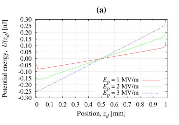
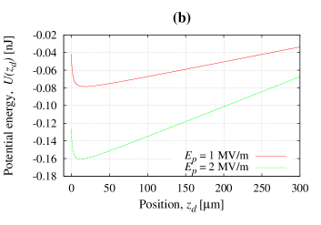
Figure 8: (Color online) (a) Plot of the potential energy function, $U\left(z_{d}\right)$ of Eq. (15), for $E_{p}=1\,\textnormal{MV}\cdot\textnormal{m}^{-1},$ $E_{p}=2\,\textnormal{MV}\cdot\textnormal{m}^{-1},$ and $E_{p}=3\,\textnormal{MV}\cdot\textnormal{m}^{-1}.$ The particle has a charge density of $\sigma_{1}=0.012\,\textnormal{C}\cdot\textnormal{m}^{-2}$ and all other parameter values are as defined in Eq. (9). (b) Enlarged plot of $U\left(z_{d}\right)$ for domain $0<z_{d}<h/2,$ where $h=1\,\textnormal{mm}.$ In the plot, the anode is located at $z_{d}=0\,\mu\textnormal{m}.$

II.1.3 Dynamics in nonrelativistic regime

The particle’s equation of motion, in the nonrelativistic limit, is obtained by solving

$$\mathbf{e}_{z}m\ddot{s}=\mathbf{F}_{T},$$ (16)

where $\ddot{s}\equiv d^{2}s/dt^{2}$ is the particle’s acceleration. Insertion of Eq. (8) for $\mathbf{F}_{T}$ in Eq. (16) yields

$$\ddot{s} =\frac{\pi\epsilon_{0}\kappa_{3}\nu}{4m}\left\{\frac{\nu}{s^{2}}-\frac{\nu}{\left(h-s\right)^{2}}+\frac{\left[\gamma\left(b^{3}-a^{3}\right)-b^{3}\right]E_{p}}{s^{3}}\right.$$

$$\left.+\frac{\left[\gamma\left(b^{3}-a^{3}\right)-b^{3}\right]E_{p}}{\left(h-s\right)^{3}}-8E_{p}\right\}-g,$$

where $\mathbf{e}_{z}$ has been dropped for convenience. Utilizing the relations in Eq. (13), this can be rewritten as

$$\ddot{z}_{d} =\frac{\pi\epsilon_{0}\kappa_{3}\nu}{4m}\left\{\frac{\nu}{\left(z_{d}+b\right)^{2}}-\frac{\nu}{\left(h-z_{d}-b\right)^{2}}\right.$$

$$+\frac{\left[\gamma\left(b^{3}-a^{3}\right)-b^{3}\right]E_{p}}{\left(z_{d}+b\right)^{3}}$$

$$\left.+\frac{\left[\gamma\left(b^{3}-a^{3}\right)-b^{3}\right]E_{p}}{\left(h-z_{d}-b\right)^{3}}-8E_{p}\right\}-g.$$ (17)

Equation (17) is solved via Runge-Kutta method. For the parameter values, I shall use the same values specified in Eq. (9) with $\sigma_{1}=0.012\,\textnormal{C}\cdot\textnormal{m}^{-2}.$ For the initial conditions, I shall choose

$$z_{d}\left(0\right)=30\,\mu\textnormal{m}\quad\textnormal{and}\quad\dot{z}_{d}\left(0\right)=0.$$ (18)

The initial condition for the particle’s position has been chosen from the consideration of the potential energy function illustrated in Fig. 8; for instance, $z_{d}\left(0\right)=30\,\mu\textnormal{m}$ is within the potential well illustrated in Fig. 8(b). The anode voltages of $V_{T}=1\,\textnormal{kV}$ and $V_{T}=2\,\textnormal{kV}$ have been considered for comparison. For $V_{L}=0\,\textnormal{V}$ and $h=1\,\textnormal{mm},$ the anode voltages of $V_{T}=1\,\textnormal{kV}$ and $V_{T}=2\,\textnormal{kV}$ corresponds to parallel plate electric field strengths of $E_{p}=1\,\textnormal{MV}\cdot\textnormal{m}^{-1}$ and $E_{p}=2\,\textnormal{MV}\cdot\textnormal{m}^{-1},$ respectively. The results are shown in Fig. 9. The dependence of oscillation frequency on $E_{p}$ is consistent with the argument discussed previously in Fig. 6.

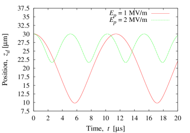
Figure 9: (Color online) Oscillating positively charged nonrelativistic particle with structure in vicinity of the anode. The plot of $z_{d}\left(t\right)$ has been obtained from Eq. (17) using the initial conditions specified in Eq. (18) and the parameter values specified in Eq. (9) with $\sigma_{1}=0.012\,\textnormal{C}\cdot\textnormal{m}^{-2}.$ In the plot, the anode is located at $z_{d}=0\,\mu\textnormal{m}.$

II.1.4 Dynamics in relativistic regime

In the relativistic generalization, the equation of motion for the charged-particle is obtained by solving

$$\mathbf{e}_{z}\frac{d}{dt}\left[\frac{m\dot{s}}{\sqrt{1-\left(\frac{\dot{s}}{c}\right)^{2}}}\right]=\mathbf{F}_{T},$$ (19)

where $c=3\times 10^{8}\,\textnormal{m}\cdot\textnormal{s}^{-1}$ is the speed of light in vacuum and $\dot{s}=ds/dt$ is the charged-particle’s speed. Insertion of Eq. (8) for $\mathbf{F}_{T}$ in Eq. (19), and after some rearrangements, yieldsCho

$$\ddot{s} =\left(1-\frac{\dot{s}^{2}}{c^{2}}\right)^{3/2}\left(\frac{\pi\epsilon_{0}\kappa_{3}\nu}{4m}\left\{\frac{\nu}{s^{2}}-\frac{\nu}{\left(h-s\right)^{2}}\right.\right.$$

$$+\frac{\left[\gamma\left(b^{3}-a^{3}\right)-b^{3}\right]E_{p}}{s^{3}}$$

$$\left.\left.+\frac{\left[\gamma\left(b^{3}-a^{3}\right)-b^{3}\right]E_{p}}{\left(h-s\right)^{3}}-8E_{p}\right\}-g\right),$$ (20)

where $\mathbf{e}_{z}$ has been dropped for convenience. The $z_{d}$ parameter defined in Fig. 4 is related to the parameter $s$ by

$$s=z_{d}+b,\quad\dot{s}=\dot{z}_{d},\quad\ddot{s}=\ddot{z}_{d};$$

and the expression in Eq. (20) becomes

$$\ddot{z}_{d} =\left(1-\frac{\dot{z}_{d}^{2}}{c^{2}}\right)^{3/2}\left(\frac{\pi\epsilon_{0}\kappa_{3}\nu}{4m}\left\{\frac{\nu}{\left(z_{d}+b\right)^{2}}\right.\right.$$

$$-\frac{\nu}{\left(h-z_{d}-b\right)^{2}}+\frac{\left[\gamma\left(b^{3}-a^{3}\right)-b^{3}\right]E_{p}}{\left(z_{d}+b\right)^{3}}$$

$$\left.\left.+\frac{\left[\gamma\left(b^{3}-a^{3}\right)-b^{3}\right]E_{p}}{\left(h-z_{d}-b\right)^{3}}-8E_{p}\right\}-g\right).$$ (21)

Equation (21) describes the charged-particle’s motion at all speed ranges.

II.2 Negatively charged particle with structure

II.2.1 Constituent forces

For negatively charged core-shell structured particle, neglecting the gravity, $\mathbf{F}_{T}$ of Eq. (8) gets modified asCho

$$\mathbf{F}_{T}=\underbrace{\mathbf{n}_{1,1}+\mathbf{n}_{1,2}+\mathbf{n}_{1,3}}_{\mathbf{N}_{1}}+\underbrace{\mathbf{n}_{2,1}+\mathbf{n}_{2,2}+\mathbf{n}_{2,3}}_{\mathbf{N}_{2}},$$

where the constituent forces of $\mathbf{N}_{1}$ are

$$\mathbf{n}_{1,1} =\mathbf{e}_{z}\frac{\pi\epsilon_{0}\kappa_{3}\nu^{2}}{4s^{2}}\sim\mathbf{e}_{z}\frac{1}{s^{2}},$$

$$\mathbf{n}_{1,2} =\mathbf{e}_{z}\frac{\pi\epsilon_{0}\kappa_{3}\left|\nu\right|\left|\gamma\left(b^{3}-a^{3}\right)-b^{3}\right|E_{p}}{4s^{3}}\sim\mathbf{e}_{z}\frac{E_{p}}{s^{3}},$$

$$\mathbf{n}_{1,3} =\mathbf{e}_{z}\pi\epsilon_{0}\kappa_{3}\left|\nu\right|E_{p}\sim\mathbf{e}_{z}E_{p};$$

and the constituent forces of $\mathbf{N}_{2}$ are given by

$$\mathbf{n}_{2,1} =-\mathbf{e}_{z}\frac{\pi\epsilon_{0}\kappa_{3}\nu^{2}}{4\left(h-s\right)^{2}}\sim-\mathbf{e}_{z}\frac{1}{\left(h-s\right)^{2}},$$

$$\mathbf{n}_{2,2} =\mathbf{e}_{z}\frac{\pi\epsilon_{0}\kappa_{3}\left|\nu\right|\left|\gamma\left(b^{3}-a^{3}\right)-b^{3}\right|E_{p}}{4\left(h-s\right)^{3}}\sim\mathbf{e}_{z}\frac{E_{p}}{\left(h-s\right)^{3}},$$

$$\mathbf{n}_{2,3} =\mathbf{e}_{z}\pi\epsilon_{0}\kappa_{3}\left|\nu\right|E_{p}\sim\mathbf{e}_{z}E_{p}.$$

Here, $\mathbf{N}_{1}$ is the force between charged-particle and its image charge formed at the anode’s surface whereas $\mathbf{N}_{2}$ corresponds to the force between charged-particle and its image charge contribution at the cathode’s surface. The notations $\left(\mathbf{N}_{1},\mathbf{N}_{2}\right)$ are introduced to distinguish from $\left(\mathbf{F}_{1},\mathbf{F}_{2}\right)$ of the positive charged-particle case. In the case of negative charged-particle, the force $\mathbf{N}_{2}$ gives rise to oscillations; and, the particle oscillates in vicinity of the cathode, as schematically illustrated in Fig. 10.

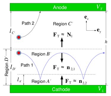
Figure 10: (Color online) Illustration of negatively charged, structured, particle oscillating in vicinity of the cathode, i.e., the regions $A^{\prime}$ and $B^{\prime}.$ The dominant constituent force terms are shown in regions $A^{\prime}$ and $B^{\prime}.$ No oscillation mode exists near the anode, i.e., the region $C^{\prime}.$ The width of the region $A^{\prime}$ is identified by $l_{A^{\prime}},$ and the width of the region $B^{\prime}$ is given by $l_{D^{\prime}}-l_{A^{\prime}},$ where $l_{D^{\prime}}$ is the borderline between the regions $B^{\prime}$ and $C^{\prime}.$ The path 1 and path 2 represent the schematic plot of $z_{d}\left(t\right)$ versus time, where the horizontal axis is the time.

To validate the argument illustrated in Fig. 10, Eq. (17) is evaluated for a negatively charged particle, $\sigma_{1}=-0.012\,\textnormal{C}\cdot\textnormal{m}^{-2},$ using the following initial conditions:

$$z_{d}\left(0\right)=h-2b-z_{d}^{\prime}\quad\textnormal{and}\quad\dot{z}_{d}\left(0\right)=0,$$ (22)

where $z_{d}^{\prime}=30\,\mu\textnormal{m}.$ To compare the result against the positively charged particle situation discussed in Fig. 9, the particle’s initial position has been assigned such that there is a gap of $30\,\mu\textnormal{m}$ between the particle’s lower surface and the cathode’s surface. The choice of $z_{d}^{\prime}=30\,\mu\textnormal{m}$ in Eq. (22) ensures such criteria. The parallel plate electric field strength of $E_{p}=2\,\textnormal{MV}\cdot\textnormal{m}^{-1}$ is chosen. For all other parameter values, the same values from Eq. (9) are used. That said, the result is plotted in Fig. 11, where it shows the oscillation frequency and the oscillation amplitude identical to the positively charged particle case corresponding to $E_{p}=2\,\textnormal{MV}\cdot\textnormal{m}^{-1}$ in Fig. 9. This time, however, the charged-particle oscillates near the cathode instead of the anode, as it is negatively charged.

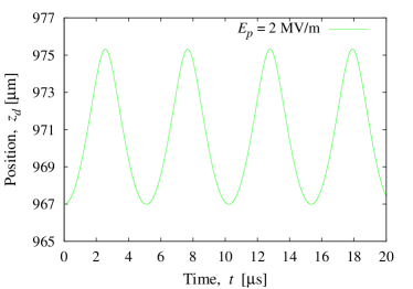
Figure 11: (Color online) Oscillating negatively charged nonrelativistic particle with structure in vicinity of the cathode. The $z_{d}\left(t\right)$ of Eq. (17) has been plotted using the initial value conditions defined in Eq. (22) and the parameter values defined in Eq. (9) with $\sigma_{1}=-0.012\,\textnormal{C}\cdot\textnormal{m}^{-2}$ and $V_{T}=2\,\textnormal{kV}$ (or $E_{p}=2\,\textnormal{MV}\cdot\textnormal{m}^{-1}$). The anode plate is located at $z_{d}=0\,\mu\textnormal{m}.$

II.2.2 Potential energy

The potential energy for a negatively charged particle subjected to the parallel plate electric field, $\mathbf{E}_{p},$ is obtained from Eq. (10) utilizing the line integral path illustrated in Fig. 7(b),

$$U\left(s\right)=-\int_{s_{\textnormal{ref}}}^{s}\mathbf{F}_{T}\cdot\mathbf{e}_{z}ds$$

or

$$U=-\int_{r_{2}}^{r_{1}}\mathbf{F}_{T}\cdot\mathbf{e}_{z}ds,$$ (23)

where, for convenience, $s_{\textnormal{ref}}$ and $s$ have been replaced by $r_{1}$ and $r_{2}$ illustrated in Fig. 7(b), respectively. Equivalently, Eq. (23) can be rewritten as

$$U=\int_{r_{1}}^{r_{2}}\mathbf{F}_{T}\cdot\mathbf{e}_{z}ds,$$ (24)

where the upper and the lower integral limits have been reversed. Multiplication of the both sides of Eq. (24) by a negative one yields

$$-U=-\int_{r_{1}}^{r_{2}}\mathbf{F}_{T}\cdot\mathbf{e}_{z}ds.$$ (25)

The right side of Eq. (25) can be obtained by making the following replacements in Eq. (12),

$$s_{\textnormal{ref}}\longrightarrow r_{1}\;\textnormal{ and }\;s\longrightarrow r_{2},$$

which yields

$$\int_{r_{1}}^{r_{2}}\mathbf{F}_{T}\cdot\mathbf{e}_{z}ds$$

$$=-\frac{\pi\epsilon_{0}\kappa_{3}\nu}{4}\left\{\frac{\nu}{r_{2}}+\frac{\nu}{h-r_{2}}+\frac{\left[\gamma\left(b^{3}-a^{3}\right)-b^{3}\right]E_{p}}{2r_{2}^{2}}\right.$$

$$\left.-\frac{\left[\gamma\left(b^{3}-a^{3}\right)-b^{3}\right]E_{p}}{2\left(h-r_{2}\right)^{2}}+8E_{p}r_{2}\right\}-mgr_{2}$$

$$+\frac{\pi\epsilon_{0}\kappa_{3}\nu}{4}\left\{\frac{\nu}{r_{1}}+\frac{\nu}{h-r_{1}}+\frac{\left[\gamma\left(b^{3}-a^{3}\right)-b^{3}\right]E_{p}}{2r_{1}^{2}}\right.$$

$$\left.-\frac{\left[\gamma\left(b^{3}-a^{3}\right)-b^{3}\right]E_{p}}{2\left(h-r_{1}\right)^{2}}+8E_{p}r_{1}\right\}+mgr_{1}.$$ (26)

Insertion of Eq. (26) into Eq. (24) yields

$$U =-\frac{\pi\epsilon_{0}\kappa_{3}\nu}{4}\left\{\frac{\nu}{r_{2}}+\frac{\nu}{h-r_{2}}+\frac{\left[\gamma\left(b^{3}-a^{3}\right)-b^{3}\right]E_{p}}{2r_{2}^{2}}\right.$$

$$\left.-\frac{\left[\gamma\left(b^{3}-a^{3}\right)-b^{3}\right]E_{p}}{2\left(h-r_{2}\right)^{2}}+8E_{p}r_{2}\right\}-mgr_{2}$$

$$+\frac{\pi\epsilon_{0}\kappa_{3}\nu}{4}\left\{\frac{\nu}{r_{1}}+\frac{\nu}{h-r_{1}}+\frac{\left[\gamma\left(b^{3}-a^{3}\right)-b^{3}\right]E_{p}}{2r_{1}^{2}}\right.$$

$$\left.-\frac{\left[\gamma\left(b^{3}-a^{3}\right)-b^{3}\right]E_{p}}{2\left(h-r_{1}\right)^{2}}+8E_{p}r_{1}\right\}+mgr_{1}.$$ (27)

For a negatively charged particle, $r_{1}=s$ and $r_{2}=s_{\textnormal{ref}};$ and, thus, Eq. (27) becomes

$$U\left(s\right) =-\frac{\pi\epsilon_{0}\kappa_{3}\nu}{4}\left\{\frac{\nu}{s_{\textnormal{ref}}}+\frac{\nu}{h-s_{\textnormal{ref}}}+\frac{\left[\gamma\left(b^{3}-a^{3}\right)-b^{3}\right]E_{p}}{2s_{\textnormal{ref}}^{2}}\right.$$

$$\left.-\frac{\left[\gamma\left(b^{3}-a^{3}\right)-b^{3}\right]E_{p}}{2\left(h-s_{\textnormal{ref}}\right)^{2}}+8E_{p}s_{\textnormal{ref}}\right\}-mgs_{\textnormal{ref}}$$

$$+\frac{\pi\epsilon_{0}\kappa_{3}\nu}{4}\left\{\frac{\nu}{s}+\frac{\nu}{h-s}+\frac{\left[\gamma\left(b^{3}-a^{3}\right)-b^{3}\right]E_{p}}{2s^{2}}\right.$$

$$\left.-\frac{\left[\gamma\left(b^{3}-a^{3}\right)-b^{3}\right]E_{p}}{2\left(h-s\right)^{2}}+8E_{p}s\right\}+mgs.$$ (28)

In terms of the $z_{d}$ parameter, i.e., $s=z_{d}+b,$ Eq. (28) becomes

$$U\left(z_{d}\right) =-\frac{\pi\epsilon_{0}\kappa_{3}\nu}{4}\left\{\frac{\nu}{s_{\textnormal{ref}}}+\frac{\nu}{h-s_{\textnormal{ref}}}+\frac{\left[\gamma\left(b^{3}-a^{3}\right)-b^{3}\right]E_{p}}{2s_{\textnormal{ref}}^{2}}\right.$$

$$\left.-\frac{\left[\gamma\left(b^{3}-a^{3}\right)-b^{3}\right]E_{p}}{2\left(h-s_{\textnormal{ref}}\right)^{2}}+8E_{p}s_{\textnormal{ref}}\right\}-mgs_{\textnormal{ref}}$$

$$+\frac{\pi\epsilon_{0}\kappa_{3}\nu}{4}\left\{\frac{\nu}{z_{d}+b}+\frac{\nu}{h-z_{d}-b}+\frac{\left[\gamma\left(b^{3}-a^{3}\right)-b^{3}\right]E_{p}}{2\left(z_{d}+b\right)^{2}}\right.$$

$$\left.-\frac{\left[\gamma\left(b^{3}-a^{3}\right)-b^{3}\right]E_{p}}{2\left(h-z_{d}-b\right)^{2}}+8E_{p}\left(z_{d}+b\right)\right\}$$

$$+mg\left(z_{d}+b\right).$$

As with the case of the positive particle, I shall set $s_{\textnormal{ref}}$ at the midway between the parallel plates, i.e., Eq. (14),

$$s_{\textnormal{ref}}=\frac{h}{2};$$

and, this yields

$$U\left(z_{d}\right) =\frac{\pi\epsilon_{0}\kappa_{3}\nu}{4}\left\{\frac{\nu}{z_{d}+b}+\frac{\nu}{h-z_{d}-b}\right.$$

$$+\frac{\left[\gamma\left(b^{3}-a^{3}\right)-b^{3}\right]E_{p}}{2\left(z_{d}+b\right)^{2}}-\frac{\left[\gamma\left(b^{3}-a^{3}\right)-b^{3}\right]E_{p}}{2\left(h-z_{d}-b\right)^{2}}$$

$$\left.+8E_{p}\left(z_{d}+b\right)\vphantom{\frac{\nu}{z_{d}+b}}\right\}+mg\left(z_{d}+b\right)$$

$$-\frac{\pi\epsilon_{0}\kappa_{3}\nu}{h}\left(\nu+E_{p}h^{2}\right)-\frac{1}{2}mgh,$$ (29)

where the resulting expression is, form wise, identical to the one in Eq. (15), i.e., the result corresponding to the case of positive particle.

Equation (29) is plotted for $\sigma_{1}=-0.012\,\textnormal{C}\cdot\textnormal{m}^{-2}$ with all other parameter values same as defined in Eq. (9),

$$\left\{\begin{array}[]{c}\kappa_{2}=6,\quad\kappa_{3}=1,\\ a=1.5\,\mu\textnormal{m},\quad h=1\,\textnormal{mm},\\ b-a=4\,\textnormal{nm},\\ V_{L}=0\,\textnormal{V},\\ \sigma_{2}=0\,\textnormal{C}\cdot\textnormal{m}^{-2}\textnormal{ (i.e., insulator)},\\ \rho_{m,1}=2700\,\textnormal{kg}\cdot\textnormal{m}^{-3},\\ \rho_{m,2}=3800\,\textnormal{kg}\cdot\textnormal{m}^{-3}.\end{array}\right.$$

For the plot, the anode voltages of $V_{T}=1\,\textnormal{kV},$ $V_{T}=2\,\textnormal{kV},$ and $V_{T}=3\,\textnormal{kV}$ are considered for comparison. For $V_{L}=0\,\textnormal{V}$ and $h=1\,\textnormal{mm},$ these anode voltages correspond to $E_{p}=1\,\textnormal{MV}\cdot\textnormal{m}^{-1},$ $E_{p}=2\,\textnormal{MV}\cdot\textnormal{m}^{-1},$ and $E_{p}=3\,\textnormal{MV}\cdot\textnormal{m}^{-1},$ respectively. The results are shown in Fig. 12.

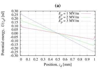
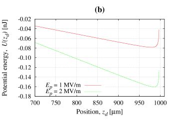
Figure 12: (Color online) (a) Plot of the potential energy function, $U\left(z_{d}\right)$ of Eq. (29), for $E_{p}=1\,\textnormal{MV}\cdot\textnormal{m}^{-1},$ $E_{p}=2\,\textnormal{MV}\cdot\textnormal{m}^{-1},$ and $E_{p}=3\,\textnormal{MV}\cdot\textnormal{m}^{-1}.$ The particle has a charge density of $\sigma_{1}=-0.012\,\textnormal{C}\cdot\textnormal{m}^{-2}$ and all other parameter values are as defined in Eq. (9). (b) Enlarged plot of $U\left(z_{d}\right)$ for domain $h/2<z_{d}<h,$ where $h=1\,\textnormal{mm}.$ In the plot, the anode is located at $z_{d}=0\,\mu\textnormal{m}.$

From the physical arguments based on the constituent forces, the oscillatory solutions for a negatively charged particle occur only in the domain $z_{d}>h/2$ in Figs. 12(a) and Fig. 12(b). The results show the potential well minima occurring in vicinity of the cathode side of the electrodes. Because the physical charged-particle cannot penetrate into the surface of the cathode, the parameter $z_{d}$ in Fig. 12(b) is bounded by $0\leq z_{d}\leq h-2b.$ The case of $z_{d}=h-2b$ corresponds to a situation in which the charged-particle is in physical contact with the cathode’s surface. There, the height of the potential well is finite and that criteria limits the width of the potential well, wherein the negatively charged particle can have oscillatory solutions. For instance, in the case of $E_{p}=1\,\textnormal{MV}\cdot\textnormal{m}^{-1}$ in Fig. 12(b), the width of the potential well is approximately $\sim 250\,\mu\textnormal{m};$ and, the oscillatory solutions exist approximately for $745\,\mu\textnormal{m}\lesssim z_{d}<996.99\,\mu\textnormal{m}.$ Similarly, for the case of $E_{p}=2\,\textnormal{MV}\cdot\textnormal{m}^{-1}$ in Fig. 12(b), the width of the potential well is approximately $\sim 125\,\mu\textnormal{m};$ and, the negatively charged particle is expected to have oscillatory solutions in a domain $\sim 872\,\mu\textnormal{m}\lesssim z_{d}<996.99\,\mu\textnormal{m}.$ For the negatively charged particle, the potential well, wherein the oscillatory solutions exist, gets formed in vicinity of the cathode. The width of such potential well decreases with increased $E_{p}.$ Physically, such property corresponds to the narrowing of the negative glow region with increased $E_{p}.$

II.3 Dipole radiation

II.3.1 Nonrelativistic regime

Oscillating charged-particle radiates electromagnetic energy. The power of such radiation, in the nonrelativistic limit, is given by Larmor radiation formula,

$$P_{rad}\left(t\right) =\frac{Q_{T}^{2}\ddot{z}_{d}^{2}}{6\pi\epsilon_{0}c^{3}},$$ (30)

where $\ddot{z}_{d}$ is the nonrelativistic charged-particle acceleration defined in Eq. (17), and $Q_{T}$ is the effective charge carried by the particle,Cho

$$Q_{T}=4\pi\epsilon_{0}\kappa_{3}\nu.$$ (31)

Insertion of Eqs. (17) and (31), respectively for $\ddot{z}_{d}$ and $Q_{T},$ into Eq. (30) yields

$$P_{rad}\left(t\right) =\frac{8\pi\epsilon_{0}\kappa_{3}^{2}\nu^{2}}{3c^{3}}\left(\frac{\pi\epsilon_{0}\kappa_{3}\nu}{4m}\left\{\frac{\nu}{\left(z_{d}+b\right)^{2}}\right.\right.$$

$$-\frac{\nu}{\left(h-z_{d}-b\right)^{2}}+\frac{\left[\gamma\left(b^{3}-a^{3}\right)-b^{3}\right]E_{p}}{\left(z_{d}+b\right)^{3}}$$

$$\left.\left.+\frac{\left[\gamma\left(b^{3}-a^{3}\right)-b^{3}\right]E_{p}}{\left(h-z_{d}-b\right)^{3}}-8E_{p}\right\}-g\right)^{2},$$ (32)

where $z_{d}$ is the solution to the Eq. (17).

I shall use the following parameter values to evaluate $P_{rad}\left(t\right):$

$$\left\{\begin{array}[]{c}\kappa_{2}=6,\quad\kappa_{3}=1,\\ a=25\,\textnormal{nm},\quad h=10\,\mu\textnormal{m},\\ b-a=2\,\textnormal{nm},\\ V_{T}=16\,\textnormal{kV},\quad V_{L}=0\,\textnormal{V},\\ \sigma_{1}=100\,\textnormal{C}\cdot\textnormal{m}^{-2},\\ \sigma_{2}=0\,\textnormal{C}\cdot\textnormal{m}^{-2}\textnormal{ (i.e., insulator)},\\ \rho_{m,1}=2700\,\textnormal{kg}\cdot\textnormal{m}^{-3},\\ \rho_{m,2}=3800\,\textnormal{kg}\cdot\textnormal{m}^{-3}.\end{array}\right.$$ (33)

The corresponding charged-particle motion is obtained by solving Eq. (17) via Runge-Kutta method. For the initial conditions, I shall choose

$$z_{d}\left(0\right)=1\,\mu\textnormal{m}\quad\textnormal{and}\quad\dot{z}_{d}\left(0\right)=0.$$ (34)

Illustrated in Figs. 13(a) and 13(b) are the results of $z_{d}\left(t\right)$ and $P_{rad}\left(t\right),$ respectively. The first sharp turning point in the plot of Fig. 13(a) has been enlarged and is shown in Fig. 13(c), where it shows the particle rebounding approximately at a distance of $10\,\textnormal{nm}$ from the anode plate electrode’s surface. The first pulse of the emitted Larmor radiation power has been enlarged and is shown in Fig. 13(d).

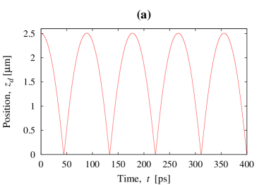
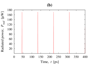
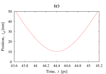
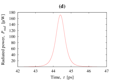
Figure 13: (Color online) (a) Plot of $z_{d}\left(t\right),$ Eq. (17), using the parameter values defined in Eq. (33) and the initial conditions defined in Eq. (34). (b) The corresponding Larmor radiation power computed from Eq. (32). (c) The first sharp turning point in (a) has been zoomed for a detailed view. (d) The first pulse in (b) has been zoomed for a detailed view. In the plot, the anode plate is located at $z_{d}=0\,\mu\textnormal{m}.$

Is $\sigma_{1}=100\,\textnormal{C}\cdot\textnormal{m}^{-2}$ experimentally an attainable surface charge density? The answer to this question is yes. In fact, for systems wherein nanoparticles are deliberately ionized in controlled manner, the surface charge density of $\sigma_{1}=100\,\textnormal{C}\cdot\textnormal{m}^{-2}$ is more reasonable than the one used in Eq. (9), i.e., $\sigma_{1}=0.012\,\textnormal{C}\cdot\textnormal{m}^{-2}.$ Physically, $\sigma_{1}=100\,\textnormal{C}\cdot\textnormal{m}^{-2}$ corresponds to a case wherein each aluminum atoms in the volume of radius $r=a$ contributing approximately one electron in the ionization process. This can be illustrated as follow. The mass of spherical aluminum core is

$$m_{c}=\frac{4}{3}\pi a^{3}\rho_{m,1};$$

and, the mass of a single aluminum atom is given by

$$m_{al}=\frac{m_{w}}{N_{A}},$$

where $m_{w}$ is the molar atomic weight and $N_{A}\approx 6.022\times 10^{23}\,\textnormal{mol}^{-1}$ is the Avogadro constant. The total number of aluminum atoms inside the volume of radius $r=a$ can be calculated as

$$N_{al}=\frac{m_{c}}{m_{al}}=\frac{4N_{A}\pi a^{3}\rho_{m,1}}{3m_{w}}.$$

The aluminum core of radius $r=a$ carries a surface charge of

$$Q_{sc}=4\pi a^{2}\sigma_{1}.$$

For a macroscopic particle, $Q_{sc}$ would be solely contributed from the atoms near the surface. However, for nanoparticles, the idea of “surface charge” becomes vague because it’s not just those atoms near the surface, but the atoms in the entire volume of nanoparticle that contribute to $Q_{sc}.$ In that sense, $Q_{sc}$ should be more appropriately coined as the “total charge” carried by the nanoparticle, albeit it is still defined in terms of the surface charge formula, $Q_{sc}=4\pi a^{2}\sigma_{1}.$ That said, how many electrons must be removed from each aluminum atoms in order for the core to have net positive charge in the amount of $Q_{sc}=4\pi a^{2}\sigma_{1}$? The answer to this question is

$$N_{e}=\frac{Q_{sc}}{q_{e}N_{al}}=\frac{3\pi\sigma_{1}m_{w}}{q_{e}N_{A}\pi a\rho_{m,1}},$$

where $q_{e}\approx 1.602\times 10^{-19}\,\textnormal{C}$ is the fundamental charge magnitude. For an aluminum atom, $m_{w}\approx 26.98\,\textnormal{g}$ and the number of electrons to be removed per aluminum atom is

$$N_{e}\approx 1.24\;\longrightarrow\;N_{e}=1,$$

where the greatest integer value has been taken for $N_{e},$ as there cannot be $1.24$ electrons, of course. This result implies that, on the average, each aluminum atoms in the core loses one electron during the ionization process in the case of $\sigma_{1}=100\,\textnormal{C}\cdot\textnormal{m}^{-2}$ and $a=25\,\textnormal{nm}.$

The anode voltage of $V_{T}=16\,\textnormal{kV}$ has been carefully chosen such that electrical breakdown does not occur between the parallel plates. Zouache and Lefort have demonstrated that by choosing a composite material for electrodes, for instance, composite material of $60\textnormal{\%}$ silver and $40\textnormal{\%}$ nickel, the DC bias voltage across the two electrodes can be as high as $3.85\,\textnormal{kV}$ at plate gap of $1\,\mu\textnormal{m}$ in vacuum before electrical breakdown takes place.IEEE-vacuum In terms of electric field strength, this corresponds to $E_{p}=3.85\,\textnormal{GV}\cdot\textnormal{m}^{-1}.$ At plate gap of $h=10\,\mu\textnormal{m}$ and the cathode grounded, the anode voltage of $V_{T}=16\,\textnormal{kV}$ corresponds to $E_{p}=1.6\,\textnormal{GV}\cdot\textnormal{m}^{-1},$ which is much less than $E_{p}=3.85\,\textnormal{GV}\cdot\textnormal{m}^{-1}.$

II.3.2 Relativistic regime

The Larmor radiation formula, Eq. (30), is only valid for particle speeds that are small relative to the speed of light. In the relativistic generalization, the total power radiated by oscillating charged-particle is given by the Liénard radiation formula,Cho

$$P_{rad}\left(t\right) =\frac{8\pi\epsilon_{0}\kappa_{3}^{2}\nu^{2}}{3c^{3}}\left[1-\left(\frac{\dot{z}_{d}}{c}\right)^{2}\right]^{-3}\ddot{z}_{d}^{2},$$ (35)

where $\ddot{z}_{d}$ is the particle’s acceleration associated with the relativistic force, Eq. (19). With the explicit expression for $\ddot{z}_{d}$ inserted from Eq. (21), the Liénard radiation formula of Eq. (35) becomes

$$P_{rad}\left(t\right) =\frac{8\pi\epsilon_{0}\kappa_{3}^{2}\nu^{2}}{3c^{3}}\left(\frac{\pi\epsilon_{0}\kappa_{3}\nu}{4m}\left\{\frac{\nu}{\left(z_{d}+b\right)^{2}}\right.\right.$$

$$-\frac{\nu}{\left(h-z_{d}-b\right)^{2}}+\frac{\left[\gamma\left(b^{3}-a^{3}\right)-b^{3}\right]E_{p}}{\left(z_{d}+b\right)^{3}}$$

$$\left.\left.+\frac{\left[\gamma\left(b^{3}-a^{3}\right)-b^{3}\right]E_{p}}{\left(h-z_{d}-b\right)^{3}}-8E_{p}\right\}-g\right)^{2},$$ (36)

which expression is identical to Eq. (32) with an exception that $z_{d}$ is now obtained from the relativistic dynamics, i.e., Eqs. (19) or (21).

III Mechanism for self-sustained oscillations in the positive glow corona

The typical configurations for the electrodes in the glow corona apparatus are illustrated in Fig. 14. When the potential difference between the rod shaped electrode and the plate electrode are sufficiently large, but not large enough to cause an electric arc, a glow occurs near the surface of the rod shaped electrode. For the case in which the rod shaped electrode is an anode, the glow corona is referred to as the positive glow corona whereas, if the rod shaped electrode is the cathode, the glow corona is referred to as the negative glow corona by convention. The schematics of the positive and the negative glow corona apparatuses are illustrated in Figs. 14(a) and 14(b), respectively. In this paper, only the positive glow corona is discussed.

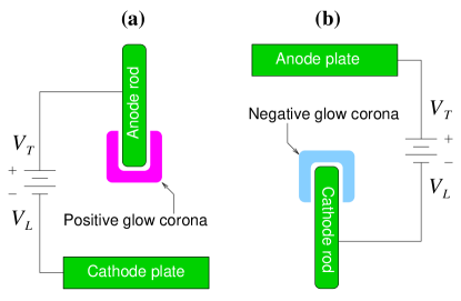
Figure 14: (Color online) (a) Schematic illustration of positive glow corona apparatus. In the positive glow corona, a glowing light is observed in vicinity of the anode. (b) Schematic illustration of a negative glow corona. In the negative glow corona, a glowing light is observed in vicinity of the cathode.

The first reported account with the glow corona is by Michael Faraday in 1838. However, only recently, people have begun to extensively investigate the phenomenon due to its potential applications in various scientific and engineering fields, such as semiconductor lithography, materials processing, plasma lighting, and so on.XUV Among the interesting properties of the phenomenon of glow corona, the self-sustained electrode current oscillations in the positive glow corona is the most extensively investigated one. Such self-sustained oscillations in the electrode current persists albeit the system as a whole is biased with a DC voltage across the electrodes. To this date, the basic underlying mechanism behind such self-sustained current oscillations remains unclear.corona-discharge-1 ; corona-discharge-2 ; corona-discharge-3 ; corona-discharge-4 ; corona-discharge-5

Morrow did a theoretical work in an attempt to explain the underlying physics behind the self-sustained current oscillations in the positive glow corona.corona-discharge-3 Qualitatively, his predictions are consistent with the various experimental observations by others. Despite the fact that plasmas are ionized gases,Bogaerts-DC-glow-discharge ; Gyergyek which may contain particles of all charged species (positive, negative, or neutral) of various sizes (atoms or nanoparticles), Morrow showed that the self-sustained oscillations in the electrode current are predominantly due to the mobility of the positive ions in the gas. He has calculated that approximately $96\%$ of the variations in the electrode current is due to the oscillations of the positive ions in the plasma. The current in the electrode can thus be expressed as

$$\mathbf{I}\left(t\right)\propto\sum_{n}Q_{T,n}\dot{\mathbf{z}}_{d,n}\left(t\right),$$

where $Q_{T,n}$ and $\dot{\mathbf{z}}_{d,n}\left(t\right)$ are the effective charge and the velocity of the $n\textnormal{th}$ charged-particle, respectively. In this paper, there is only one charged-particle; and, the expression for the electrode current becomes

$$\mathbf{I}\left(t\right)\propto Q_{T}\dot{\mathbf{z}}_{d}\left(t\right),$$

where $Q_{T}$ is the effective charge carried by the charged-particle and $\dot{\mathbf{z}}_{d}\left(t\right)$ is the charged-particle’s velocity. For the core-shell structured charged-particle considered here, the expression for $Q_{T}$ isCho

$$Q_{T}=8\pi a\left(b-a\right)\sigma_{1}\frac{\kappa_{3}}{\kappa_{2}}+4\pi\left(a^{2}\sigma_{1}+b^{2}\sigma_{2}\right),$$

which is a constant. Neglecting the constant terms, the current in the electrode becomes

$$\mathbf{I}\left(t\right)\propto\dot{\mathbf{z}}_{d}\left(t\right).$$ (37)

The $\dot{\mathbf{z}}_{d}\left(t\right)$ has been computed for the nonrelativistic charged-particle whose position versus time plot and the associated Larmor radiation power are illustrated in Figs. 13(a) and 13(b). The result is shown in Fig. 15(a), where the first abrupt rise in the velocity has been zoomed for a detailed view in Fig. 15(b). This result is compared with waveforms of experimental discharge current measurement at the electrode for a positive corona in nitrogen at 35 Torr by Akishev et al.corona-discharge-4 Similarly, the result is also compared with the prediction by Morrow.corona-discharge-3 Remarkably, the profile of Eq. (37), which is shown in Fig. 15(a), closely resembles both experimental and theoretical results by Akishev et al. and Morrow, respectively. For instance, the current in Eq. (37) has a saw-tooth shaped wave profile, which is qualitatively similar to the waveforms obtained by Akishev et al. and Morrow. Moreover, presented theory predicts pulses of radiation output occurring precisely at the point where the current rises abruptly. This can be checked from Figs. 13(b) and 15(a), where it shows pulses of radiation power coinciding with the abrupt rises in the charged-particle velocity versus time plot. Such characteristic is consistent with results obtained by Akishev et al. and Morrow. This shows that positive ion oscillations in the positive glow corona involve the kind of charged-particle oscillation mechanism discussed in Fig. 3.

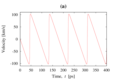
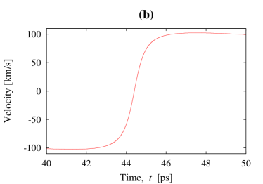
Figure 15: (Color online) (a) The plot of velocity, $\dot{\mathbf{z}}_{d}\left(t\right),$ corresponding to the charged-particle in Fig. 13. (b) The first abrupt rise in the velocity has been zoomed for a detailed view.

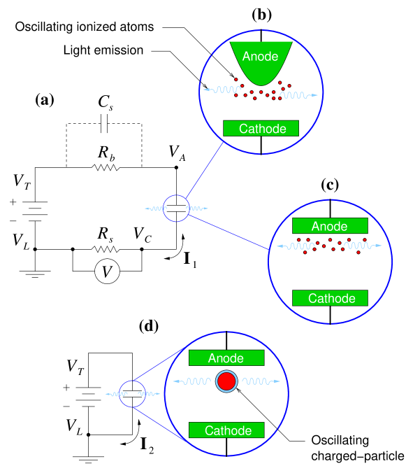
Figure 16: (Color online) (a) Typical experimental apparatus in the glow corona (or glow discharge) experiment. (b) Electrodes in the positive glow corona experiment. (c) Electrodes in the DC glow discharge experiment using parallel plates. The ballast resistor $R_{b}$ and the shunt resistor $R_{s}$ are shown. The voltmeter is placed across the shunt resistor. The $C_{s}$ is a stray capacity of external circuit. (d) The equivalent circuit diagram corresponding to the model in this paper.

The minor discrepancies in the electrode current waveforms between the result of this work and the experimental measurements by others can be attributed to the differences in the setup of the apparatus.corona-discharge-1 ; corona-discharge-2 ; corona-discharge-3 ; corona-discharge-4 ; corona-discharge-5 Illustrated in Fig. 16(a) is the equivalent circuit diagram representation for a typical apparatus in the glow corona experiments. The setup for a typical glow corona experiment involves the ballast resistor $R_{b},$ a shunt resistor $R_{s},$ and a stray capacitance $C_{s}$ from the external circuit. In the positive glow corona experiment,corona-discharge-4 the typical geometry for the anode and cathode electrodes are as illustrated in Fig. 16(b) whereas, in a typical DC glow discharge experiments, the parallel plate geometry, such as the one illustrated in Fig. 16(c), is the typical configuration for the electrodes.Kuschel-axial-light The presence of the ballast and the shunt resistors in the circuit keeps the anode at voltage $V_{A}\left(t\right)$ and the cathode at voltage $V_{C}\left(t\right).$

These configurations for the glow corona experiment, Figs. 16(a)-16(c), are compared with the model configuration considered in this work, Fig. 4. The equivalent circuit diagram for the model illustrated in Fig. 4 is as shown in Fig. 16(d). Unlike the typical setup in the glow corona (or DC glow discharge) experiments, the equivalent circuit diagram for the model considered here does not contain the ballast and the shunt resistors in the circuit. Absence of these resistors in the circuit keep the anode and the cathode voltages fixed, respectively, at $V_{T}$ and $V_{L}$ in Fig. 4. Contrary to this, the anode and the cathode voltages in a typical glow corona experiment are not fixed at some constant values due to the presence of the ballast and the shunt resistors. For instance, the voltages $V_{A}\left(t\right)$ and $V_{C}\left(t\right)$ in Fig. 16(a) are not constants, but vary in time due to the dynamics of ionized atoms in the space between the anode and the cathode electrodes. For this reason, the electrode voltage oscillation measurements from an experiment, in which the setup is equivalent to the one illustrated in Fig. 16(a), cannot be used directly to test the theory presented in this paper. However, the current oscillations in the electrodes are present in all of the configurations in Fig. 16. For instance, an oscillating ionized particle between the anode and the cathode gives rise to an electrode current, $\mathbf{I}_{1}\left(t\right)$ in Fig. 16(a) and $\mathbf{I}_{2}\left(t\right)$ in Fig. 16(d), which oscillates in correlation to the motion of oscillating ionized particle. Such electrode current oscillations get induced in the circuit regardless of whether the ballast and the shunt resistors are present in the circuit or not. The electrode current oscillation measurements from Figs. 16(a)-16(c), therefore, can be used to test the theory presented here; and, this is essentially what was assumed in Eq. (37).

Since the geometry of the anode used in the experiment is different from the simple plate geometry assumed in the model adopted in this paper, the resulting waveforms of oscillating electrode currents from this theory, $\mathbf{I}_{2}\left(t\right),$ and the experiment, $\mathbf{I}_{1}\left(t\right),$ are not identical. Nevertheless, qualitatively, both $\mathbf{I}_{1}\left(t\right)$ and $\mathbf{I}_{2}\left(t\right)$ show the same characteristic behavior. This must be so because the basic mechanism behind the oscillations in $\mathbf{I}_{1}\left(t\right)$ and $\mathbf{I}_{2}\left(t\right)$ originates from the same physics. One such characteristic behavior is the presence of radiation output accompanying the abrupt rises in the $\mathbf{I}_{1}\left(t\right)$ and $\mathbf{I}_{2}\left(t\right),$ which was discussed previously from Figs. 13(b) and 15(a).

Besides the geometrical differences in the anode, the model treated here has only a single charged-particle in the space between the anode and the cathode whereas, in the glow corona experiments,corona-discharge-1 ; corona-discharge-2 ; corona-discharge-4 the space between the electrodes is filled with an ionized gas, i.e., many ionized atoms. Despite these differences, the theory qualitatively reproduces the self-sustained current oscillations in the electrode, consistent with the results from the various glow corona experiments. Such result suggests that the phenomenon of self-sustained electrode current oscillations in the positive glow corona is a manifestation of the charged-particle oscillation discussed in this paper.

The radiation power in Fig. 13(b) is emitted at frequency of approximately $10\,\textnormal{GHz},$ which is not a visible light. How can the pulses of light accompanying the saw-tooth shaped electrode current oscillations be explained? To answer this, typical glow corona experiment involves gases. There, individual atoms can be highly ionized to oscillate at frequencies large enough to emit visible light. The plasma as a whole, however, oscillates at much smaller frequencies because its dynamics involves the collective motions of all constituent ionized atoms. This qualitatively explains the pulses of light accompanying the self-sustained electrode current oscillations, which oscillates at much lower frequencies.

As an extension of this theory, the self-sustained oscillations in the negative glow corona, Fig. 14b, can be qualitatively explained from the negatively charged particles going through an oscillatory motion in vicinity of the cathode, which is schematically illustrated in Fig. 10. The neon lamp used in the Pearson–Anson relaxation oscillator is the classic example of negative glow corona at work. When the neon bulb is biased with a direct current (DC) voltage, typically around $60\,\textnormal{V},$ a glow gets formed around the cathode lead. No such glow occurs near the anode lead. It is unlikely that neon atoms inside the lamp are positively charged. Quantum mechanical calculations show that it takes minimum electric field strength of approximately $4.8\,\textnormal{V}\cdot\textnormal{\r{A}}^{-1}$ (or $48\,\textnormal{GV}\cdot\textnormal{m}^{-1}$) to strip an electron from a neon at temperature of $273^{\text{\textdegree}}\textnormal{K}.$field-emission-neon In a typical neon bulbs used in the Pearson-Anson relaxation oscillators, the anode and the cathode leads are separated by a gap of just few millimeters. Assuming a gap of $1\,\textnormal{mm}$ between the electrodes, and a DC bias voltage of $60\,\textnormal{V},$ the electric field between the electrodes is $60\,\textnormal{kV}\cdot\textnormal{m}^{-1}.$ This electric field is not large enough to ionize a neon atom. However, an electric field of $60\,\textnormal{kV}\cdot\textnormal{m}^{-1}$ at relatively warm temperature is sufficient to emit electrons from the surface of the cathode lead. Because neon is highly electronegative, it attracts any free electrons nearby and becomes negatively charged.electronegativity Such case, in which a negatively charged neon atom oscillates in vicinity of the cathode, is qualitatively explained by the theory presented in this paper.

IV Concluding Remarks

The self-sustained electrode current oscillations in the positive glow corona can be qualitatively explained by the oscillatory solutions which is quite naturally obtained from the associated electromagnetic boundary value problem. To demonstrate this, a simple, DC voltage biased, plane-parallel plate system with a charged-particle inside has been considered. The resulting oscillatory solutions for the charged-particle motion qualitatively explains the observed experimental results. The remarkable similarities in the waveforms of the self-sustained electrode current oscillations between the various experimentscorona-discharge-1 ; corona-discharge-2 ; corona-discharge-4 and the prediction from this work indicate that the basic underlying mechanism behind the self-sustained oscillations in the positive glow corona involves the kind of push-pull mechanism discussed in Fig. 3.

V Acknowledgments

The author acknowledges the support for this work provided by Samsung Electronics Co., Ltd.

References

(1) J. Jackson, Classical Electrodynamics - Third
Edition, Ch. 2 (John Wiley & Sons, Inc., 1998).
(2) M. Goldman, A. Goldman, and R. Sigmond,
Pure & Appl. Chem. 57(9), 1353-1362 (1985).
(3) R. Sigmond, J. Phys. IV France 7,
C4-383 (1997)
(4) R. Morrow, J. Phys. D: Appl. Phys.
30, 3099 (1997).
(5) Yu. Akishev, M. Grushin, A. Deryugin,
A. Napartovich, M. Pan’kin, and N. Trushkin, J. Phys. D: Appl. Phys.
32, 2399 (1999).
(6) N. Allen, M. Abdel-Salam, M. Boutlendj,
I. Cotton, and B. Tan, IET Sci. Meas. Technol.1(2),
103 (2007).
(7) S. Cho, Phys. Plasmas 19(3), 033506 (2012).
(8) K. Tamura, Y. Kimura, H. Suzuki, O. Kido, T.
Sato, T. Tanigaki, M. Kurumada, Y. Saito, and C. Kaito, Jpn. J. Appl.
Phys. 42, 7489 (2003).
(9) R. Sohal, G. Lupina, O. Seifarth, P. Zaumseil, and
C. Walczyk, Surface Science 604, 276 (2010).
(10) N. Zouache and A. Lefort, IEEE Trans. Dielectr.
Electr. Insul. 4(4), 358 (1997).
(11) T. Higashiguchi, H. Terauchi, N. Yugami, T. Yatagai,
W. Sasaki, R. D’Arcy, P. Dunne, and G. O’Sullivan, Appl. Phys. Lett.
96(13), 131505 (2010).
(12) A. Bogaerts, E. Neyts, R. Gijbels,
and Joost. van der Mullen, Spectrochimica Acta Part B57(4),
609 (2002).
(13) T. Gyergyek, M. Čerček, M. Stanojević,
and N. Jelić, J. Phys. D: Appl. Phys. 27, 2080 (1994).
(14) T. Kuschel, B. Niermann, I. Stefanović,
M. Böke, N. Škoro, D. Marić, Z. Petrović, and J. Winter, Plasma
Sources Sci. Technol. 20, 065001 (2011).
(15) D. Brandon, Br. J. Appl. Phys. 14,
474 (1963).
(16) N. Islam and D. Ghosh, J. of Quantum
Information Science 1, 135 (2011).