Search for Solar Axions Produced in $p(d,\rm{{}^{3}He})A$ Reaction with Borexino Detector

Abstract

¹ Dipartimento di Fisica, Universita’ degli Studi e INFN, 20133 Milano, Italy

² Chemical Engineering Department, Princeton University, Princeton, NJ 08544, USA

³ Institut fur Experimentalphysik, Universitat, 22761 Hamburg, Germany

⁴ INFN Laboratori Nazionali del Gran Sasso, SS 17 bis Km 18+910, 67010 Assergi (AQ), Italy

⁵ Physics Department, Virginia Polytechnic Institute and State University, Blacksburg, VA 24061, USA

⁶Physics Department, University of Massachusetts, Amherst, AM01003, USA

⁷ Physics Department, Princeton University, Princeton, NJ 08544, USA

⁸ Dipartimento di Fisica, Universita’ e INFN, Genova 16146, Italy

⁹St. Petersburg Nuclear Physics Institute, 188350 Gatchina, Russia

¹⁰ NRC Kurchatov Institute, 123182 Moscow, Russia

¹¹ Joint Institute for Nuclear Research, 141980 Dubna, Russia

¹² Laboratoire AstroParticule et Cosmologie, 75231 Paris cedex 13, France

¹³ Physik Department, Technische Universitaet Muenchen, 85747 Garching, Germany

¹⁴ Max-Plank-Institut fuer Kernphysik, 69029 Heidelberg, Germany

¹⁵M. Smoluchowski Institute of Physics, Jagellonian University, 30059 Krakow, Poland

¹⁶Dipartimento di Chimica, Universita’ e INFN, 06123 Perugia, Italy

Borexino collaboration

A search for 5.5-MeV solar axions produced in the $p+d\rightarrow\rm{{}^{3}He}+A~{}(5.5\rm{~{}MeV})$ reaction was performed using the Borexino detector. The Compton conversion of axions to photons, ${\rm A}+e\rightarrow e+\gamma$; the axio-electric effect, ${\rm A}+e+Z\rightarrow e+Z$; the decay of axions into two photons, ${\rm A}\rightarrow 2\gamma$; and inverse Primakoff conversion on nuclei, ${\rm A}+Z\rightarrow\gamma+Z$, are considered. Model independent limits on axion-electron ($g_{Ae}$), axion-photon ($g_{A\gamma}$), and isovector axion-nucleon ($g_{3AN}$) couplings are obtained: $|g_{Ae}\times g_{3AN}|\leq 5.5\times 10^{-13}$ and $|g_{A\gamma}\times g_{3AN}|\leq 4.6\times 10^{-11}\rm{GeV}^{-1}$ at $m_{A}<$ 1 MeV (90% c.l.). These limits are 2-4 orders of magnitude stronger than those obtained in previous laboratory-based experiments using nuclear reactors and accelerators.

I INTRODUCTION

The axion hypothesis was introduced by Weinberg Wei78 and Wilczek Wil78 , who showed that the solution to the problem of $CP$ conservation in strong interactions, proposed earlier by Peccei and Quinn Pec77 , should lead to the existence of a neutral pseudoscalar particle. The original WWPQ axion model produced specific predictions for the coupling constants between axions and photons ($g_{A\gamma}$), electrons ($g_{Ae}$), and nucleons ($g_{AN}$) which were soon disproved by experiments performed with reactors and accelerators, and by experiments with artificial radioactive sources PDG10 .

Two classes of new theoretical models, hadronic or KSVZ Kim79 ; Shi80 and GUT or DFSZ Zhi80 ; Din81 , describe ”invisible” axions, which solve the $CP$ problem in strong interactions and interact more weakly with matter. The scale of Peccei-Quinn symmetry violation ($f_{A}$) in both models is arbitrary and can be extended to the Planck mass $m_{P}\approx 10^{19}$ GeV. The axion mass in these models is determined by the axion decay constant $f_{A}$:

$$m_{A}\approx(f_{\pi}m_{\pi}/f_{A})(\sqrt{z}/(1+z)),$$ (1)

where $m_{\pi}$ and $f_{\pi}$ are, respectively, the mass and decay constant of the neutral $\pi$ meson and $z=m_{u}/m_{d}$ is $u$ and $d$ quark-mass ratio. The equation (1) can be rewritten as: $m_{A}(\rm{eV})\approx 6.0\times 10^{6}/\it{f_{A}}{\rm{(GeV)}}$. Since the axion -hadron and axion -lepton interaction amplitudes are proportional to the axion mass, the interaction between axions and matter is suppressed.

The effective coupling constants $g_{A\gamma}$, $g_{Ae}$, and $g_{AN}$ are to a great extent model dependent. For example, the hadronic axion cannot interact directly with leptons, and the constant $g_{Ae}$ exists only because of radiative corrections. Also, the constant $g_{A\gamma}$ can differ by more than two orders of magnitude from the values accepted in the KSVZ and DFSZ models Kap85 .

The results from present-day experiments are interpreted within these two most popular axion models. The main experimental efforts are focused on searching for an axion with a mass in the range of $10^{-6}$ to $10^{-2}$ eV. This range is free of astrophysical and cosmological constraints, and relic axions with such a mass are considered to be the most likely dark matter candidates.

New solutions to the $CP$ problem rely on the hypothesis of a world of mirror particles Bere00 ; Bere01 and super-symmetry Hal04 . These models allow the existence of axions with a mass of about 1 MeV, which are not precluded by laboratory experiments or astrophysical data.

The purpose of this study is to search experimentally for solar axions with an energy of 5.5 MeV, produced in the $p+d\rightarrow\rm{{}^{3}He}+A$ (5.49 MeV) reaction. The axion flux is thus proportional to the $pp$-neutrino flux, which is known with a high accuracy Ser09 ; Bel11A . The range of axion masses under study has been extended to 5 MeV. The axion detection signatures exploited in this study are Compton axion to photon conversion, ${\rm A}+e\rightarrow e+\gamma$, and the axio-electric effect, ${\rm A}+e+Z\rightarrow e+Z$. The amplitudes of these processes are defined by the $g_{Ae}$ coupling. We also consider the potential signals from axion decay into two $\gamma$-quanta and from inverse Primakoff conversion on nuclei, ${\rm A}+Z\rightarrow\gamma+Z$. The amplitudes of these reactions depend on the axion-photon coupling $g_{A\gamma}$. The signature of all these reactions is a 5.5 MeV peak.

We have previously published a search for solar axions emitted in the 478 keV M1-transition of ${}^{7}{\rm{Li}}$ using the Borexino counting test facility Bel08 .

The results of laboratory searches for the axion as well as astrophysical and cosmological axion bounds can be found in PDG10 .

II The flux of 5.5 MeV axions

The Sun potentially represents an efficient and intense source of axions. One production mechanism is photon -axion conversion in the electromagnetic fields of the solar plasma. In addition, electrons could produce axions via Compton processes and bremsstrahlung. Finally, monochromatic axions could be emitted in magnetic transitions in nuclei, when low-lying levels are thermally excited by the high temperature of the Sun.

Even the reactions of the pp-solar fusion chain and the CNO cycle can produce axions. The most intense flux is expected from the formation of the $\rm{{}^{3}He}$ nucleus:

$$p+d\rightarrow\rm{{{}^{3}He}+\gamma~{}(5.5\;MeV)}.$$ (2)

According to the Standard Solar Model (SSM), 99.7% of all deuterium is produced from the fusion of two protons, $p+p\rightarrow d+e^{+}+\nu_{e}$, while the remaining 0.3% is due to the $p+p+e^{-}\rightarrow d+\nu_{e}$ reaction. The produced deuteron captures a proton with lifetime $\tau=6s$.

The expected solar axion flux can thus be expressed in terms of the $pp$-neutrino flux. The proportionality factor between the axion and neutrino fluxes is determined by a dimensionless axion-nucleon coupling constant $g_{AN}$, which consists of isoscalar $g_{0AN}$ and isovector $g_{3AN}$ components. The ratio between the probability of an M1 magnetic nuclear transition with axion production $(\omega_{A})$ and photon production $(\omega_{\gamma})$ can be expressed as Hax91 -Avi88 :

$$\frac{\omega_{A}}{\omega_{\gamma}}=\frac{1}{2\pi\alpha}\frac{1}{1+\delta^{2}}\left[\frac{g_{0AN}\beta_{1}+g_{3AN}}{(\mu_{0}-0.5)\beta_{1}+\mu_{3}-\eta_{1}}\right]^{2}\left(\frac{p_{A}}{p_{\gamma}}\right)^{3},$$ (3)

where $p_{\gamma}$ and $p_{A}$ are, respectively, the photon and axion momenta; $\delta^{2}=E/M$ is the ratio between the probabilities of $E$ and $M$ transitions; $\alpha\approx 1/137$ is the fine-structure constant; $\mu_{0}=\mu_{p}+\mu_{n}\approx 0.88$ and $\mu_{3}=\mu_{p}-\mu_{n}\approx 4.71$ are, respectively, the isoscalar and isovector nuclear magnetic moments; and $\beta_{1}$ and $\eta_{1}$ are parameters dependent on the specific nuclear matrix elements.

Within the hadronic axion model, the constants $g_{0AN}$ and $g_{3AN}$ can be written in terms of the axion mass Kap85 ,Sre85 :

$$g_{0AN}=-\frac{m_{N}}{6f_{A}}[2S_{fs}+(3F-D)\frac{1+z-2w}{1+z+w}]=$$

$$=-4.03\times 10^{-8}(m_{A}/1{\rm{eV}}),$$ (4)

$$g_{3AN}=-\frac{m_{N}}{2f_{A}}[(D+F)\frac{1-z}{1+z+w}]=$$

$$=-2.75\times 10^{-8}(m_{A}/1{\rm{eV}}).$$ (5)

where $m_{N}\approx 939$ MeV is the nucleon mass, and $z=m_{u}/m_{d}\cong 0.56$ and $w=m_{u}/m_{s}\cong 0.029$ are $u$, $d$ and $s$ quark-mass ratios. Axial-coupling parameters $F$ and $D$ are obtained from hyperon semi-leptonic decays with high precision: $F$=0.462 $\pm$ 0.011, $D$= 0.808 $\pm$ 0.006 Mat05 . The parameter $S_{fs}$, characterizing the flavor singlet coupling is poorly constrained: $(0.37\leq S_{fs}\leq 0.53)$ and $(0.15\leq S_{fs}\leq 0.5)$ were found in Alt97 and Ada97 , respectively. The values of the axion-nucleon couplings given in (4) and (5) are obtained assuming $S_{fs}$=0.5. The value of $u$- and $d$-quark-mass ratio $z$ = 0.56 is generally accepted for axion papers, but it could vary in the range ($0.35-0.6$) PDG10 . These uncertainties in $S_{fs}$ and $z$ could cause the values of $g_{0AN}$ and $g_{3AN}$ to differ from (4) and (5) by factors of (0.4–1.3) and (0.9–1.9) times, respectively.

The values of $g_{0AN}$ and $g_{3AN}$ in the DFSZ model depend on an additional unknown parameter, but have the same order of magnitude: they have ($0.3-1.5$) times the values of the corresponding constants for the hadronic axion.

Figure 1: Ratio of the emission probabilities for axions and $\gamma$ quanta ($\omega_{A}/\omega_{\gamma}$) in the $p+d\rightarrow{{}^{3}{\rm{He}}}+\gamma$ reaction (curve 1, left-hand scale); cross section of the Compton conversion and axio-electric effect for 5.5-MeV axions on carbon atoms for $g_{Ae}=1$ (curve 2 and 3, right-hand scale).

In the $p+d\rightarrow\rm{{}^{3}He}+\gamma$ reaction, the M1-type transition corresponds to the capture of a proton with zero orbital momentum. The probability, $\chi$, of proton capture from the $S$ state at energies below 80 keV was measured in Sch97 ; at a proton energy of $\sim 1$ keV, $\chi$ = 0.55 $(\delta^{2}=0.82)$. The proton capture from the $S$ state corresponds is an isovector transition, and the ratio $\omega_{A}/\omega_{\gamma}$, from expression (3), therefore depends only on $g_{3AN}$ Don78 :

$$\frac{\omega_{A}}{\omega_{\gamma}}=\frac{\chi}{2\pi\alpha}\left[\frac{g_{3AN}}{\mu_{3}}\right]^{2}\left(\frac{p_{A}}{p_{\gamma}}\right)^{3}=0.54(g_{3AN})^{2}\left(\frac{p_{A}}{p_{\gamma}}\right)^{3}.$$ (6)

The calculated values of the $\omega_{A}/\omega_{\gamma}$ ratio as a function of the axion mass are shown in Fig.1. The expected solar axion flux on the Earth’s surface is then

$$\Phi_{A0}=\Phi_{\nu pp}(\omega_{A}/\omega_{\gamma})=3.23\times 10^{10}(g_{3AN})^{2}(p_{A}/p_{\gamma})^{3},$$ (7)

where $\Phi_{\nu pp}=6.0\times 10^{10}{\rm{cm}}^{-2}{\rm{s}}^{-1}$ is the $pp$ solar neutrino flux Ser09 ; Bel11A . Using the relation between $g_{3AN}$ and $m_{A}$ given by (II), the $\Phi_{A0}$ value appears to be proportional to $m_{A}^{2}$: $\Phi_{A0}=2.44\times 10^{-5}m_{A}^{2}(p_{A}/p_{\gamma})^{3}$, where $m_{A}$ is given in eV units.

III INTERACTION OF AXIONS WITH MATTER AND AXION DECAYS

III.1 Axion-electron interactions: Compton conversion and the axio-electric effect

An axion can scatter an electron to produce a photon in the Compton-like process $A+e\rightarrow\gamma+e$. The Compton differential cross section for electrons was calculated in Don78 , Avi88 , Zhi79 . The energy spectrum of the $\gamma$-quanta depends on the axion mass, while the spectra of electrons can be found from relation $E_{e}=E_{A}-E_{\gamma}$. Here, $E_{A}\cong$ 5.49 MeV, which is the Q-value of the $p(d,\rm{{}^{3}He})\gamma$ reaction. The integral cross section corresponding to this mode is Don78 , Avi88 , Zhi79 :

$$\sigma_{CC}=\frac{g_{Ae}^{2}\alpha}{8m^{2}p_{A}}[\frac{2m^{2}(m+E_{A})y}{(m^{2}+y)^{2}}+$$

$$+\frac{4m(m_{A}^{4}+2m_{A}^{2}m^{2}-4m^{2}E_{A}^{2})}{y(m^{2}+y)}+$$

$$+\frac{4m^{2}p_{A}^{2}+m_{A}^{4}}{p_{A}y}\ln\frac{m+E_{A}+p_{A}}{m+E_{A}-p_{A}}].$$ (8)

where $p_{A}$ and $E_{A}$ are the momenta and the energy of the axion respectively and $y=2mE_{A}+m_{A}^{2}$. The dimensionless coupling constant $g_{Ae}$ is associated with the electron mass $m$, so that $g_{Ae}=C_{e}m/f_{A}$, where $C_{e}$ is a model dependent factor of the order of unity. In the standard WWPQ axion model, the values $f_{A}$=250 GeV and $C_{e}$=1 are fixed and $g_{Ae}\approx 2\times 10^{-6}$. In the DFSZ axion models $C_{e}=1/3\cos^{2}\beta_{\rm{dfsz}}$, where $\beta_{\rm{dfsz}}$ is an arbitrary angle. Assuming $\cos^{2}\beta_{\rm{dfsz}}$=1, the axion-electron coupling is $g_{Ae}$=2.8$\times 10^{-11}m_{A}$ where $m_{A}$ is expressed in $eV$ units. The hadronic axion has no tree-level couplings to the electron, but there is an induced axion-electron coupling at one-loop level Sre85 :

$$g_{Ae}=\frac{3n\alpha^{2}m}{2\pi f_{a}}\left(\frac{E}{N}\ln\frac{f_{A}}{m}-\frac{2}{3}\frac{4+z+w}{1+z+w}\ln\frac{\Lambda}{m}\right)$$ (9)

where $n$ is the number of generations, $N$ and $E$ are the model dependent coefficients of the color and electromagnetic anomalies and $\Lambda\approx$1 GeV is the cutoff at the QCD confinement scale. The interaction strength of the hadronic axion with the electron is suppressed by a factor $\sim\alpha^{2}$.

The integral cross section $\sigma_{CC}$ calculated for $g_{Ae}=1$ is shown in Fig.1. For axions with fixed $g_{Ae}$ (curve 2 in Fig. 1), the phase space contribution to the cross section is approximately independent of $m_{A}$ for $m_{A}<$ 2 MeV and the integral cross section is:

$$\sigma_{CC}\approx g_{Ae}^{2}\times 4.3\times 10^{-25}\rm{cm^{2}}.$$ (10)

The other process associated with axion-electron coupling is the axio-electric effect $A+e+Z\rightarrow e+Z$ (the analogue of the photo-electric effect). In this process the axion disappears and an electron is emitted from an atom with an energy equal to the energy of the absorbed axion minus the electron binding energy $E_{b}$. The cross section of the axio-electric effect on K-electrons where the axion energy $E_{A}\gg E_{b}$ was calculated in Zhi79 and has a complex form; it is shown in Fig. 1. The cross section has a $Z^{5}$ dependence and for carbon atoms the cross section is $\sigma_{Ae}\approx g_{Ae}^{2}\times$1.3$\times$10^-29 cm²/electron for $m_{A}<$ 1 MeV. This value is more than 4 orders of magnitude lower than for axion Compton conversion. However, thanks to the different energy dependence ($\sigma_{CC}\sim E_{A}$, $\sigma_{Ae}\sim(E_{A})^{-3/2}$) and $Z^{5}$ dependence, the axio-electric effect is a potential signature for axions with detectors having high $Z$ active mass Der10 .

For axions with a mass above $2m$, the main decay mode is the decay into an electron-positron pair: $A\rightarrow e^{+}+e^{-}$. The lifetime of an axion in the intrinsic reference system has the form:

$$\tau_{e^{+}e^{-}}=8\pi/(g^{2}_{Ae}\sqrt{m^{2}_{A}-4m^{2}_{e}}).$$ (11)

The probability of an axion to reach the Earth is

$$P(m_{A},p_{A})=\exp(-\tau_{f}/\tau_{e^{+}e^{-}}),$$ (12)

where $\tau_{f}$ is the time of flight in the reference system associated with the axion:

$$\tau_{f}=\frac{Lm_{A}}{cp_{A}}=\frac{m_{A}}{E_{A}}\frac{L}{\beta c}.$$ (13)

Here $L=1.5\times 10^{13}$ cm is the distance from the Earth to the Sun and $\beta=p_{A}/E_{A}$ is the axion velocity in terms of the speed of light. The condition $\tau_{f}<0.1\tau_{e^{+}e^{-}}$ (in this case, $90\%$ of all axions reach the Earth) limits the sensitivity of solar axion experiments to $g_{Ae}<(10^{-12}-10^{-11})$ Der10 .

III.2 Axion-photon interaction: axion decay and the inverse Primakoff conversion on nuclei

If the axion mass is less than $2m$, $A\rightarrow e^{+}+e^{-}$ decay is forbidden, but the axion can decay into two $\gamma$ quanta. The probability of the decay, which depends on the axion -photon coupling constant and the axion mass, is given by the expression:

$$\tau_{2\gamma}=\frac{64\pi}{g_{A\gamma}^{2}m_{A}^{3}}.$$ (14)

where $g_{A\gamma}$ is an axion-photon coupling constant with dimension of (energy)^-1 which is presented as in Kap85 ,Sre85 :

$$g_{A\gamma}=\frac{\alpha}{2\pi f_{A}}\left(\frac{E}{N}-\frac{2(4+z+w)}{3(1+z+w)}\right)\equiv\frac{\alpha}{2\pi f_{A}}C_{A\gamma\gamma}$$ (15)

where $E/N$ is a model dependent parameter of the order of unity. $E/N$ = 8/3 in the DFSZ axion models ($C_{A\gamma\gamma}$=0.74) and $E/N$ = 0 for the original KSVZ axion ($C_{A\gamma\gamma}$=-1.92).

The phase space for decay depends on $m_{A}^{3}$. For $\tau_{2\gamma}$ measured in seconds, $g_{A\gamma}$ in ${\rm GeV^{-1}}$, and $m_{A}$ in ${\rm eV}$, one obtains:

$$\tau_{2\gamma}=1.3\times 10^{5}g_{A\gamma}^{-2}m_{A}^{-3}=3.5\times 10^{24}m_{A}^{-5}C_{A\gamma\gamma}^{-2}.$$ (16)

The flux of axions reaching the detector is given by

$$\Phi_{A}={\rm{exp}}(-\tau_{f}/\tau_{2\gamma})\Phi_{A0}={\rm{exp}}(-\tau_{f}g_{A\gamma}^{2}m_{A}^{3}/64\pi)\Phi_{A0}$$ (17)

where $\Phi_{A0}$ is the axion flux at the at the Earth in case there is no axion decay (7), $\tau_{2\gamma}$ is defined by (14, 16), and $\tau_{f}$, given by (13) is the time of flight in the axion frame of reference. Because of axion decay, the sensitivity of experiments using solar axions drops off for large values of $g_{A\gamma}^{2}m_{A}^{3}$.

The number of $A\rightarrow 2\gamma$ decays in a detector of volume V is:

$$N_{\gamma}=\Phi_{A}\frac{Vm_{A}}{\beta cE_{A}\tau_{2\gamma}}.$$ (18)

This leads, using the KSVZ model, to expected Borexino event rates like those shown in Fig.2 for different values of $m_{A}$. As can be seen in the Figure, the expected event rate is peaked, with a drop-off at low $m_{A}$ due to the lower axion decay rate in the detector, and a decrease at high $m_{A}$ resulting from the reduced flux from axion decay in flight. The maximum $N_{\gamma}$ corresponds to $m_{A}$ = $((8/6)\tau_{2\gamma}m_{A}^{5}/(\tau_{f}/m_{A}))^{1/6}$= 65 keV, where $\tau_{2\gamma}$ and $\tau_{f}$ are defined by (16) and (13).

Another process depending on $g_{A\gamma}$ coupling is the Primakoff photo-production on carbon nuclei $A+{{}^{12}\rm{C}}\rightarrow\gamma+{{}^{12}\rm{C}}$. The integral inverse Primakoff conversion cross section is Avi88 :

$$\sigma_{PC}=g_{A\gamma}^{2}\frac{Z^{2}\alpha}{2}\left[\frac{1+\beta^{2}}{2\beta^{2}}\ln\left(\frac{1+\beta}{1-\beta}\right)-\frac{1}{\beta}\right].$$ (19)

Because the cross section depends on the $g_{A\gamma}$ coupling, the decrease in the axion flux due to $A\rightarrow 2\gamma$ decays during their flight from the Sun should be taken into account. The axion flux at the detector was calculated by the method described above. The atomic-screening corrections for ¹²C were introduced following the method proposed in Avi88 . The expected conversion rate in Borexino is shown in Fig.2 for different values of $m_{A}$.

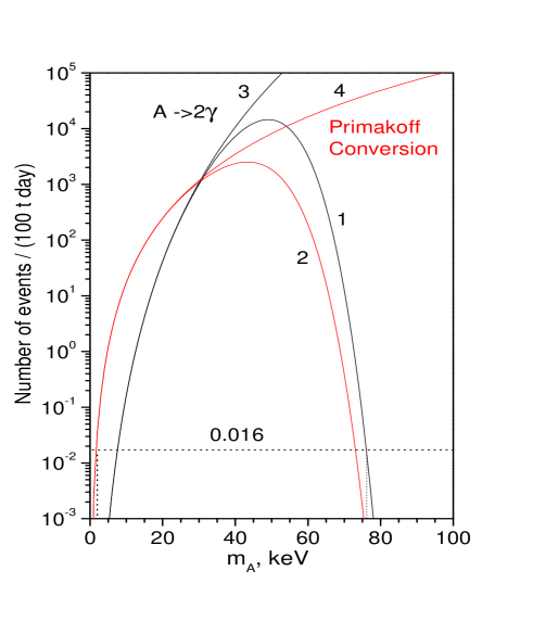
Figure 2: The expected number of axion decays (l) and inverse Primakoff conversions on ${}^{12}\rm{C}$ nuclei (2) in the 100 t per day for KSVZ axion model. Lines (3) and (4) show the corresponding curves under the assumption that axions do not decay during their flight from the Sun.

III.3 Escape of axions from the Sun

Axions could be captured within the Sun. The requirement that most axions escape the Sun thus limits the axion coupling strengths accessible to terrestrial experiments. Each of the 4 axion-matter interactions considered in this paper contribute to these limits.

The flux of 5.5 MeV axions on the Earth’s surface is proportional to the $pp$-neutrino flux, as given in equation (7), only when the axion lifetime exceeds the time of flight from the Sun and when the flux is not reduced as a result of axion absorption by solar matter. Axions produced at the center of the Sun cross a layer of approximately $6.8\times 10^{35}$ electrons/${\rm{cm}}^{2}$ in order to reach the Sun’s surface. Axion loss due to Compton conversion into photons in the solar matter imposes an upper limit on $g_{Ae}$ after which the sensitivity of terrestrial experiments using solar axions is reduced. The cross section of the Compton conversion reaction for 5.5-MeV axions depends weakly on the axion mass and can be written as $\sigma_{CC}\approx g^{2}_{Ae}\times 4.3\times 10^{-25}{\rm{cm}}^{2}$. For $g_{Ae}$ values below $10^{-6}$, the axion flux is not substantially suppressed.

The maximum cross section of the axio-electric effect on atoms is $\sigma_{Ae}\approx g^{2}_{Ae}Z^{2}1.9\times 10^{-29}{\rm{cm}}^{2}$ (see Fig.1 for carbon). The abundance of heavy ($Z>50$) elements in the Sun is $\sim 10^{-9}$ in relation to hydrogen Asp06 . If $g_{Ae}<10^{-3}$, the change in the axion flux does not exceed 10%.

The axion-photon interaction, as determined by the constant $g_{A\gamma}$, leads to the conversion of an axion into a photon in a field of nucleus. The cross section of the reaction is $\sigma_{pc}\approx g^{2}_{A\gamma}Z^{2}\times 1.8\times 10^{-29}{\rm{cm}}^{2}$. Taking into account the density of ${}^{1}\rm{H}$ and ${}^{4}\rm{He}$ nuclei, the condition that axions efficiently escape the Sun imposes the constraint $g_{A\gamma}<10^{-4}{\rm{GeV}}^{-1}$. Constraint for the other elements are negligible due to their low concentration in the Sun.

The axion-nucleon interaction leads to axion absorption in a threshold reaction similar to photo–dissociation: $A+Z\rightarrow Z_{1}+Z_{2}$. For axions with energy 5.5-MeV this can occur for only a few nuclei: ${}^{17}{\rm{O}}$,${}^{13}{\rm{C}}$, and ${}^{2}{\rm{H}}$. It was shown in Raf82 that axio–dissociation cannot substantially reduce the axion flux for $g_{AN}<10^{-3}$.

In all, the requirement that most axions escape the Sun sets these limits on the matter-axion couplings - $g_{Ae}<10^{-6}$, $g_{A\gamma}<10^{-4}{\rm{GeV}}^{-1}$ and $g_{AN}<10^{-3}$.

IV Experimental set-up and measurements

IV.1 Brief description of Borexino

Borexino is a real-time detector for solar neutrino spectroscopy located at the Gran Sasso Underground Laboratory. Its main goal is to measure low energy solar neutrinos via ($\nu$,e)-scattering in an ultra-pure liquid scintillator. At the same time, however, the extremely high radiopurity of the detector and its large mass allow it to be used to study other fundamental questions in particle physics and astrophysics.

The main features of the Borexino detector and its components have been thoroughly described in Ali02 -Bel12B . Borexino is a scintillator detector with an active mass of 278 tons of pseudocumene (C₉H₁₂), doped with 1.5 g/liter of PPO (C₁₅H₁₁NO). The scintillator is housed in a thin nylon vessel (inner vessel - IV) and is surrounded by two concentric pseudocumene buffers (323 and 567 tons) doped with a small amount of light quencher (dimethyl phthalate - DMP) to reduce their scintillation. The two buffers are separated by a second thin nylon membrane to prevent diffusion of radon coming from PMTs, light concentrators and SSS walls towards the scintillator. The scintillator and buffers are contained in a Stainless Steel Sphere (SSS) with diameter 13.7 m. The SSS is enclosed in an 18.0-m diameter, 16.9-m high domed Water Tank (WT), containing 2100 tons of ultra pure water as an additional shield against external $\gamma$’s and neutrons. The scintillation light is detected by 2212 8” PMTs uniformly distributed on the inner surface of the SSS. The WT is equipped with 208 additional PMTs that act as a Cerenkov muon detector (outer detector) to identify the residual muons crossing the detector. All the internal components of the detector were selected following stringent radiopurity criteria.

IV.2 Detector calibration. Energy and spatial resolutions.

In Borexino, charged particles are detected by scintillation light induced by their interactions with the liquid scintillator. The energy of an event is related to the total collected light by the PMTs. In a simple approach, the response of the detector is assumed to be linear with respect to the energy released in the scintillator. The coefficient linking the event energy and the total collected charge is called the light yield (or photo-electron yield). Deviations from linearity at low energies can be taken into account including the ionization deficit function $f(k_{B},E)$, where $k_{B}$ is the empirical Birks’ constant.

The detector energy and spatial resolution were studied with radioactive sources placed at different positions inside the inner vessel. For relatively high energies ( $>$2 MeV), which are of interest for 5.5 MeV axion studies, the energy calibration was performed with a ²⁴¹Am-⁹Be neutron source. One can find a detailed description of the energy calibration in Bel10 ; Bel10A . Deviations of the $\gamma$-peak positions from linearity was less than 30 keV over the whole energy range. The energy resolution scales approximately as ${(\sigma/E)}$ $\simeq(0.058+1.1\times 10^{-3}E)/\sqrt{E}$ where E is given in MeV units. The position of an event is determined using a photon time of flight reconstruction algorithm. The resolution of the event reconstruction, as measured using the ²¹⁴Bi-²¹⁴Po $\beta-\alpha$ decay sequence, is 13$\pm$2 cm Ali09 .

IV.3 Data selection

The experimental energy spectrum from Borexino in the range (1.0-15) MeV, containing 737.8 live-days of data, is shown in Fig.3. At energies below 3 MeV, the spectrum is dominated by 2.6 MeV $\gamma$’s from the $\beta$-decay of ²⁰⁸Tl in the PMTs and in the SSS.

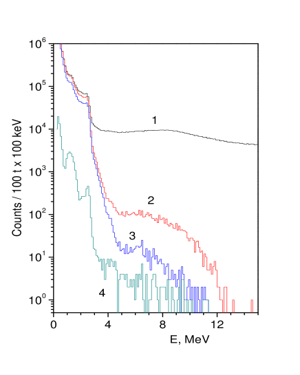
Figure 3: Energy spectra of the events and effect of the selection cuts. From top to bottom: (1) raw spectrum; (2) with 2 ms muon veto cut; (3) with events within 6.5 s of a muon crossing the SSS removed; (4) events inside FV

The spectrum obtained by vetoing all muons and events within 2 ms after each muon is shown by curve 2, Fig.3. Muons are rejected by the outer detector and by an additional cut on the mean time of the hits belonging to the cluster and on the time corresponding to the maximum density of hits. This cut rejects residual muons that were not tagged by the outer water Cherenkov detector and that interacted in the pseudocumene buffer regions (see Bel11B for more details).

To reduce the background due to short-lived isotopes (1.1 s ${}^{8}\rm{B}$, 1.2 s ${}^{8}\rm{Li}$, etc; see Bel10A ) induced by muons, an additional 6.5 s veto is applied after each muon crossing the SSS (curve 3, Fig.3). This cut induces 202.2 days of dead time that reduces the live-time to 535.6 days.

In order to reject external background in the 5.5 MeV energy region a fiducial volume cut is applied. Curve 4 of Fig.3 shows the effect of selecting a 100 ton fiducial volume (FV) by applying a cut R $\leq$ 3.02 m. Additionally, a pulse shape-discrimination analysis based on the Gatti optimal filter Gat62 is performed: events with negative Gatti variable corresponding to $\gamma$- and $\beta$-like signals are selected (see Ali09 for more details). This cut does not change the spectrum for energies higher than 4 MeV.

IV.4 Simulation of the Borexino response functions

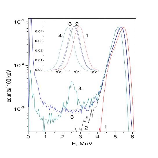
Figure 4: Simulated responses to axion interactions in the Borexino IV: 1- axio-electric effect ( 5.49 MeV electrons), 2- Compton axion to photon conversion (electrons and $\gamma$-quanta), 3- Primakoff conversion (5.49 MeV $\gamma$-quanta), 4- decay $A\rightarrow 2\gamma$. The inset shows the corresponding responses for events reconstructed within the FV.

The Monte Carlo (MC) method has been used to simulate the Borexino response $S(E)$ to electrons and $\gamma$-quanta produced by axion interactions. The MC simulations are based on the GEANT4 code, taking into account the effect of ionization quenching and non-linearity induced by the energy dependence on the event position. Uniformly distributed $\gamma$’s were simulated inside the entire inner vessel, but only those which reconstructed within the FV were used in determining the response function. The MC candidate events were selected by the same cuts applied in the real data selection.

The energy spectra of electrons and gammas from the axion Compton conversion were generated according to the differential cross section given in Don78 , Avi88 , Zhi79 for different axion masses Bel08 . The responses for the axion decay into two $\gamma$ quanta were calculated taking into account the angular correlation between photons. The response functions for axion Compton conversion (electron and $\gamma$-quanta with total energy of 5.5 MeV), for the axio-electric effect (electron with energy 5.5 MeV), axion decay (two $\gamma$-quanta with energy 2.75 MeV in case of non-relativistic axions) and for Primakoff conversion (5.5 MeV $\gamma$-quanta) are shown in Fig.4. The response functions are normalized to 1 axion interaction (decay) in the IV. The shift in the position of the total absorption peak for interactions involving $\gamma$’s is caused by an ionization quenching effect. All response functions are fitted with Gaussians.

V Results and discussions

V.1 Fitting procedure

Figure 5 shows the observed Borexino energy spectrum in the ($3.0-8.5$) MeV range in which the axion peaks might appear. The spectrum is modeled with a sum of exponential and Gaussian functions,

$$N^{\rm th}(E)=a+b\times e^{-cE}+(S/\sqrt{2\pi}\sigma)\times e^{-\frac{(E_{MC}-E)^{2}}{2\sigma^{2}}},$$ (20)

where the position $E_{MC}$ ($\cong$5.49 MeV) and dispersion $\sigma$ ($\cong$0.15 MeV) are taken from the MC response, $S$ is the peak intensity and $a,b$ and $c$ are the parameters of the function describing the continuous background.

The number of events in the axion peak $S$ was calculated using the maximum likelihood method. The likelihood function assumes the form of a product of Poisson probabilities:

$$L=\prod e^{-N^{\rm th}_{i}}({N^{\rm th}_{i}})^{N^{\rm exp}_{i}}/N^{\rm exp}_{i}!$$ (21)

where $N^{\rm th}_{i}$ and $N^{\rm exp}_{i}$ are the expected (20) and measured number of counts in the i-th bin of the spectrum, respectively. The dispersion of the peak ($\sigma$) was fixed, while the position ($E_{0}$) was varied around $E_{MC}\pm 30$ keV, to take into account the uncertainty in the energy scale. The others 4 parameters ($a,b,c$ and $S$) were also free. The total number of the degrees of freedom in the range of 3.2 -8.4 MeV was 46.

The fit results, corresponding to the maximum of $L$ at $S$=0 are shown in Fig.5. The value of modified $\chi^{2}=\sum(N^{\rm exp}_{i}-N^{\rm th}_{i})^{2}/N^{\rm th}_{i}$ is $\chi^{2}$= 44/46. Because of the low statistics, a Monte Carlo simulation of (20) is used to find the probability of $\chi^{2}_{p}\geq$ 44. The goodness-of-fit ($p=52\%$) shows that the background is well described by function (20). The upper limit on the number of counts in the peak was found using the $L_{\rm{max}}(S)$ profile, where $L_{\rm{max}}(S)$ is the maximal value of $L$ for fixed $S$ while all others parameters were free. The distribution of $L_{\rm{max}}(S)$ values obtained from the MC simulations for $S\geq 0$ was used to determine confidence levels in $L_{\rm max}(S)$. The limits obtained on the number of events for different processes are shown in table 1.

Table 1: The upper limits on the number of axions registered in Borexino FV (counts/536 days). CC - Compton axion to photon conversion, $A+e\rightarrow e+\gamma$; AE - axio-electric effect, $A+e+Z\rightarrow e+Z$; PC - Primakoff conversion on nuclei, $A+^{12}C\rightarrow\gamma+^{12}C$. The limits are given at 68(90)$\%$ c.l.

reaction	CC	AE	$A$$\rightarrow$2$\gamma$	PC
$S^{\rm lim}$	3.8 (6.9)	3.4 (6.5)	4.8 (8.4)	3.8 (6.9)

The limits obtained ($S^{\rm lim}_{CC}\simeq$ 0.013 c/(100 t day) at 90% c.l.) are very low, e.g. $\sim 10^{4}$ times lower than expected number of events from $pp-$ neutrino (135 c/(100 t day)). The upper limits on the number of events with energy 5.5 MeV constrain the product of axion flux $\Phi_{A}$ and the interaction cross section with electron, proton or carbon nucleus $\sigma_{A-e,p,C}$ via

$$S_{\rm events}=\Phi_{A}\sigma_{A-e,p,C}N_{e,p,C}T\varepsilon\leq S^{\rm lim},$$ (22)

where $N_{e,p,C}$ is the number of electrons, protons and carbon nuclei in the IV, T is the measurement time and $\varepsilon$ is the detection efficiency. The individual rate limits are:

$$\Phi_{A}\sigma_{A-e}\leq 4.5\times 10^{-39}\rm{s^{-1}}$$ (23)

$$\Phi_{A}\sigma_{A-p}\leq 2.5\times 10^{-38}\rm{s^{-1}}$$ (24)

$$\Phi_{A}\sigma_{A-C}\leq 3.3\times 10^{-38}\rm{s^{-1}}.$$ (25)

These limits show very high sensitivity to a model-independent value $\Phi_{A}\sigma_{A}$. For comparison the standard solar neutrino capture rate is SNU = $10^{-36}\rm{s^{-1}}\rm{atom^{-1}}$. A capture rate of solar neutrinos measured by Ga-Ge radiochemical detectors is about 70 SNU.

V.2 Limits on $g_{Ae}$ and $g_{AN}$ couplings

The number of expected events due to Compton conversion in the FV of the detector are:

$$S_{CC}=\Phi_{\nu pp}(\omega_{A}/\omega_{\gamma})\sigma_{CC}N_{e}T\varepsilon$$ (26)

where $\sigma_{CC}$ is the Compton conversion cross sections, $\Phi_{A}=\Phi_{\nu pp}(\omega_{A}/\omega_{\gamma})$ is the axion flux (7), $N_{e}=9.17\times 10^{31}$ is the number of electrons in the IV; $T=4.63\times 10^{7}$ s is the exposure time; and $\varepsilon=0.358$ is the detection efficiency obtained with MC simulations (Fig.4).

The axion flux $\Phi_{A}$ is proportional to the constant $(g_{3AN})^{2}$, and the cross section $\sigma_{CC}$ is proportional to the constant $g^{2}_{Ae}$, according to expressions (7) and (8). The $S_{CC}$ value depends, then, on the product of the axion-electron and axion-nucleon coupling constants: $g^{2}_{Ae}\times(g_{3AN})^{2}$. According to Eqs. (7) and (10), and taking into account the approximate equality of the momenta of the axion and the $\gamma$-quantum ($(p_{A}/p_{\gamma})^{3}\simeq 1$ for $m_{A}\leq 1$ MeV), the expected number of events can be written as:

$$S_{CC}=g^{2}_{Ae}\times g^{2}_{3AN}\times 1.4\times 10^{-14}N_{e}T\varepsilon=$$

$$=g^{2}_{Ae}\times g^{2}_{3AN}\times 2.1\times 10^{25}.$$ (27)

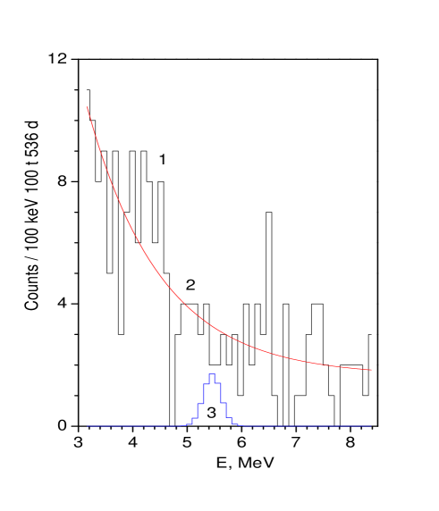
Figure 5: The fitted Borexino spectrum in the ($3.2-8.4$) MeV range. Curve 3 is the detector response function for Compton axion-photon conversion at the 90% c.l. upper limit ($S$=6.9 events).

Using this relationship, the experimental $S_{CC}^{\rm lim}$ can be used to constrain $g_{Ae}\times g_{3AN}$ and $m_{A}$. The range of excluded $|g_{Ae}\times g_{3AN}|$ values is shown in Fig.6 (line 2). At $(p_{A}/p_{\gamma})^{3}\approx 1$ or $m_{A}<1\rm{MeV}$ the limit is:

$$|g_{Ae}\times g_{3AN}|\leq 5.5\times 10^{-13}~{}\rm{(90\%~{}c.l.).}$$ (28)

The dependence of $|g_{Ae}\times g_{3AN}|$ on $m_{A}$ arises from the kinematic factor in equations (6) and (8); thus,these constraints are completely model-independent and valid for any pseudoscalar particle. It’s important to stress that the limits were obtained on the assumption that axions escape from the Sun and reach the Earth, which implies $g_{Ae}<10^{-6}$ for $m_{A}<2m$ and $g_{Ae}<(10^{-11}-10^{-12})$ if $m_{A}>2m$ (Der10 ).

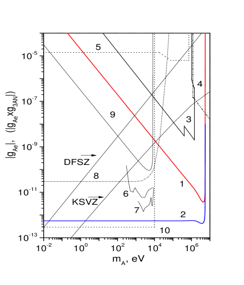
Figure 6: The limits on the $g_{Ae}$ coupling constant obtained by 1- present work, 2 - present work for $|g_{Ae}\times g_{3AN}|$, 3- reactor Alt95 ; Cha07 and solar experiments Bel08 ; Der10 , 4- beam dump experiments Kon86 ; Bjo88 , 5- ortho-positronium decay Asa91 , 6- CoGeNT Aal08 , 7- CDMS Ahm09 , 8- solar axion luminosity Gon09 , 9-resonance absorption Der11 , 10- read giant Raf08 . The excluded values are located above the corresponding lines. The relations between $g_{Ae}$ and $m_{A}$ for KSVZ- and DFSZ-models are shown also.

Within the hadronic (KSVZ) axion model, $g_{3AN}$ and $m_{A}$ are related by expression (II), which can be used to obtain a constraint on the $g_{Ae}$ constant, depending on the axion mass (Fig.6. line 1). For $(p_{A}/p_{\gamma})^{3}\approx 1$ the limit on $g_{Ae}$ and $m_{A}$ is:

$$|g_{Ae}\times m_{A}|\leq 2.0\times 10^{-5}\rm{~{}eV}~{}\rm{(90\%~{}c.l.),}$$ (29)

where $m_{A}$ is given in eV units. For $m_{A}$ = 1 MeV, this constraint corresponds to $g_{Ae}\leq 2.0\times 10^{-11}$. Figure 6 shows the constraints on $g_{Ae}$ that were obtained in experiments with reactor, accelerator, and solar axions, as well as constraints from astrophysical arguments.

V.3 Limits on $g_{A\gamma}$ and $g_{AN}$ couplings

The analysis of $A\rightarrow 2\gamma$ decay and Primakoff photoproduction is more complicated because axions can decay during their flight from the Sun. The exponential dependence of the axion flux on $g_{a\gamma}$ and $m_{A}$, given by (17), must be taken into account.

The number of events detected in the FV due to axion decays into 2 $\gamma$’s within the IV are:

$$S_{2\gamma}=N_{\gamma}T\varepsilon_{2\gamma}$$ (30)

where $N_{\gamma}$ is given by (18) and $\varepsilon_{2\gamma}$ = 0.35 is the detection efficiency obtained by MC simulation. The relation $S_{2\gamma}<S^{\rm lim}_{A\rightarrow 2\gamma}$ leads to model-independent limits on $g_{3AN}^{2}\times g_{A\gamma}^{2}$ vs axion mass. The expected value of $S_{2\gamma}$ has a complex dependence on $g_{A\gamma}$, $g_{3AN}$ and $m_{A}$ given by equations (14)-(18).

In the assumption that $\beta\approx 1$ the number of decays in the FV depends on $g_{3AN}^{2}$, $g_{A\gamma}^{2}$ and $m_{A}^{4}$:

$$N_{\gamma}=1.68\times 10^{-4}g^{2}_{A\gamma}\times g_{3AN}^{2}\times m_{A}^{4},$$ (31)

where $g_{A\gamma}$ and $m_{A}$ are given in $\rm{GeV}^{-1}$ and eV units, respectively. The limit derived from equation (30), at 90% c.l., is

$$|g_{A\gamma}\times g_{3AN}|\times m_{A}^{2}\leq 3.3\times 10^{-11}\rm{~{}eV}.$$ (32)

The dependence of $S_{2\gamma}$ on $g_{A\gamma}$ and $m_{A}$ is obtained from (II), which gives the relationship between $g_{3AN}$ and $m_{A}$ in the KSVZ model. The relation $S_{2\gamma}\leq S^{\rm lim}_{A\rightarrow 2\gamma}$ imposes constraints on the range of $g_{A\gamma}$ and $m_{A}$ values. The excluded region is inside contour 1a in Fig.7 (90 % c.l.). For higher values of $g_{A\gamma}^{2}m_{A}^{3}$ axions decay before they reach the detector, while for lower $g_{A\gamma}^{2}m_{A}^{3}$ the probability of axion decay inside the Borexino volume is too low. The limits on $g_{A\gamma}$ obtained by other experiments are also shown.

The Borexino results exclude a large new region of axion-photon coupling constant $(2\times 10^{-14}-10^{-7})\rm{GeV}^{-1}$ for the axion mass range $(0.01-5)$ MeV. The Borexino limits are about 2-4 order of magnitude stronger than those obtained by laboratory-based experiments using nuclear reactors and accelerators. Moreover, our excluded region has begun to overlap the predicted regions from heavy axion models Bere00 ; Bere01 ; Hal04 .

At $m_{A}<1\rm{MeV}$ the constraint on $g_{A\gamma}$ and $m_{A}$ is given by

$$|g_{A\gamma}|\times m_{A}^{3}\leq 1.2\times 10^{-3}\rm{~{}eV^{2}}.$$ (33)

So, e.g., $m_{A}$=1 MeV corresponds to $g_{A\gamma}\leq 1.2\times 10^{-12}\rm{~{}GeV^{-1}}$. Under the assumption that the axion-photon coupling $g_{A\gamma}$ depends on axion mass as in the KSVZ model (15), we exclude axions with mass in the (7.5 - 76) keV range (see Fig.2). Similar constraints can be obtained for DFSZ axions for specific values of $\cos^{2}\beta_{\rm{dfsz}}$.

The number of expected events due to inverse Primakoff conversion is:

$$S_{PC}=\Phi_{A}\sigma_{PC}N_{C}T\varepsilon_{PC}$$ (34)

where $\sigma_{PC}$ is the Primakoff conversion cross sections; $N_{C}$ is the number of carbon nuclei in the IV, and $\varepsilon_{PC}$ is the detection efficiency for 5.5 MeV $\gamma$’s. The axion flux, $\Phi_{A}$, is proportional to the constant $g^{2}_{3AN}$, and the cross section $\sigma_{PC}$ is proportional to the constant $g^{2}_{A\gamma}$, according to equations (7) and (19). As a result, the $S_{PC}$ value depends on the product of the axion-photon and axion-nucleon coupling constants: $g^{2}_{A\gamma}\times g^{2}_{3AN}$. Under the assumption that $\Phi_{A}\approx\Phi_{A0}$ (true for $g_{A\gamma}(\rm{GeV^{-1}})\times m_{A}^{2}\rm{(eV)}<1.2\times 10^{4}$) one can obtain the limit:

$$|g_{A\gamma}\times g_{3AN}|\leq 4.6\times 10^{-11}\rm{~{}GeV^{-1}}~{}{\rm(90\%~{}c.l.),}$$ (35)

where again $g_{A\gamma}$ is in GeV^-1 units. This limit is 25 times stronger than the one obtained by CAST And10 , which searches for conversion of 5.5 MeV axions in a laboratory magnetic field ($|g_{A\gamma}\times g_{3AN}|\leq 1.1\times 10^{-9}$ at $m_{A}\leq 1\rm{eV}$).

In the KSVZ model (II), the constraint on $g_{A\gamma}$ and $m_{A}$ is given by the relation:

$$|g_{A\gamma}|\times m_{A}\leq 1.7\times 10^{-12}.$$ (36)

For $m_{A}$=1 MeV, this corresponds to $g_{A\gamma}\leq 1.7\times 10^{-9}\rm{~{}GeV^{-1}}$. The region of excluded values of $g_{A\gamma}$ and $m_{A}$ are shown in Fig.7, line 1b; under the assumption that $g_{A\gamma}$ depends on $m_{A}$ as in the KSVZ model (15) we exclude axions with masses between (1.5 - 73) keV (see Fig.2). Our results from the inverse Primakoff process exclude a new region of $g_{A\gamma}$ values at $m_{A}\sim$ 10 keV.

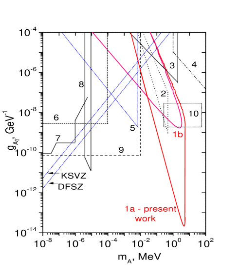
Figure 7: The limits on $g_{A\gamma}$ obtained by 1- present work (a - $A\rightarrow 2\gamma$, b - PC, areas of excluded values are located inside contour), 2 - CTF Bel08 , 3- reactor experiment Cha07 , 4- beam dump experiments Kon86 ; Bjo88 , 5- resonant absorption Der09 , 6- solar axions conversion in crystals - Avi99 ; Ber01 ; Mor02 , 7- CAST and Tokyo helioscope Zio05 ; Ari09 ; Ino08 , 8-telescopes Ber91 ; Res91 ; Gri07 , 9- HB Stars Raf08 , 10- expectation region from heavy axion models Bere00 ; Bere01 ; Hal04 .

VI CONCLUSIONS

A search for 5.5 MeV solar axions emitted in the $p(d,\rm{{}^{3}He})A$ reaction has been performed with the Borexino detector. The Compton conversion of axions into photons, the decay of axions into two photons, and inverse Primakoff conversion on nuclei were studied. The signature of all these reactions is a 5.5 MeV peak in the energy spectrum of Borexino. No statistically significant indications of axion interactions were found. New, model independent, upper limits on the axion coupling constants to electrons, photons and nucleons,

$$|g_{Ae}\times g_{3AN}|\leq 5.5\times 10^{-13}$$ (37)

and

$$|g_{A\gamma}\times g_{3AN}|\leq 4.6\times 10^{-11}\rm{GeV^{-1}},$$ (38)

were obtained at $m_{A}<1\rm{MeV}$ and 90% c.l.

Under the assumption that $g_{3AN}$ depends on $m_{A}$ as in the KSVZ axion model, new 90% c.l. limits on axion-electron and axion-photon coupling as a function of axion mass were obtained:

$$|g_{Ae}\times m_{A}|\leq 2.0\times 10^{-5}\rm{~{}eV}$$ (39)

and

$$|g_{A\gamma}\times m_{A}|\leq 1.7\times 10^{-12}.$$ (40)

The new Borexino results exclude large regions of axion-electron and axion-photon coupling constants ($g_{Ae}\in(10^{-11}-10^{-9})$ and $g_{A\gamma}\in(2\times 10^{-14}-10^{-7})\rm{GeV}^{-1}$) for the axion mass range $(0.01-5)$ MeV.

VII ACKNOWLEDGMENTS

The Borexino program was made possible by funding from INFN and PRIN 2007 MIUR (Italy), NSF (USA), BMBF, DFG, and MPG (Germany), NRC Kurchatov Institute (Russia), and MNiSW (Poland). We acknowledge the generous support of the Laboratori Nazionali del Gran Sasso (LNGS). A. Derbin, L. Ludhova and O. Smirnov acknowledge the support of Fondazione Cariplo.

References

- (1) S. Weinberg, Phys. Rev. Lett. 40, 223 (1978).
- (2) F. Wilczek, Phys. Rev. Lett. 40, 279 (1978).
- (3) R.D. Peccei and H.R. Quinn, Phys. Rev. Lett. 38, 1440 (1977).
- (4) K. Nakamura et al., (Particle Data Group), J. Phys. G37, 075021 (2010).
- (5) J.E. Kim, Phys. Rev. Lett. 43, 103 (1979).
- (6) M.A. Shifman, A.I. Vainstein, and V.I. Zakharov, Nucl. Phys. B166, 493 (1980).
- (7) A.R. Zhitnitskii, Yad. Fiz. 31, 497 (1980) [Sov. J. Nucl. Phys. 31, 260 (1980).
- (8) M. Dine, F. Fischler and M. Srednicki, Phys. Lett. B104, 199 (1981).
- (9) D.B. Kaplan, Nucl. Phys. B260, 215 (1985).
- (10) Z. Berezhiani and A. Drago, Phys. Lett. B473, 281 (2000).
- (11) Z. Berezhiani, L. Gianfanga, and M. Giannotti, Phys. Lett. B500, 286 (2001).
- (12) L.J. Hall and T. Watari, Phys. Rev. D70, 115001 (2004).
- (13) A.M. Serenelli, W.C. Haxton and C. Peña-Garay, arXiv:1104.1639.
- (14) G. Bellini et al. (Borexino Coll.), Phys. Rev. Lett. 107, 141302 (2011).
- (15) G. Bellini et al., (Borexino coll.) Europ. Phys. J. C54, 61 (2008).
- (16) W.C. Haxton and K.Y. Lee, Phys. Rev. Lett. 66, 2557 (1991).
- (17) T.W. Donnelly et al., Phys. Rev. D18, 1607 (1978).
- (18) F.T. Avignone III et al., Phys. Rev. D37, 618 (1988).
- (19) M. Srednicki, Nucl. Phys. B260, 689 (1985).
- (20) V. Mateu and A. Pich, J. High Energy Phys. 10, 41 (2005).
- (21) G. Altarelli et al., Phys. Lett. B46, 337 (1997).
- (22) D. Adams et al., Phys. Rev. D56, 5330 (1997).
- (23) G.J. Schmid et al., Phys. Rev. C56, 2565 (1997).
- (24) A.R. Zhitnitskii and Yu.I. Skovpen , Yad. Fiz. 29, 995 (1979).
- (25) A.V. Derbin, A.S. Kayunov, and V.N. Muratova, Bull. Rus. Acad. Sci. Phys. 74, 805 (2010), arXiv:1007.3387
- (26) M. Asplund, N. Grevesse, and J. Sauval, Nucl. Phys. A777, 1 (2006).
- (27) G. Raffelt and L. Stodolsky, Phys. Lett. B119, 323 (1982).
- (28) G. Alimonti et al. (Borexino Coll.), Astropart. Phys. 16, 205 (2002)
- (29) C. Arpesella et al. (Borexino Coll.), Phys. Lett. B568, 101 (2008).
- (30) C. Arpesella et al. (Borexino Coll.), Phys. Rev. Lett. 101, 091302 (2008).
- (31) G. Alimonti et al. (Borexino Coll.), Nucl. Instr. and Meth. A600, 58 (2009).
- (32) G. Bellini et al. (Borexino Coll.), Phys. Rev. C81, 034317,(2010).
- (33) G. Bellini et al. (Borexino Coll.), Phys. Rev. D82, 033006,(2010).
- (34) G. Bellini et al. (Borexino Coll.), Phys. Lett. B696, 191 (2011).
- (35) G. Bellini et al. (Borexino Coll.), JINST, 6, P05005 (2011). arXiv:1101.3101
- (36) G. Bellini et al. (Borexino Coll.), Phys. Lett. B707 22 (2012). arXiv:1104.2150
- (37) G. Bellini et al. (Borexino Coll.), Phys. Rev. Lett. 108, 051302 (2012). arXiv:1110.3230
- (38) E. Gatti and F. De Martini, Nuclear Electronics, IAEA Wien, 2, 265 (1962).
- (39) M. Altmann et al., Z. Phys. C68, 221 (1995).
- (40) H.M. Chang et al. (Texono Coll.), Phys. Rev. D75, 052004 (2007).
- (41) A. Konaka et al., Phys. Rev. Lett. 57, 659 (1986).
- (42) J.D. Bjorken et al., Phys. Rev. D38, 3375 (1988).
- (43) S. Asai et al., Phys. Rev. Lett. 66, 2440 (1991).
- (44) C.E. Aalseth et al.,(CoGeNT Coll.), Phys. Rev. Lett. 101, 251301 (2008).
- (45) Z. Ahmed et al., (CDMS Coll.), Phys. Rev. Lett. 103, 141802 (2009).
- (46) A.V. Derbin et al., Phys. Rev. D83, 023505 (2011).
- (47) P. Gondolo and G.G. Raffelt, Phys. Rev. D79, 107301 (2009).
- (48) G.G. Raffelt, Lect. Notes Phys. 741, 51 (2008).
- (49) A.V. Derbin et al., Phys. Lett. B678, 181 (2009).
- (50) F.T. Avignone et al., (Solax Coll.), Nucl. Phys., (Proc. Supl.) 72, 176 (1999).
- (51) R. Bernabei et al., (DAMA Coll), Phys. Lett. B515, 6 (2001).
- (52) A. Morales et al., (Cosme Coll.), Astropart. Phys. 16, 325 (2002).
- (53) K. Zioutas et al., (CAST Coll.), Phys. Rev. Lett. 94, 121301 (2005).
- (54) E. Arik et al., (CAST Coll.), JCAP0902, 008 (2009). arXiv:0810.4482
- (55) Y. Inoue et al., Phys. Lett. B668, 93 (2008).
- (56) M.B. Bershady, M.D. Ressell, and M.S. Turner, Phys. Rev. Lett. 66, 1398 (1991).
- (57) M.D. Ressell, Phys. Rev. D66, 3001 (1991).
- (58) D. Grin et al., Phys. Rev. D75, 105018 (2007).
- (59) S. Andriamonje et al., (CAST Coll.), JCAP 1003:032 (2010). arXiv:0904.2103