A relationship between two graphical models of the Kauffman polynomial

Abstract

There are two oriented 4-valent graphical models for the Kauffman polynomial: one ($HJ$) is obtained by combining Jaeger’s formula and Kauffman-Vogel model for the Homflypt polynomial; the other ($WF$) is obtained by combining Kauffman-Vogel model for the Kauffman polynomial and Wu’s formula. The main goal of this paper is to explore the relationship between the two models. We find that there is an one-to-many correspondence between the terms of $HJ$ model and the terms of $WF$ model. In addition, we investigate the relation between trivalent graphical models and 4-valent graphical models of both the Homflypt and Kauffman polynomials, and observe that there is a bijection between the terms of the two models.

Keywords: Kauffman polynomial, 4-valent graph, Jaeger’s formula, Homflypt polynomial, Trivalent graph, Relationship.

MSC: 57M25 57M15

1 Introduction

In [16, 19], Kauffman and Vogel generalized the Homflypt and Kauffman polynomials from links to 4-valent rigid vertex spatial graphs. Conversely, an unoriented (resp. oriented) 4-valent plane graph expansion for the Kauffman (resp. Homflypt) polynomial of unoriented (resp. oriented) links was obtained, which is implicit in [19]. In 1989, Jaeger announced a relation [18], we shall call it Jaeger’s formula, between the Kauffman polynomial of an unoriented link diagram and the Homflypt polynomials of some oriented link diagrams constructed from the unoriented link diagram. Recently, Wu generalized Jaeger’s formula from link diagrams to 4-valent rigid vertex spatial graph diagrams [25]. We shall call it Wu’s formula. Note that 4-valent rigid vertex spatial graph diagrams include 4-valent plane graphs as a special case. In this paper we shall confine ourselves in 4-valent plane graphs.

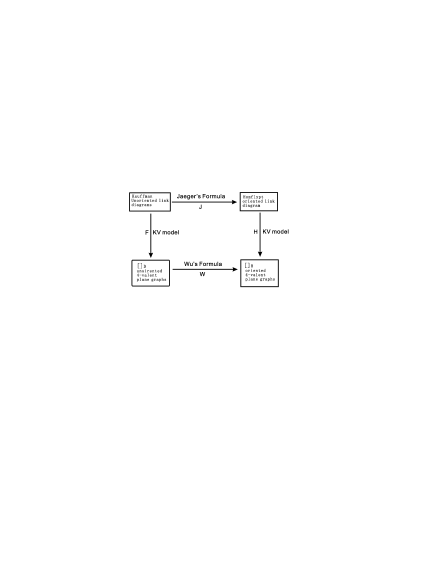
Fig. 1: The relation diagram.

We illustrate above descriptions by a relation diagram as shown in Fig. 1. According to the diagram, two oriented 4-valent graphical models for the Kauffman polynomial will be produced: one ($HJ$) is obtained by combining Jaeger’s formula and Kauffman-Vogel model for the Homflypt polynomial; the other ($WF$) is obtained by combining Kauffman-Vogel model for the Kauffman polynomial and Wu’s formula. The first and main goal of this paper is to explore the relationship between the two models. We modify the Jaeger’s formula and then find that there is an one-to-many correspondence between the terms of $HJ$ model and the terms of $WF$ model.

As a result, we actually verified the consistency of the two Kauffman-Vogel models, Jaeger’s formula and Wu’s formula. We pointed that in [11], Huggett found and verified a relationship (i.e. the replacement of a crossing by a clasp) between a famous Thistlethwaite’s result [23] which expresses the Jones polynomial as a special parametrization of the Tutte polynomial [24] and a Jaeger’s result relating the Homflypt polynomial with the Tutte polynomial.

Then we investigate the relation between trivalent graphical models [21, 8, 4] and 4-valent graphical models of both the Homflypt and Kauffman polynomials. We observed there is a bijection between the terms of the two models via contracting “thick” edges of trivalent plane graphs to obtain 4-valent plane graphs.

2 Homflypt and Kauffman polynomials

To proceed rigorously, it is necessary to recall the definition of the Homflypt and Kauffman polynomials. The Homflypt polynomial was introduced in [9] and [22], independently, which is a writhe-normalization of its regular isotopy counterpart: the $R$ polynomial. Let $L$ be an oriented link diagram. We denote by $R_{L}(z,a)\in\mathbf{Z}[z^{\pm},a^{\pm}]$ the $R$ polynomial of $L$.

Axioms for the $R$ polynomial

1. $R_{\circlearrowright}=1$.

2. $R_{L}$ is invariant under Reidemeister moves II and III.

3. (the kink formulae) The effect of Reidemeister move I on $R$ is to multiply by $a$ or $a^{-1}$ according to the type of Reidemeister move I:

   $$R_{L(+)}=aR_{L},\ \ R_{L(-)}=a^{-1}R_{L},$$ (1)

   where $L(+)$ (resp. $L(-)$ denotes diagrams with a positive (resp. negative) curl and $L$ denotes the result of removing this curl by Reidemeister move I.

4. (the skein relation)

   $$R_{L_{+}}-R_{L_{-}}=zR_{L_{0}},$$ (2)

   where $L_{+},L_{-}$ and $L_{0}$ are link diagrams which are identical except near one crossing where they are as in Fig. 2 and are called a skein triple.

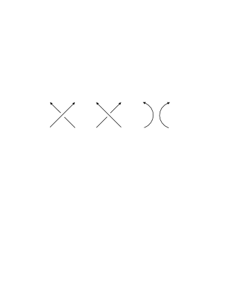
Fig. 2: A skein triple: $L_{+}$, $L_{-}$ and $L_{0}$.

The Alexander-Conway [1, 6] and Jones [13] polynomials are both special cases of the Homflypt polynomial.

The Kauffman polynomial was introduced in [17]. We work with its “Dubrovnik” version [20]. Let $L$ be an unoriented link diagram. We denote by $D_{L}(z,a)\in\mathbf{Z}[z^{\pm},a^{\pm}]$ the Dubrovnik (briefly, $D$) polynomial of $L$. The Dubrovnik polynomial satisfies the following axioms:

Axioms for the $D$ polynomial

1. $D_{\bigcirc}=1$.

2. $D_{L}$ is invariant under Reidemeister moves II and III.

3. (the kink formulae) The effect of Reidemeister move I on $D$ is to multiply by $a$ or $a^{-1}$ according to the type of Reidemeister move I:

   $$D_{L(+)}=aD_{L},\ \ D_{L(-)}=a^{-1}D_{L},$$ (3)

   where $L(+)$ (resp. $L(-)$ denotes diagrams with a positive (resp. negative) curl and $L$ denotes the result of removing this curl by Reidemeister move I.

4. (the switching formula)

   $$D_{L_{+}}-D_{L_{-}}=z(D_{L_{0}}-D_{L_{\infty}}),$$ (4)

   where $L_{+},L_{-},L_{0}$ and $L_{\infty}$ are link diagrams which are identical except near one crossing where they are as shown in Fig. 3.

Fig. 3: The quadruple: $L_{+}$, $L_{-}$, $L_{0}$ and $L_{\infty}$ (from left to right).

The Kauffman polynomial is a writhe-normalization of the Dubrovnik polynomial, which is the generalization of both the Jones polynomial [13] and the BLM-Ho’s $Q$ polynomial [3, 10]. The $D$ polynomial specializes to the Kauffman bracket polynomial [14] by putting $a=-A^{3}$ and $z=A-A^{-1}$ [18].

We point out that, when we mention the Homflypt and Kauffman polynomials we sometime mean the $R$ and $D$ polynomials, respectively.

3 Kauffman-Vogel models

In this section, we explain the 4-valent graphical models of the $R$ and $D$ polynomials. A graph is planar if it can be embedded in the plane, that is, it can be drawn on the plane so that no two edges intersect. The embedding of a planar graph is called a plane graph. It is well known that any graph can be embedded in the 3-dimensional Euclidean space [2], and such an embedding is called a spatial graph.

A 4-valent graph is a graph whose each vertex is of degree 4. We always consider simple closed curves called free loops as special cases of 4-valent graphs, in other words, a free loop is a graph having one edge and having no vertices.

In [16], Kauffman defined 4-valent graphs with rigid vertices and introduced the notion of rigid vertex ambient isotopy for 4-valent rigid vertex spatial graphs. In [19], Kauffman and Vogel introduced two 3-variable ($A,B,a$) polynomials for 4-valent rigid vertex spatial graphs in terms of the $R$ and $D$ polynomials, respectively. When $G$ has no vertices, i.e. $G$ is a link, The two 3-variable polynomials of 4-valent rigid vertex spatial graph $G$ will specialize to $R$ and $D$ polynomials, respectively.

Conversely, the $R$ and $D$ polynomials of link diagrams can be expressed as the sum of such 3-variable polynomials of 4-valent plane graphs constructed from link diagrams. In [5], Carpentier proved that such 3-variable polynomials can be computed recursively completely within the category of planar graphs without resorting to links. Thus we obtain 4-valent plane graphical models for both the $R$ and $D$ polynomials. Now we give a detailed account of the two models.

3.1 $R$ polynomial

By an oriented 4-valent plane graph, we mean a 4-valent plane graph together with an edge orientation of the graph such that at each vertex, the four (not necessarily distinct) edges incident with the vertex are oriented like a crossing of an oriented link diagram as shown in Fig. 4.

Fig. 4: Crossing-like oriented vertex.

The 3-variable polynomial $[G]_{R}=[G]_{R}(A,B,a)$ for an oriented 4-valent plane graph $G$ can be defined via the following graphical calculus [19].

Graphical calculus for the $[]_{R}$ polynomial

1. $[\circlearrowright]_{R}=1$, where $\circlearrowright$ is a free loop and its orientation is actually irrelevant.

2. $[G\sqcup\circlearrowright]_{R}=\delta[G]_{R}$, where $G\sqcup\circlearrowright$ is the disjoint union of an oriented 4-valent plane graph $G$ and $\circlearrowright$, and $\delta={a-a^{-1}\over A-B}$.

3. Let

   $$\lambda = {Aa^{-1}-Ba\over A-B},$$

   $$\theta = {B^{2}a-A^{2}a^{-1}\over A-B},$$

   $$\eta = {B^{3}a-A^{3}a^{-1}\over A-B}.$$

   Then identities as shown in Fig. 5 hold:

   

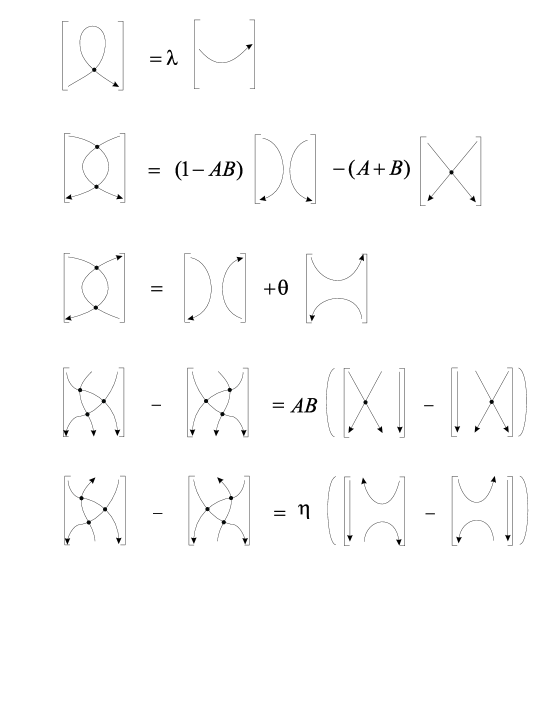
   Fig. 5: Identities for $[]_{R}$.

The following theorem is implicit in [19].

Theorem 3.1

Let $L$ be an oriented link diagram. Then

$$R_{L}(A-B,a)=\sum_{G}A^{i(G)}B^{j(G)}[G]_{R},$$ (5)

where the summation is over all oriented 4-valent plane graphs: $G$’s, obtained from $L$ by applying to each crossing (positive or negative) one of the two replacements as shown in Fig. 6, and $i(G)$ and $j(G)$ are the numbers of positive and negative crossings of $L$ smoothed to form $G$, respectively.

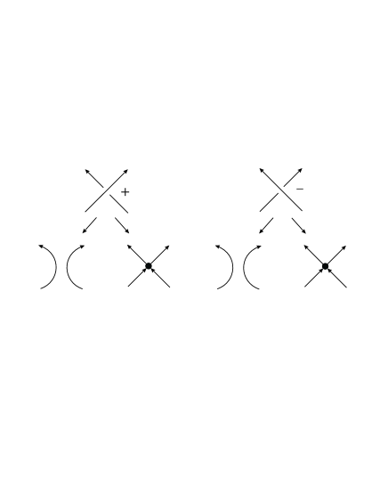
Fig. 6: Two types of replacements of an oriented crossing.

By a little abuse of notations, if we write $[L]=R_{L}$, then we have the following recursive equation as shown in Fig. 7. Note that the subscript $R$ of $[]_{R}$ is omitted.

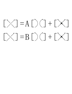
Fig. 7: Recursive equation for $R_{L}$.

3.2 $D$ polynomial

The 3-variable polynomial $[G]_{D}=[G]_{D}(A,B,a)$ for an unoriented 4-valent plane graph $G$ can be defined via the following graphical calculus [19, 5].

Graphical calculus for the $[]_{D}$ polynomial

1. $[\bigcirc]_{D}=1$, where $\bigcirc$ is a free loop.

2. $[G\sqcup\bigcirc]_{D}=\mu[G]_{D}$, where $G\sqcup\bigcirc$ is the disjoint union of an unoriented 4-plane graph $G$ and $\bigcirc$, and $\mu={a-a^{-1}\over A-B}+1$.

3. Let

   $$o = {Aa^{-1}-Ba\over A-B}-(A+B),$$

   $$\gamma = {B^{2}a-A^{2}a^{-1}\over A-B}+AB,$$

   $$\xi = {B^{3}a-A^{3}a^{-1}\over A-B}.$$

   Then identities as shown in Fig. 8 hold:

   

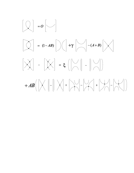
   Fig. 8: Identities for $[]_{D}$.

The following theorem is implicit in [19], and explicit in [5].

Theorem 3.2

Let $L$ be an unoriented link diagram. Then

$$D_{L}(A-B,a)=\sum_{G}A^{i(G)}B^{j(G)}[G]_{D},$$ (6)

where the summation is over all (unoriented) 4-valent plane graphs: $G$’s, obtained from $L$ by applying to each crossing one of the three types of replacements as shown in Fig. 9, and $i(G)$ and $j(G)$ are the numbers of crossings of $L$ of $A$-smoothings and $B$-smoothings used to form $G$, respectively.

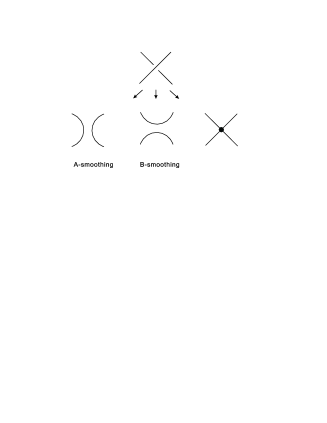
Fig. 9: Three types of replacements of an unoriented crossing.

Similarly, if we write $[L]=D_{L}$, then we have the following recursive equation as shown in Fig. 10.

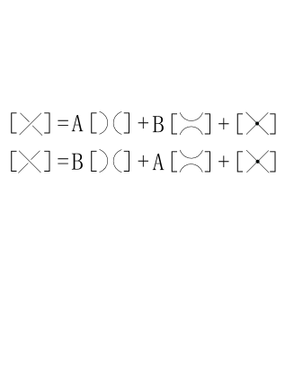
Fig. 10: Recursive equation for $D_{L}$.

4 Jaeger and Wu’s formulae

Let $L$ be an oriented link diagram, the rotation number (also called Whitney degree, see [15], p. 170) rot($L$) of $L$ is equal to the sum of signs for all Seifert circles of $L$ with the convention that the sign is $+1$ if the circle is counterclockwise oriented and the sign is $-1$ if the circle is clockwise oriented. It actually measures the total turn of the unit tangent vector to the underlying plane curves of the link diagram. The rotation number of an oriented 4-valent plane graph is thus equal to that of any oriented link diagram obtained from the graph by converting each vertex into a crossing.

4.1 Jaeger’s formula

Jaeger (see [18], pp. 219-222) established a relation between Kauffman polynomial and Homflypt polynomial, which expresses the $D$ polynomial of a link diagram as the certain weighted sum of Homflypt polynomials of some oriented link diagrams obtained by firstly “splicing” some crossings of the link diagram and then assigning an orientation. Jaeger’s formula can also be found in [7, 25]. Here we give it a slightly different formulation. Note that in this paper we use the normalized versions of the $R$ and $D$ polynomials, while in [18, 7, 25], the authors all dealt with unnormalized versions.

Let $L$ be an unoriented link diagram. We call a segment of the diagram between two adjacent crossings an edge of $L$. An edge orientation of $L$ is balanced if, at each crossing, among four (not necessarily distinct) edges around the crossing, two edges are “in” and two edges are “out”. Up to rotation, there are four possible balanced edge orientations near a crossing: two are crossing-like oriented and the other two are alternatingly oriented. (See Fig. 11.)

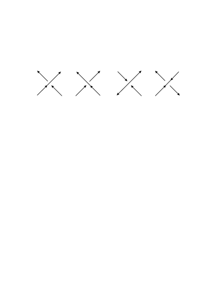
Fig. 11: Balanced edge orientation near a crossing: the first is a positive crossing-like oriented crossing; the second is a negative crossing-like oriented crossing; the third and the fourth are both alternatingly oriented called top outward crossing and top inward crossing, respectively in [25].

Denote by $\mathcal{O}(L)$ the set of all balanced edge orientations of $L$.

Given an $o\in\mathcal{O}(L)$, equipping $L$ with $o$, we obtain $L_{o}$. To obtain oriented link diagrams from $L_{o}$ we need to “splicing” all alternatingly oriented crossings. There are two ways of smoothing a top outward crossing and a top inward crossing of $L_{o}$ as shown in Fig. 12. A resolution $r$ of $L_{o}$ is a choice of $A$ or $B$ smoothing for every top outward and top inward crossing of $L_{o}$. Denote by $\sum(L_{o})$ the set of all resolutions of $L_{o}$. Given a $r\in\sum(L_{o})$, for each top outward and top inward crossing $c$ of $L_{o}$, we define the weight to be

$$[L_{o},r;c]=\left\{\begin{array}[]{ll}q-q^{-1}&\textrm{if $c$ is a top outward crossing and $r$}\\ &\textrm{applies $A$ smoothing to $c$,}\\ q^{-1}-q&\textrm{if $c$ is a top outward crossing and $r$}\\ &\textrm{applies $B$ smoothing to $c$,}\\ 0&\textrm{if $c$ is a top inward crossing.}\end{array}\right.$$

We can take the weight of the unspliced crossing $L_{o}$ to be 1. The total weight $[L_{o},r]$ of the resolution $r$ (applied to $L_{o}$) is defined to be the product of weights of all crossings of $L_{o}$. Denote by $L_{o,r}$ the oriented link diagram obtained by applying $r$ to $L_{o}$.

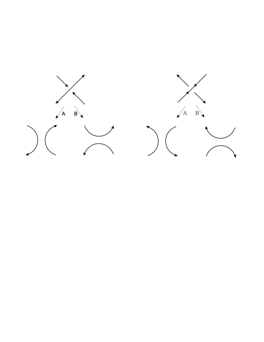
Fig. 12: Two ways of smoothing a top outward crossing and a top inward crossing.

Theorem 4.1

(Jaeger’s Formula) Let $L$ be an unoriented link diagram. Then

$$D_{L}(q-q^{-1},a^{2}q^{-1})=J\sum_{o\in\mathcal{O}(L)}\sum_{r\in\sum(L_{o})}(qa^{-1})^{{\rm rot}(L_{o,r})}[L_{o},r]R_{L_{o,r}}(q-q^{-1},a),$$

where $J={1\over qa^{-1}+q^{-1}a}$.

Remark 4.2

We have two remarks on Theorem 4.1.

1. There is a coefficient $J$ in Theorem 4.1, for we use the normalized Homflypt and Kauffman polynomials in this paper. So

   $$J={\delta\over\mu}={{a-a^{-1}\over q-q^{-1}}\over{a^{2}q^{-1}-a^{-2}q\over q-q^{-1}}+1}={1\over qa^{-1}+q^{-1}a}.$$

2. Since, for $L_{o}$ which contains a top inward crossing and any $r\in\sum(L_{o})$, we have $[L_{o},r]=0$, there are some terms in the right hand of Theorem 4.1 which is equal to 0. In Theorem 4.1, actually we can only consider balanced edge orientations of $L$ which do not contain a top inward crossing. We add some 0 terms in the summation, which, you will see, is important to prove our main Theorem 5.1.

4.2 Wu’s formula

In [25], Wu built a relation between the 3-variable KV polynomial and the 3-variable MOY polynomial of 4-valent rigid vertex spatial graphs. We shall only restrict ourselves to 4-valent plane graphs.

Let $G$ be a 4-valent plane graph. An edge orientation of $G$ is balanced if, at each vertex, among four edges incident with the vertex, two edges are “in” and two edges are “out”. Up to rotation, there are two possible balanced edge orientations near a vertex: one is crossing-like oriented and the other is alternatingly oriented. (See Fig. 13.)

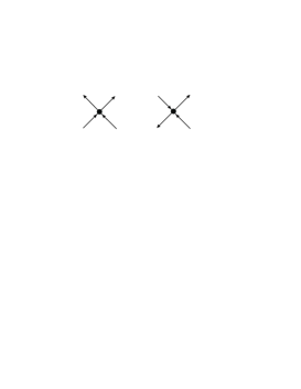
Fig. 13: Balanced edge orientation near a vertex: the first is a crossing-like oriented vertex; the second is an alternatingly oriented vertex.

Denote by $\mathcal{O}(G)$ the set of all balanced edge orientation of $G$.

Given an $o\in\mathcal{O}(G)$, equipping $G$ with $o$, we obtain $G_{o}$. To obtain oriented 4-plane graphs from $G_{o}$ we need to splice all alternatingly oriented vertices. There are two ways of smoothing an alternatingly oriented vertex of $G_{o}$ as shown in Fig. 14. A resolution $r$ of $G_{o}$ is a choice of $L$ or $R$ smoothing of every alternatingly oriented vertex of $G_{o}$. Denote by $\sum(G_{o})$ the set of all resolutions of $G_{o}$. Given a $r\in\sum(G_{o})$, for each alternatingly oriented vertex $v$ of $G_{o}$, we define the weight to be

$$[G_{o},r;v]=\left\{\begin{array}[]{ll}-q&\textrm{if $r$ applies $L$ smoothing to the vertex $v$,}\\ -q^{-1}&\textrm{if $r$ applies $R$ smoothing to the vertex $v$.}\end{array}\right.$$

We can take the weight of crossing-like oriented vertex of $G_{o}$ to be 1. The total weight $[G_{o},r]$ of the resolution $r$ is defined to be the product of weights of all vertices of $G_{o}$. Denote by $G_{o,r}$ the oriented 4-valent plane graph obtained by applying $r$ to $G_{o}$.

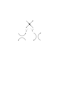
Fig. 14: Two ways of smoothing an alternatingly oriented vertex.

Theorem 4.3

(Wu’s Formula) Let $G$ be an unoriented 4-valent plane graph. Then

$$[G]_{D}(q,q^{-1},a^{2}q^{-1})=J\sum_{o\in\mathcal{O}(G)}\sum_{r\in\sum(G_{o})}(qa^{-1})^{{\rm rot}(G_{o,r})}[G_{o},r][{G_{o,r}}]_{R}(q,q^{-1},a),$$

where $J={1\over qa^{-1}+q^{-1}a}$.

Remark 4.4

Note that $[G_{o},r;v]=-[D_{e},z;v]$ in [25], since by comparing Figs. 7, 10 with Eqs. (1.11) and (1.9) in [25], we know that the $[G]_{R}$ (resp. $[G]_{D}$) is equal to the result of multiplying $(-1)^{|V(G)|}$ and $R(G)$ (resp. $P(G)$) in [25].

5 Two models and their relationship

Now we are in a position to derive two oriented 4-valent graphical models for the Kauffman polynomial. We call the $HJ$ model the summation obtained by applying Jaeger’s formula ($J$) firstly and then Kauffman-Vogel model for the Homflypt polynomial ($H$). Similarly, we call $WF$ model the summation obtained by applying Kauffman-Vogel model for the Kauffman polynomial ($F$) and Wu’s formula ($W$). Let $L$ be an unoriented link diagram.

1. The $HJ$ model: $D_{L}(q-q^{-1},a^{2}q^{-1})$
   

   $$= J\sum_{o\in\mathcal{O}(L)}\sum_{r\in\sum(L_{o})}(qa^{-1})^{{\rm rot}(L_{o,r})}[L_{o},r]\sum_{\ {}_{o,r}\!I}q^{i(_{o,r}I)-j(_{o,r}I)}[_{o,r}I]_{R}(q,q^{-1},a)$$

   $$= J\sum_{o\in\mathcal{O}(L)}\sum_{r\in\sum(L_{o})}\sum_{\ {}_{o,r}\!I}(qa^{-1})^{{\rm rot}(_{o,r}I)}[L_{o},r]q^{i(_{o,r}I)-j(_{o,r}I)}[_{o,r}I]_{R}(q,q^{-1},a),$$

   where the third summation runs over all oriented 4-valent plane graphs: ${}_{o,r}I$’s, obtained from $L_{o,r}$ by applying $H$. The second “$=$” holds since rot($L_{o,r}$)=rot(${}_{o,r}I$) for any ${}_{o,r}I$.

2. The $WF$ model: $D_{L}(q-q^{-1},a^{2}q^{-1})$
   

   $$= \sum_{G}q^{i(G)-j(G)}J\sum_{o\in\mathcal{O}(G)}\sum_{r\in\sum(G_{o})}(qa^{-1})^{{\rm rot}(G_{o,r})}[G_{o},r][{G_{o,r}}]_{R}(q,q^{-1},a)$$

   $$= J\sum_{G}\sum_{o\in\mathcal{O}(G)}\sum_{r\in\sum(G_{o})}q^{i(G)-j(G)}(qa^{-1})^{{\rm rot}(G_{o,r})}[G_{o},r][{G_{o,r}}]_{R}(q,q^{-1},a),$$

   where the first summation runs over all unoriented 4-plane graphs: $G$’s, obtained from $L$ by applying $F$.

Note that in the $HJ$ model, for different orientation $o$, resolution $r$ and different ways of applying $H$ to $L_{o,r}$, the obtained oriented 4-valent plane graphs: ${}_{o,r}I$’s, are all different in the sense that the crossings and edges of $L$ are labeled differently and kept unchanged after splicing some crossings. Let $S$ be the set of all oriented 4-valent plane graphs constructed from $L$ in the $HJ$ model. In other words, the terms in the $HJ$ model are all different. However, in the $WF$ model, there exist many terms whose corresponding $G_{o,r}$’s are the same. In other words, for different $G$, different orientation $o$ and resolution $r$, the obtained $G_{o,r}$’s are not all different.

Furthermore, note that the set of different oriented 4-valent plane in both models are the same: they are both the set of 4-valent plane graphs obtained from $L$ by replacing each an unoriented crossing $c$ of $L$ by one of the following twelve types of configurations: $V_{1}$, $V_{2}$, $V_{3}$, $V_{4}$, $C_{1}$, $C_{2}$, $C_{3}$, $C_{4}$, $A_{1}$, $A_{2}$, $A_{3}$ and $A_{4}$ as shown in Fig. 15. Of course, we demand orientations of all local replacements are compatible on each edge of the underlying 4-valent plane graph of $L$ when we construct oriented 4-valent plane graphs from $L$.

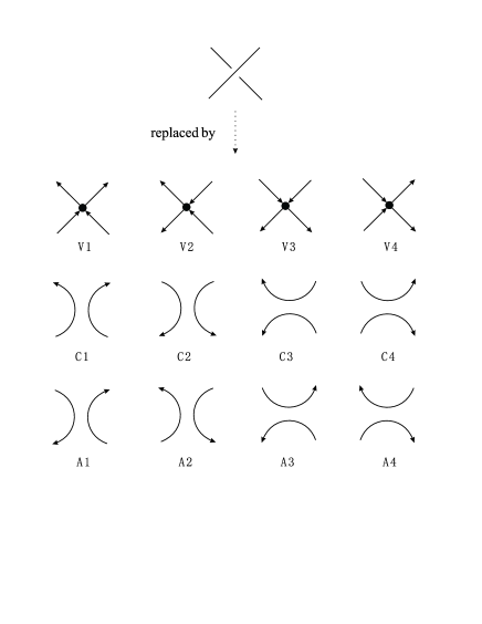
Fig. 15: 12 configurations used to replace an unoriented crossing.

Let $\mathcal{T}=\{G;o,r\}$ be the set of different ways: $G;o,r$’s, of constructing oriented 4-valent plane graphs from $L$, which correspond all terms in the $WF$ model. Now we rewrite the $HJ$ and $WF$ models as the sum

$$\sum_{s\in S}c_{s}[s]_{R}{\ \ \ \textrm{and}\ \ \ }\sum_{G;o,r\in\mathcal{T}}d_{G;o,r}[G_{o,r}]_{R}.$$

Then we have

Theorem 5.1

For each $s\in S$, there exists a subset $T_{s}=\{G;o,r\in\mathcal{T}|s=G_{o,r}\}$ such that $T_{s_{1}}\cap T_{s_{2}}=\emptyset$ for any $s_{1},s_{2}\in s$, $\cup_{s\in S}T_{s}=\mathcal{T}$ and $c_{s}=\sum_{G;o,r\in T_{s}}d_{G;o,r}$.

Proof. We have shown the existence of $T_{s}$ such that $T_{s_{1}}\cap T_{s_{2}}=\emptyset$ for any $s_{1},s_{2}\in s$ and $\cup_{s\in S}T_{s}=\mathcal{T}$ in the preceding several paragraphs. Hence, it suffices for us to prove that $c_{s}=\sum_{G;o,r\in T_{s}}d_{G;o,r}$. Let $s=_{o,r}I$. Recall that

$$c_{s} = J(qa^{-1})^{{\rm rot}(s)}[L_{o},r]q^{i(_{o,r}I)-j({o,r}I)},$$

$$d_{G;o,r} = J(qa^{-1})^{{\rm rot}(G_{o,r})}q^{i(G)-j(G)}[G_{o},r]$$

$$= J(qa^{-1})^{{\rm rot}(s)}q^{i(G)-j(G)}[G_{o},r].$$

Now let

$$c_{HJ} = [L_{o},r]q^{i(_{o,r}I)-j(_{o,r}I)},$$

$$c_{WF} = \sum_{G;o,r\in T_{s}}q^{i(G)-j(G)}[G_{o},r].$$

Then we only need to prove $c_{HJ}=c_{FW}$. We suppose that $s$ is the 4-valent plane graph obtained from $L$ by $v_{i}$ replacements of the configuration $V_{i}$, $c_{i}$ replacements of the configuration $C_{i}$ and $a_{i}$ replacements of the configuration $A_{i}$ for $i=1,2,3,4$.

By applying $J$ firstly then $H$, an unoriented crossing $c$ of $L$ will be replaced by one of eight oriented configurations firstly, then each of the four crossing-like oriented configurations is replaced by one of two configurations (see Fig. 16). The corresponding weight in the product $[L_{o},r]q^{i(_{o,r}I)-j(_{o,r}I)}$ is labeled as the subscript in that figure.

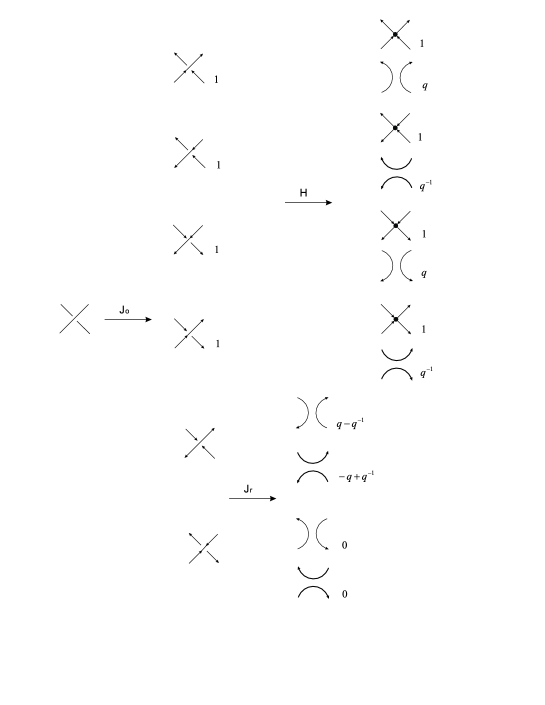
Fig. 16: The $HJ$ model expansion, $J_{o}$ means orientation by applying $J$, $J_{r}$ means resolution by applying $J$.

Similarly, applying $F$ firstly then $W$, an unoriented crossing $c$ of $L$ will be replaced by one of three unoriented configurations: $A$-smoothing, $B$-smoothing and the vertex replacement firstly, then each of the two smoothings is replaced by one of four oriented configurations and the vertex replacement is replaced by one of eight oriented configurations (see Fig. 17). The corresponding weight in $q^{i(G)-j(G)}[G_{o},r]$ is also labeled as the subscript in the figure.

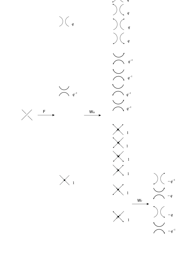
Fig. 17: The $WF$ model expansion, $W_{o}$ means orientation by applying $W$, $W_{r}$ means resolution by applying $W$.

Note that in Figs. 16 and 17, the corresponding weights of $V_{1}$, $V_{2}$, $V_{3}$, $V_{4}$, $C_{1}$, $C_{2}$, $C_{3}$ and $C_{4}$ in the two figures are the same. Now we analyze the remaining four configurations: $A_{1}$, $A_{2}$, $A_{3}$, $A_{4}$. There are two cases:

Case 1. If $a_{2}\neq 0$ or $a_{4}\neq 0$, it is clear that $c_{HJ}=0$. Now we consider $c_{WF}$. Without loss of generality we suppose that $a_{2}\neq 0$. Note that $A_{2}$ appears twice in Fig. 17. This means we can obtain $a_{2}$ $A_{2}$ configurations by selecting $k$ $A_{2}$ configurations via applying $F$ and then selecting the remaining $a_{2}-k$ $A_{2}$ configurations via applying $W$ for any $k=0,1,\cdots,a_{2}$. Note that $\sum_{k=0}^{a_{2}}q^{k}(-q)^{a_{2}-k}=0$. Hence $c_{WF}=0$.

Case 2. Otherwise, it means that $s$ does not contain $A_{2}$ and $A_{4}$ configurations. Similarly, $A_{1}$ and $A_{3}$ appears twice in Fig. 17. Since $(q-q^{-1})^{a_{1}}=\sum_{k=1}^{a_{1}}q^{k}(-q^{-1})^{a_{1}-k}$ and $(-q+q^{-1})^{a_{1}}=\sum_{k=1}^{a_{3}}(-q)^{a_{3}-k}(q^{-1})^{k}$, we have $c_{HJ}=c_{WF}$.

This completes the proof of Theorem 5.1. $\Box$

Theorem 5.1 tells us that many terms of the $WF$ model add up to one term of the $HJ$ model, hence, the $HJ$ model is more efficient than $WF$ model. Now we provide an example to illustrate Theorem 5.1.

Example 5.2

The Hopf link.

We first expand the $R$ polynomial of the Hopf link based on $HJ$ model. There are six different balanced orientations for the Hopf link, and twenty four oriented 4-valent plane graphs (i.e. states) are constructed from the Hopf link (see Fig. 18).

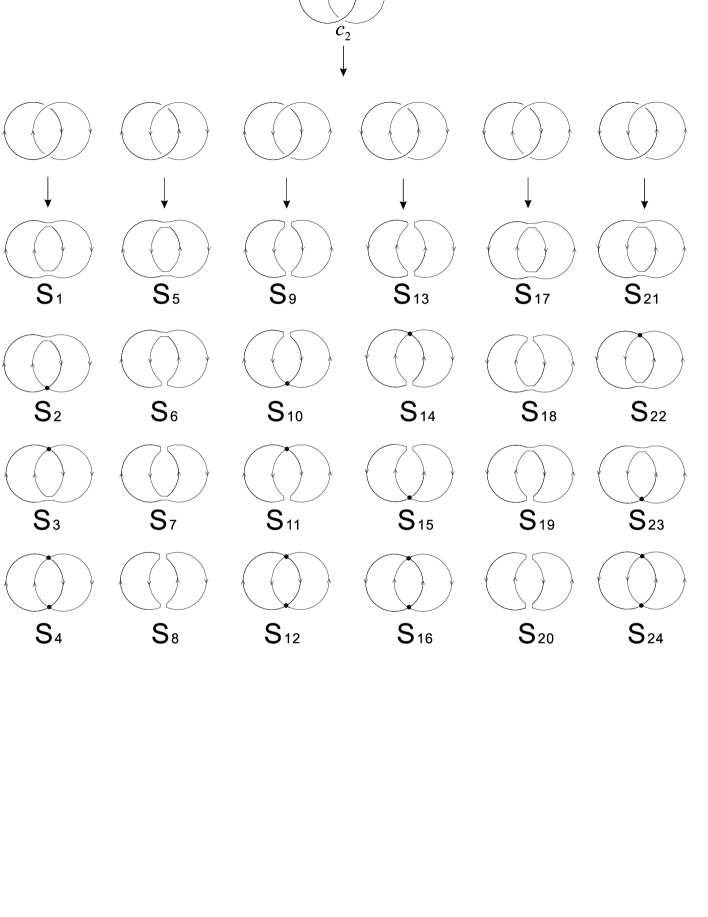
Fig. 18: Hopf link, 6 balanced orientations and 24 states in the $HJ$ model.

We then expand its $R$ polynomial based on $WF$ model. Nine unoriented 4-valent plane graphs by applying $F$ are obtained firstly, then forty eight terms all together are obtained by applying $W$ to each 4-valent plane graph (see Fig. 19).

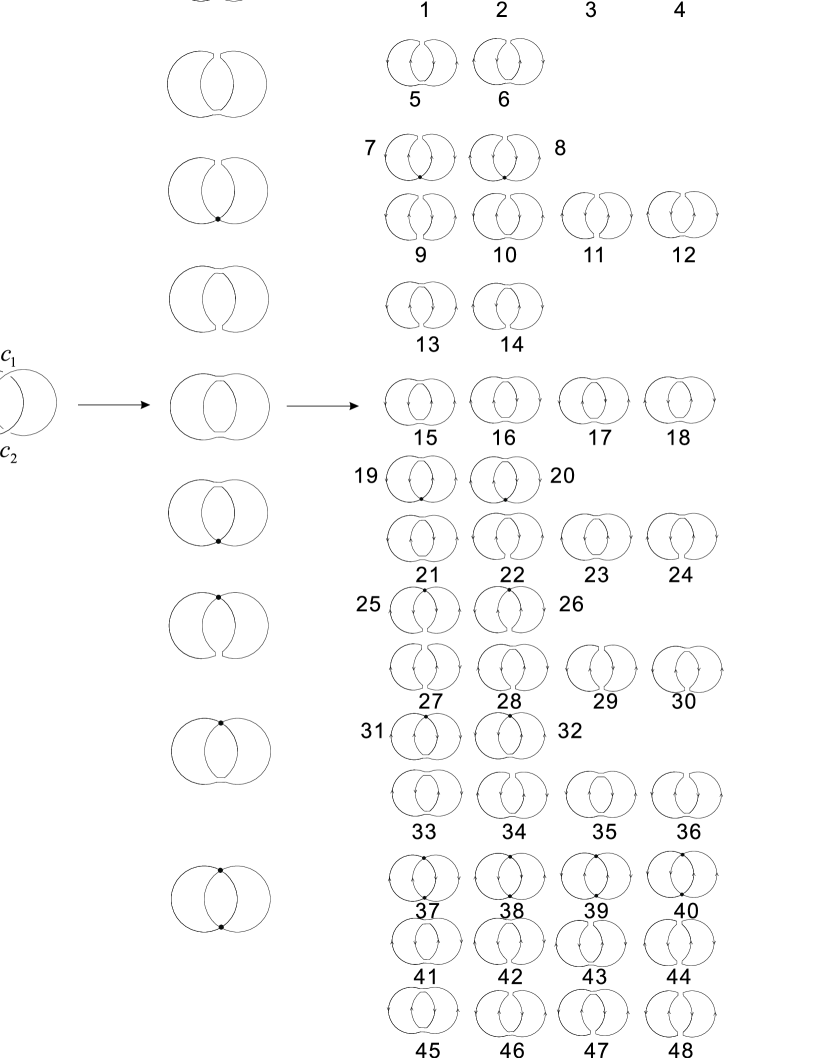
Fig. 19: Hopf link, 9 corresponding unoriented 4-valent plane graphs and 48 terms in the $WF$ model.

For each $s_{i}$, its corresponding weights of the two crossings in $HJ$ model, oriented 4-valent plane graphs corresponding to elements of $T_{s_{i}}$ and the their corresponding weights of two crossings are listed in Table 1. It is easy to verify that $c_{HJ}=c_{WF}$.

$s$ and its weight	Graphs corresponding to elements of $T_{s}$ and their
$[w(c_{1}),w(c_{2})]$	corresponding weights of crossings $c_{1}$ and $c_{2}$
$s_{1}\ [q^{-1},q^{-1}]$	$16\ [q^{-1},q^{-1}]$
$s_{2}\ [q^{-1},1]$	$20\ [q^{-1},1]$
$s_{3}\ [1,q^{-1}]$	$31\ [1,q^{-1}]$
$s_{4}\ [1,1]$	$37\ [1,1]$
$s_{5}\ [q^{-1}-q,q^{-1}-q]$	$18\ [q^{-1},q^{-1}]$, $23\ [q^{-1},-q]$, $33\ [-q,q^{-1}]$, $41\ [-q,-q]$
$s_{6}\ [q^{-1}-q,q-q^{-1}]$	$14\ [q^{-1},q]$, $24\ [q^{-1},-q^{-1}]$, $28\ [-q,q]$, $42\ [-q,-q^{-1}]$
$s_{7}\ [q-q^{-1},q^{-1}-q]$	$06\ [q,q^{-1}]$, $12\ [q,-q]$, $34\ [-q^{-1},q^{-1}]$, $43\ [-q^{-1},-q]$
$s_{8}\ [q-q^{-1},q-q^{-1}]$	$04\ [q,q]$, $11\ [q,-q^{-1}]$, $27\ [-q^{-1},q]$, $44\ [-q^{-1},-q^{-1}]$
$s_{9}\ [q,q]$	$02\ [q,q]$
$s_{10}\ [q,1]$	$08\ [q,1]$
$s_{11}\ [1,q]$	$25\ [1,q]$
$s_{12}\ [1,1]$	$38\ [1,1]$
$s_{13}\ [q,q]$	$01\ [q,q]$
$s_{14}\ [1,q]$	$26\ [1,q]$
$s_{15}\ [q,1]$	$07\ [q,1]$
$s_{16}\ [1,1]$	$39\ [1,1]$
$s_{17}\ [0,0]$	$17\ [q^{-1},q^{-1}]$, $21\ [q^{-1},-q^{-1}]$, $35\ [-q^{-1},q^{-1}]$, $45\ [-q^{-1},-q^{-1}]$
$s_{18}\ [0,0]$	$05\ [q,q^{-1}]$, $10\ [q,-q^{-1}]$, $36\ [-q,q^{-1}]$, $46\ [-q,-q^{-1}]$
$s_{19}\ [0,0]$	$13\ [q^{-1},q]$, $22\ [q^{-1},-q]$, $30\ [-q^{-1},q]$, $47\ [-q^{-1},-q]$
$s_{20}\ [0,0]$	$03\ [q,q]$, $09\ [q,-q]$, $29\ [-q,q]$, $48\ [-q,-q]$
$s_{21}\ [q^{-1},q^{-1}]$	$15\ [q^{-1},q^{-1}]$
$s_{22}\ [1,q^{-1}]$	$32\ [1,q^{-1}]$
$s_{23}\ [q^{-1},1]$	$19\ [q^{-1},1]$
$s_{24}\ [1,1]$	$40\ [1,1]$

Table 1. $s$, $T_{s}$ and corresponding weights.

Now we simplify the $HJ$ model by deleting the 0-terms and obtain

Theorem 5.3

Let $L$ be an unoriented link diagram. Then

$$D_{L}(q-q^{-1},a^{2}q^{-1})=J\sum_{\sigma}\left\{\prod_{c}w(\sigma,c)\right\}(qa^{-1})^{{\rm rot}(\sigma)}[\sigma]_{R}(q,q^{-1},a),$$

where $J={1\over qa^{-1}+q^{-1}a}$, the summation runs over all oriented 4-valent plane graphs obtained from $L$ by replacing each crossing by one of the $V_{1}$, $V_{2}$, $V_{3}$, $V_{4}$, $C_{1}$, $C_{2}$, $C_{3}$, $C_{4}$, $A_{1}$, and $A_{3}$ (see Fig. 15), the product is over all crossings of $L$, and the weight $w(\sigma,c)$ depends on the replacement of $c$ in $\sigma$ and is shown as the subscript in Fig. 16.

6 Trivalent graphical models

There are also trivalent graphical models for both the $R$ and $D$ polynomial, see [21, 8] and [4] respectively. By unoriented trivalent graph, we mean a trivalent undirected graph having two types of edges, “thick” edges and “common” edges such that there is exactly one “thick” edge incident to each vertex. We take free loops to be special cases of unoriented trivalent graphs. Clearly there is a many-to-one correspondence $f$ between such unoriented trivalent graphs and unoriented 4-valent graphs and $f$ maps the unoriented trivalent graph to the unoriented 4-valent graph obtained from the unoriented trivalent graph by contracting all thick edges. Under this correspondence and restrict to planar graphs, by comparing the graphical calculus in this paper with Eqs. (2.1)-(2.5) in [4], you will see that the 3-variable polynomial $P(G)$ in [4] and the 3-variable graph polynomial $[f(G)]_{D}$ in [19] are completely the same. Clearly, for the $D$ polynomial there is a bijection between terms of trivalent graphical model [4] and terms of 4-valent graphical model [19]. Hence the trivalent graphical model and the 4-valent graphical model of the $D$ polynomial are essentially the same.

As for the $R$ polynomial, the relation between the trivalent graphical model and the 4-valent graphical model is not very immediate. As far as I know there is no trivalent graphical model for the whole Homflypt polynomial, we only consider the special case of the so-called Homflypt $n$-specializations, that is, we put $z=q-q^{-1}$ and $a=q^{n}$ in the $R$ polynomial. In [21], Murakami, Ohtsuki and Yamada defined an invariant (we call it MOY polynomial) of colored, oriented, trivalent plane graphs. In [8], Freitas only considered a special case which only uses colors 1 and 2 and called them classic graphs. Note that edges colored 1 correspond to “common” edges and edges colored 2 correspond to “thick” edges. In this special case, the corresponding MOY polynomial is called the $\Gamma$-bracket.

Theorem 6.1

Let $L$ be an oriented link diagram. Then

$$R_{L}(q-q^{-1},q^{n})=q^{w(L)}{1\over[n]}\sum_{G}(-q^{-1})^{s(G)}(-q)^{t(G)}<G>_{n},$$ (7)

where $w(L)$ is the writhe of $L$, $[n]=q^{-(n-1)}+q^{-(n-3)}+\cdots+q^{n-3}+q^{n-1}={q^{n}-q^{-n}\over q-q^{-1}}$, the summation is over all $G$’s obtained from $L$ by replacing each crossing by one of the two configurations shown as in Fig. 20, $s(G)$ (resp. $t(G)$) is the number of positive (resp. negative) non-smoothed crossings of $L$ to form $G$, $<G>_{n}$ is the $\Gamma$-bracket of the classic graph $G$.

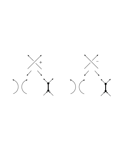
Fig. 20: Two types of replacements to construct the classic graphs.

Proof. Theorem 6.1 is implicit in [8]. It can be obtained by combining Eqs. (2.12), (2.16) and (2.17) with the fact that the $R$ polynomial in this paper is the normalized regular invariant of the Homflypt polynomial. $\Box$

Now we simplify Eq. (7) as follows.

$$R_{L}(q-q^{-1},q^{n}) = q^{w(L)}\sum_{G}(-q^{-1})^{s(G)}(-q)^{t(G)}{1\over[n]}<G>_{n}$$ (8)

$$= q^{w(L)}\sum_{G}q^{t(G)-s(G)}{(-1)^{|V(G)|}\over[n]}<G>_{n}$$

$$= \sum_{G}q^{i(G)-j(G)}{(-1)^{|V(G)|}\over[n]}<G>_{n},$$

where $V(G)$ is the vertex set of $G$ and $i(G)$ (resp. $j(G)$) is the number of positive (resp. negative) crossings smoothed to obtain $G$.

Note that by contracting all “thick” edges of a classic graph, we obtain an oriented 4-valent plane graph. By putting $A=q$, $B=q^{-1}$, $a=q^{n}$ in Theorem 3.1, it is very similar to Eq. (8). By comparing Eqs. (3.1)-(3.5) in [8] and graphical calculus for $[]_{R}$, it is not difficult for us to verify that ${(-1)^{|V(G)|}\over[n]}<G>_{n}=[f(G)]_{R}(q,q^{-1},q^{n})$ . We leave the details to the readers. Note that for the Homflypt $n$-specializations, the identity $(iii)^{\prime}$ in Fig. 5 is redundant.

Therefore, for the Homflypt $n$-specializations, the trivalent graphical model in [8] and the the 4-valent trivalent graphical model are consistent. Clearly, for the $R$ polynomial there is also a bijection between terms of trivalent graphical model [21, 8] and terms of 4-valent graphical model [19].

Acknowledgements

This paper was completed during my visiting the Lafayette College. I would like to thank Professor L. Traldi for introducing me to the study of relations among various models of link polynomials and some helpful conversations and comments. This work was also partially supported by Grants from the National Natural Science Foundation of China (No. 10831001) and the Fundamental Research Funds for the Central Universities (No. 2010121007).

References

- [1] J. W. Alexander, Topological invariants of knots and links, Trans. Amer. Math. Soc. 30 (1928) 275-306.
- [2] J. A. Bondy and U. S. R. Murty, Graph theory with applications, The Macmillan press ltd, 1976.
- [3] R. D. Brandt, W. B. R. Lickorish and K. C. Millett, A polynomial invariant for unoirened knots and links, Invent. Math. 74 (1986) 563-573.
- [4] C. Caprau, J. Tipton, The Kauffman polynomial and trivalent graphs, arXiv:1107.1210v2 [math.GT] 11 Jul 2011.
- [5] R. P. Carpentier, From planar graphs to embedded graphs-a new approach to Kauffman and Vogel’s polynomial, J. Knot Theory Ramifications 9(8) (2000) 975-986.
- [6] J. H. Conway, An enumeration of knots and links, and some of their algebraic properties, Computational Problems in Abstract Algebra, Pergamon Press, New York (1970) 329-358.
- [7] E. Ferrand, On Legendrian knots and polynomial invariants, Proc. Amer. Amer. Soc. 130(4) (2001) 1169-1176.
- [8] N. R. B. Freitas, A combinatorial approach to the Homfly -specializations, 2008.
- [9] P. Freyd, D. Yetter, J. Hoste, W. B. R. Lickorish, K. Millett, and A. Ocneanu, A new polynomial invariant of knots and links, Bull. Amer. Math. Soc. (N.S.) 12(2) (1985) 239-246.
- [10] C. F. Ho, A new polynomial invariant for knots and links-preliminary report, Abstracts Amer. Math. Soc. 6 (1985) 300.
- [11] S. Huggett, On tangles and matroids, J. Knot Theory Ramifications 14(7) (2005) 919-929.
- [12] F. Jaeger, Tutte polynomials and link polynomials, Proc. Amer. Math. Soc. 103 (1988) 647-654.
- [13] V. F. R. Jones, A polynomial invariant for knots via Von Neumann algebras, Bull. Amer. Math. Soc. 12 (1985) 103-111.
- [14] L. H. Kauffman, State models and the Jones polynomial, Topology 26 (1987) 395-407.
- [15] L. H. Kauffman, On knots, Annals of Mathematics Studies, No. 115, Princeton University Press, Princeton, New Jersey, 1987.
- [16] L. H. Kauffman, Invariants of graphs in three-space, Trans. Amer. Math. Soc. 311(2) (1989) 697-710.
- [17] L. H. Kauffman, An invariant of regular isotopy, Trans. Amer. Math. Soc. 318(2) (1990) 417-471.
- [18] L. H. Kauffman, Knots and Physics, World Scientifc, 1991.
- [19] L. H. Kauffman, P. Vogel, Link polynomials and a graphical calculus, J. Knot Theory Ramifications 1(1) (1992) 59-104.
- [20] W. B. R. Lickorish, Some link-polynomial relations, Math. Proc. Phil. Soc. 105 (1989) 103-107.
- [21] H. Murakami, T. Ohtsuki, S. Yamada, Homfly polynomial via an invariant of clored plane graphs, Enseign. Math. 44 (1998) 325-360.
- [22] J. H. Przytycki, P. Traczyk, Invariants of links of Conway type, Kobe J. Math. 4 (1987) 115-139.
- [23] M. B. Thistlethwaite, A spanning tree expansion of the Jones polynomial, Topology 26 (1987) 297-309.
- [24] W. T. Tutte, A contribution to the theory of chromatic polynomials, Canad. J. Math. 6 (1954) 80-91.
- [25] H. Wu, On the Kauffman-Vogel and the Murakami-Ohtsuki-Yamada graph polynomials, arXiv:1107.5333v1 [math.GT] 26 July 2011.