Recurrence of particles in static and time varying oval billiards

Abstract

Dynamical properties are studied for escaping particles, injected through a hole in an oval billiard. The dynamics is considered for both static and periodically moving boundaries. For the static boundary, two different decays for the recurrence time distribution were observed after exponential decay for short times: A changeover to: (i) power law or; (ii) stretched exponential. Both slower decays are due to sticky orbits trapped near KAM islands, with the stretched exponential apparently associated with a single group of large islands. For time dependent case, survival probability leads to the conclusion that sticky orbits are less evident compared with the static case.

1 Introduction

Billiards are dynamical systems where an ensemble of moving particles do not interact with each other and suffer specular reflections with the boundary [1, 2]. Applications of billiards can be made to different physical systems including experiments in reflection of light from mirrors [3], superconducting [4] and confinement of electrons in semiconductors by electric potentials [5, 6], wave guides [7], microwave billiards [8, 9], ultra-cold atoms trapped in a laser potential [10, 11, 12, 13] and also mesoscopic quantum dots [14].

Billiard dynamics falls into three main classes namely: (i) regular [2]; (ii) intermittent [15] or; (iii) totally chaotic behavior [16]. Two examples of case (i) are the circular billiard [1], which preserves both the energy and angular momentum, and the elliptic billiard which preserves the energy and the product of the angular momenta about the two foci [2]. Case (ii) holds for typical billiard shapes, including many models considered so far [17, 18, 19, 20], producing a mixed phase space structure in the sense that elliptic islands with fractal boundaries, generally surrounded by a chaotic sea that often is confined by invariant spanning curves, can all be observed. The latter case (iii) includes Sinai [21] dispersing billiards with corners as the diamond [22], or periodically extended such as the finite horizon Lorentz gas [23, 24]. Billiards may also be constructed that are fully chaotic according to the defocusing mechanism [16, 25]. However many famous examples such as the Sinai billiard consisting of a square with a circular obstacle (or the equivalent infinite horizon Lorentz gas [26, 27] and the Bunimovich stadium have a regular family of periodic orbits, thus making the dynamics intermittent as in case (ii), even though the phase space is a single chaotic ergodic component. This makes them analytically tractable models for mixed systems, similar to the more recently introduced mushroom billiards, which have chaotic and regular regions of phase space, but separated by smooth (rather than fractal) boundaries [28, 29].

A time perturbation to the boundary may be considered, for example due to thermal vibrations in solids [30], with amplitude and typical frequency related to the temperature. Depending on the type and shape of the billiard, such a time-dependence leads to the so called Fermi acceleration (FA) [31]. This phenomenon consists in the unlimited energy growth of the bouncing particle upon collisions with the, presumably, infinitely heavy moving boundary. Several different kinds of perturbation can be considered in different billiard-like models [32, 33, 34, 35, 36]. As claimed in the Loskutov-Ryabov-Akinshin (LRA) conjecture [37], if the dynamics of the particle is chaotic while the boundary is static, thus this is a sufficient condition to observe FA when a time perturbation to the boundary is introduced. Recently it was shown [38] that even a time-dependent elliptic billiard, which is integrable for the static boundary, can also generate FA thanks to the appearance of a stochastic layer replacing the separatrix curve in the phase space. Moreover, the existence a heteroclinic orbit could extend the LRA conjecture [39] and the unlimited energy growth can be observed even in (some) integrable billiards. The occurrence of an exponential FA was reported in a time varying rectangular billiard [40], which was latter explained [41] as due to a sequence of highly correlated motion which consists of alternating phases with free propagation motion along the invariant spanning curves of the Fermi-Ulam model; see Ref. [42] for the localization of such curves for a family of mappings whose angle is a diverging function of the action in the limit of vanishing action, including the Fermi-Ulam model.

When a hole is introduced in the boundary therefore letting the particle leave the billiard region, we may consider related problems of escape (initial conditions in the billiard) or recurrence (initial conditions at the hole); here we consider recurrence, but virtually all of the following discussion applies also to escape, with a different exponent in the distributions if there is a power law decay. It is known that, for fully chaotic dynamics, the recurrence time distribution, i.e. the time the particle stays confined in the billiard domain, is characterized by an exponential decay [43]. On the other hand, for intermittent including mixed phase space dynamics where there is stickiness, generated from a finite time (but arbitrarily long) trapping near periodic/elliptic regions, a power law decay is observed [44]. Recently, an investigation of a mushroom billiard led to the characterization of families of marginally unstable periodic orbits [29] responsible for trapping the particle in sticky domains, including their effects on the escape problem. Moreover, for a time dependent potential well [45], the dynamics of the particle is shown to be fully chaotic for the low energy domain and reaching elliptic islands as far as the energy increases until finding a limitation marked by the existence of an invariant spanning curve. For the time dependent potential well, a hole in the energy space was introduced letting the particle escape. Therefore for the low energy regime an exponential decay was observed while a slower decay characterized either as a power law or stretched exponential marks the regime of higher energy and consequently long time. Thus opening a billiard by considering particles escaping through a hole is a good means of identifying and describing various kinds of intermittency present in the dynamics.

The oval considered here is defined by a finite Fourier series in polar coordinates, and the mixed phase space of oval billiards was first described by Berry in 1981 [15]. Since then it has remained a popular example of a billiard with mixed phase space, including for generalizations to time dependent boundaries [46] and wave chaos in theory [47] and microresonator experiments [48]. In this paper we revisit the oval billiard considering both the static and time-dependent boundary. We consider a hole for the first time, seeking to understand and describe some properties of particles returning to the hole.

This paper is organized as follows. In Sec. 2, we describe the model with fixed boundary, detailing results for the recurrence times. Section 3 considers the moving boundary where the equations of the mapping are derived. The results for the recurrence times are discussed here also. Final remarks and conclusions are presented in Sec. 4.

2 The static oval billiard, the mapping and escaping particles

The model we consider in this section consists of a classical particle confined to move in a domain which the radius of the boundary is given by the following equation in polar coordinates

$$R(\theta,\epsilon,p)=1+\epsilon\cos(p\theta)~{},$$ (1)

where $\epsilon$ is the amplitude of the circle’s perturbation, $\theta$ is the angular coordinate and $p>0$ is an integer. For the parameter $\epsilon=0$ the circular billiard is obtained leading to a foliated phase space [1]. Therefore chaos is not observed. In the case of $\epsilon\neq 0$ but considering $\epsilon<\epsilon_{c}=1/(p^{2}+1)$, the billiard is convex, and the phase space contains both elliptic islands, invariant spanning curves corresponding to rotating orbits (also called whispering gallery orbits) and chaotic regions [49] while for $\epsilon\geq\epsilon_{c}$ the billiard is no longer convex; all the invariant tori are destroyed [19] however some elliptic islands survive.

The dynamics of the particle is described by a two-dimensional nonlinear area preserving map $T$ for the variables $(\theta_{n},\alpha_{n})$ where $\theta_{n}$ is the angular position of the particle and $\alpha_{n}$ is the angle that the trajectory of the particle does with respect to the tangent vector of the boundary at the angular position $\theta_{n}$ (see Fig. 1). The index $n$ corresponds to the $n^{th}$ collision of the particle with the boundary. Using polar coordinates one has that $X(\theta_{n})=\left[1+\epsilon\cos(p\theta_{n})\right]\cos(\theta_{n})$ and $Y(\theta_{n})=\left[1+\epsilon\cos(p\theta_{n})\right]\sin(\theta_{n}).$ For an initial condition $(\theta_{n},\alpha_{n})$, the angle between the tangent and the boundary at the position $X(\theta_{n})$ and $Y(\theta_{n})$ with respect to the horizontal is $\phi_{n}=\arctan\left[Y^{\prime}(\theta_{n})/X^{\prime}(\theta_{n})\right]$. Between collisions, the particle travels with a constant velocity along a straight line until reaches the boundary. The equation that gives the trajectory of the particle is

$$Y(\theta_{n+1})-Y(\theta_{n})=\tan(\alpha_{n}+\phi_{n})[X(\theta_{n+1})-X(\theta_{n})],$$ (2)

where $\phi_{n}$ is the slope of the tangent vector measured with respect to the positive X-axis, $X(\theta_{n+1})$ and $Y(\theta_{n+1})$ are the new rectangular coordinates of the collision point at $\theta_{n+1}$, which is numerically obtained as solution of Eq. (2). The angle between the trajectory of the particle and the tangent vector to the boundary at $\theta_{n+1}$ is

$$\alpha_{n+1}=\phi_{n+1}-(\alpha_{n}+\phi_{n}).$$ (3)

Figure 1: Illustration of the angles that describe the dynamics and an escaping trajectory.

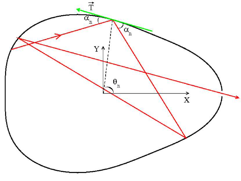
Figure 1 illustrates the corresponding angles and a escaping particle from the billiard. The mapping that describes the dynamics of the model is thus given by

$$T:\left\{\begin{array}[]{ll}F(\theta_{n+1})=R(\theta_{n+1})\sin(\theta_{n+1})-Y(\theta_{n})-\\ ~{}~{}~{}~{}~{}~{}\tan(\alpha_{n}+\phi_{n})[R(\theta_{n+1})\cos(\theta_{n+1})-X(\theta_{n})],{}{}\\ \alpha_{n+1}=\phi_{n+1}-(\alpha_{n}+\phi_{n})\end{array}\right.$$ (4)

where $\theta_{n+1}$ is numerically obtained as solution of $F(\theta_{n+1})=0$ with $R(\theta_{n+1})=1+\epsilon\cos(p\theta_{n+1})$ and $\phi_{n+1}=\arctan[Y^{\prime}(\theta_{n+1})/X^{\prime}(\theta_{n+1})]$.

A typical phase space for the static version for different control parameters together with a visualization of a period three orbit is shown in Fig. 2.

Figure 2: Phase space for the oval billiard for the control parameters: (a) $\epsilon=0.07$ and (b) $\epsilon=0.1$. (c) shows a typical periodic orbit and (d) a zoom-in of a specific region of (b).

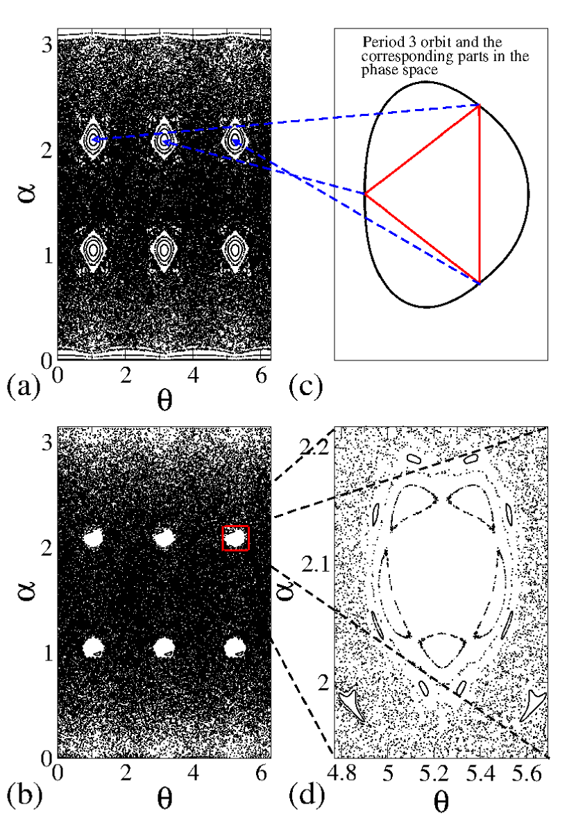
The parameters used in the figure were $p=3$ and: (a) $\epsilon=0.07<\epsilon_{c}$, (b) $\epsilon=0.1=\epsilon_{c}$. Figure 2(c) shows a period three orbit indicating corresponding region in the phase space of (a) while (d) shows zoom-in of a region near a elliptic island of (b).

Let us now consider that the boundary has a hole through which the particles are injected and can escape, as shown in Fig. 1. We assume the hole is localized in $\theta\in(0,h)$ where $h$ is a parameter. We simulated different values of $h\leq\pi/10$ however in this paper we fix it at $h=0.1$. The procedure used to consider the escape of the particles assumes the evolution of an ensemble of initial conditions. Indeed we consider $10^{6}$ different initial conditions in a window where $10^{3}$ $\theta_{0}$ are uniformly distributed along $\theta_{0}\in(0,h)$ while a window of $10^{3}$ different $\alpha_{0}$ also uniformly distributed along $\alpha_{0}\in(0,\pi)$. Each one of them was let to evolve a maximum of $10^{6}$ collisions with the boundary, if it did not escape before. When the particle reaches the region of the hole for the first time, the number of collisions with the boundary spent up to that point is registered and the particle is assumed to escape. A new initial condition is then started and the procedure is repeated until all the ensemble is exhausted. The histogram of frequency of escaping particles, represented as $H(n)$ is shown in Fig. 3(a) for three different parameters, as labeled in the figure.

Figure 3: (a) Histogram of frequency for the escaping orbits from the billiard. (b) Corresponding survival probability, obtained by integration of the histogram shown in (a). The parameters used were $p=3$ and $\epsilon=0.07<\epsilon_{c}$, $\epsilon=0.1=\epsilon_{c}$ and $\epsilon=0.13>\epsilon_{c}$.

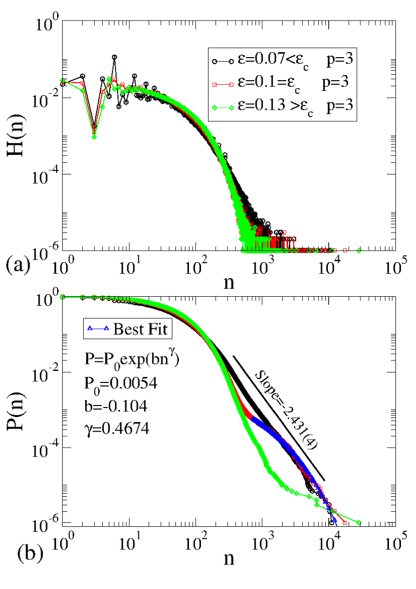
For a fixed $p=3$, the parameter $\epsilon=0.07<\epsilon_{c}$ causes the phase space to have both elliptic islands as well as invariant spanning curves [19] corresponding to the so called whispering gallery orbits. The presence of the elliptic islands leads the dynamics of some initial conditions to experience a sticky behavior that can be long. The invariant spanning curves are destroyed for the cases of $\epsilon=0.1$ and $\epsilon=0.13$. Figure 3(a) shows the behavior of the histogram of escaping orbits. The horizontal axis denotes the number of collisions the particle suffered with the boundary before escaping while the vertical one corresponds to the fraction of orbits which escaped at the $n^{\rm th}$ collision. Given that $p=3$ one can see that the histogram shows a lower value for three bounces with boundary as compared with $n=2$ and $n=4$. This reduction is related to the stability of period three orbits in the phase space, therefore trapping the particle close to this region. For large $n$ we see a long tail which corresponds to sticky orbits. The integration of such histogram gives the so called cumulative recurrence time distribution, which is defined as

$$P={1\over N}{\sum_{j=1}^{N}{N_{\rm rec}(n)}}~{},$$ (5)

where the summation is taken along the ensemble of $N=10^{6}$ different initial conditions. $N_{\rm rec}(n)$ denotes the number of initial conditions that do not escape through the hole (ie recur) until a collision $n$. When Eq. (5) is evaluated in a fully chaotic dynamics its behavior is an exponential [43] while for a mixed phase space where intermittent orbits exist along the phase space a power law is observed [44]. We have shown recently [50] that the existence of elliptic islands may also lead to a stretched exponential decay. Figure 3(b) shows the behavior of three curves of $P(n)~{}vs~{}n$ for the same set of control parameters used in Fig. 3(a). For $\epsilon=0.07<\epsilon_{c}$ the decay is exponentially fast at the beginning until about $200$ collisions of the particle with the boundary when the curve changes to a slower decaying regime marked by a power lay with exponent $-2.431(4)$. For $\epsilon=0.1=\epsilon_{c}$, the invariant spanning curves creating the whispering gallery orbits are destroyed. The decay of $P$ at the beginning is the same for $\epsilon=0.07$ when a hump appeared around $n\cong 500$ lasting until $n\cong 1500$. Indeed the hump is described by a stretched exponential of the type

$$P=P_{0}\exp(b~{}n^{\gamma})$$ (6)

with the coefficients $P_{0}=0.0054$, $b=-0.104$ and $\gamma=0.4674\cong 0.5$. From the $10^{6}$ different initial conditions, the region corresponding to the hump is due to $947$ initial conditions. The major part of the trapping happens near a period three orbit as shown in Fig. 4(a) with the corresponding sticky orbit plotted in Fig. 4(b).

Figure 4: Plot of a typical long-lived orbit in the billiard (a,c) and its corresponding representation in the phase space (b,d) for the parameters $p=3$ $h=0.1$ and: (a,b) $\epsilon=0.1=\epsilon_{c}$; (c,d) $\epsilon=0.13>\epsilon_{c}$.

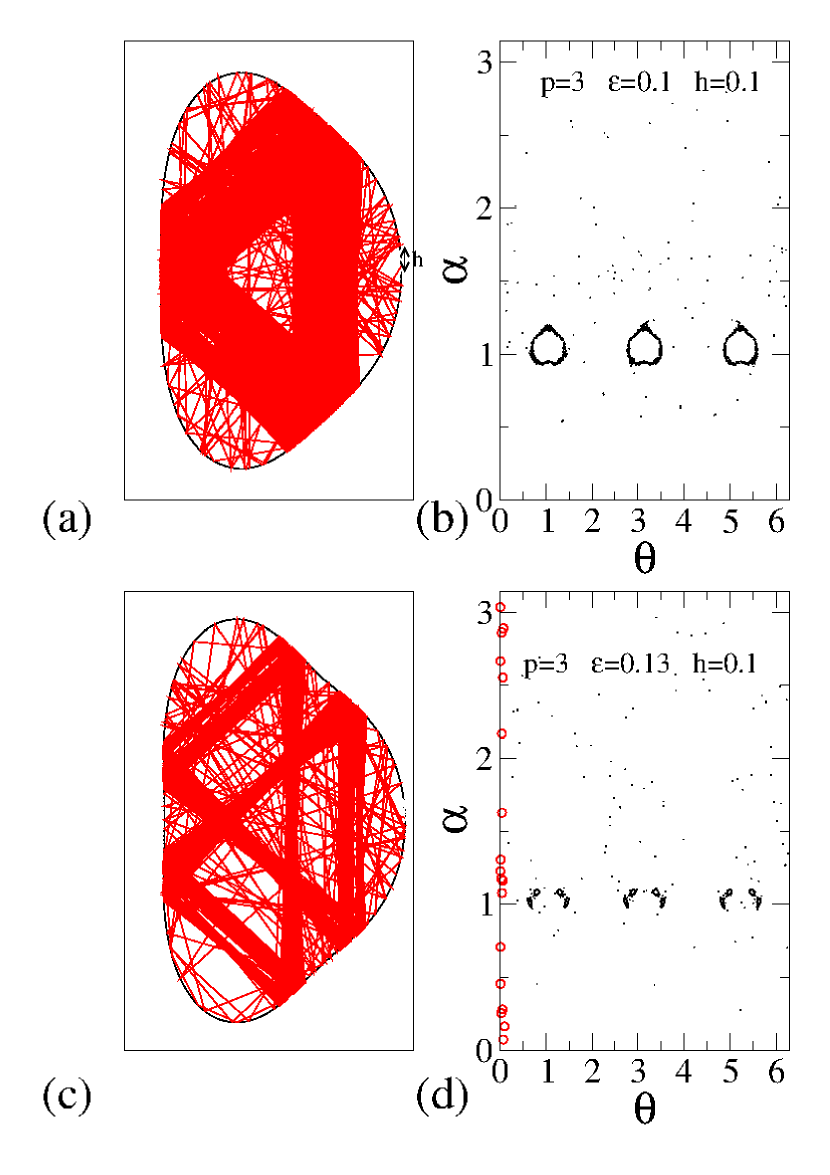
Finally, for $\epsilon=0.13>\epsilon_{c}$ the elliptic regions in the phase space are reduced and the recurrence distribution decays rapidly at first. After $n>1360$, some of the initial conditions are trapped for long time in a sticky region. The few orbits trapped for a long time were mostly observed near a period twelve orbit, as shown in Fig. 4(c) with its corresponding plot in the phase space shown in Fig. 4(d).

3 Time dependent oval billiard and escaping particles results

This section is devoted to discussing the recurrence time distribution of the time-dependent oval billiard. We first construct the mapping that gives the precise description of the dynamics. The radius of the boundary in polar coordinates, to include the time-dependence, is now written as

$$R_{b}(\theta,t)=1+\epsilon[1+a\cos(t)]\cos(p\theta)~{},$$ (7)

where $a$ corresponds to the amplitude of oscillation of the boundary. The introduction of the time perturbation to the boundary produces two new additional variables that have to be considered, namely: (i) the velocity of the particle, $V$, and the time $t$. The map describing the dynamics has now four dynamical variables, i.e. $T(\theta_{n},\alpha_{n},V_{n},t_{n})=(\theta_{n+1},\alpha_{n+1},V_{n+1},t_{n+1})$. Supposing the initial conditions $(\theta_{n},\alpha_{n},V_{n},t_{n})$ are given, a similar procedure as made in the previous section can be used to describe the position and trajectory of the particle. Then the instant of the collision is obtained by the numerical solution of the following equation

$$R_{p}(\theta,t)=R_{b}(\theta,t)~{},$$ (8)

where $R_{b}(\theta,t)=1+\epsilon[1+a\cos(t_{n}+t)]\cos(p\theta_{p})$ and $R_{p}(t)=\sqrt{X^{2}_{p}(t)+Y^{2}_{p}(t)}$ with the corresponding angle $\theta_{p}=\arctan[Y_{p}(t)/X_{p}(t)]$, $X_{p}(t)=X(\theta_{n},t_{n})+|\vec{V}_{n}|\cos(\phi_{n}+\alpha_{n})(t-t_{n})~{},$ and $Y_{p}(t)=Y(\theta_{n},t_{n})+|\vec{V}_{n}|\sin(\phi_{n}+\alpha_{n})(t-t_{n})~{},$ with $t\geq t_{n}$.

The angular coordinate at the new collision, $\theta_{n+1}$, is numerically obtained from Eq. (8) via a numerical procedure similar to the molecular dynamics method leading to an accuracy of $10^{-12}$ in the time of the collision. Given $\theta_{n+1}$, the time at the collision is written as

$$t_{n+1}=t_{n}+{{[(\Delta X)^{2}+(\Delta Y)^{2}]^{1/2}}\over{v_{n}}}~{}.$$ (9)

where $\Delta X=X_{p}(\theta_{n+1})-X_{p}(\theta_{n})$ and $\Delta Y=Y_{p}(\theta_{n+1})-Y_{p}(\theta_{n})$. The velocity of the moving boundary is given by

$$\vec{v}_{b}(t_{n+1}) = -\epsilon a\sin(t_{n+1})\cos(p\theta_{n+1})$$ (10)

$$\times [\cos(\theta_{n+1})\vec{i}+\sin(\theta_{n+1})\vec{j}]~{}.$$

Figure 5: Plot of five snapshots of a trajectory for an escaping particle in the time varying billiard. The control parameters used, for visual purposes, were $p=3$, $\epsilon=0.1$ and $a=0.8$.

Figure 6: (a) Histogram of frequency for the escaping orbits from the billiard. (b) Corresponding survival probability, obtained by integration of the histogram shown in (a). The parameters used were $p=3$ and $\epsilon=0.07<\epsilon_{c}$, $\epsilon=0.1=\epsilon_{c}$ and $\epsilon=0.13>\epsilon_{c}$ and $a=0.1$.

The reflection laws used are

$$\vec{V}^{\prime}_{n+1}\cdot\vec{T}_{n+1}=\vec{V}^{\prime}_{n}\cdot\vec{T}_{n+1}~{},$$ (11)

$$\vec{V}^{\prime}_{n+1}\cdot\vec{N}_{n+1}=-\vec{V}^{\prime}_{n}\cdot\vec{N}_{n+1}~{},$$ (12)

where the upper prime denotes the variables are represented in the moving referential frame. From Eq. (11) one concludes that the tangent component of the velocity does not indeed suffers any modification after the impact. Returning to the inertial frame of reference, we obtain that

$$\vec{v}_{n+1} \cdot \vec{T}_{n+1}=v_{n}[\cos(\alpha_{n}+\phi_{n})\cos(\phi_{n+1})]+$$ (13)

$$+ v_{n}[\sin(\alpha_{n}+\phi_{n})\sin(\phi_{n+1})]~{}.$$

Considering Eq. (12), in the rest referential frame, the normal component of the velocity of the particle is

$$\vec{v}_{n+1} \cdot \vec{N}_{n+1}=-v_{n}[-\cos(\alpha_{n}+\phi_{n})\sin(\phi_{n+1})]+$$

$$+ v_{n}[\sin(\alpha_{n}+\phi_{n})\cos(\phi_{n+1})]-$$

$$- 2\epsilon a\sin(t_{n+1})\cos(p\theta_{n+1})[-\cos(\theta_{n+1})\sin(\phi_{n+1})]-$$

$$- 2\epsilon a\sin(t_{n+1})\sin(\theta_{n+1})\cos(\phi_{n+1})]~{}.$$

The velocity of the particle immediately after the impact is

$$v_{n+1}=\sqrt{(\vec{v}_{n+1}\cdot\vec{T}_{n+1})^{2}+(\vec{v}_{n+1}\cdot\vec{N}_{n+1})^{2}}~{},$$ (14)

and finally, the angle that the particle leaves the boundary, measured with respect to a tangent to the point $\theta_{n+1}$ is written as

$$\alpha_{n+1}=\arctan\left[{{\vec{v}_{n+1}\cdot\vec{N}_{n+1}}\over{\vec{v}_{n+1}\cdot\vec{T}_{n+1}}}\right]~{}.$$ (15)

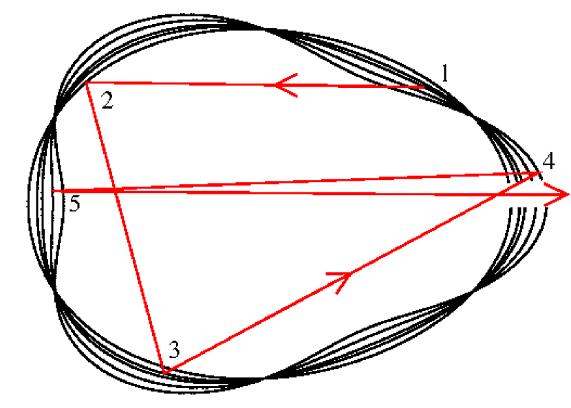
For $a\neq 0$ the particle can gain or lose energy upon collisions with the boundary and given that the phase space has chaotic components, unlimited energy growth is observed [51] therefore confirming the LRA conjecture. Figure 5 shows 5 snapshots of an orbit as well as the corresponding position of the wall at the instant of the collisions. The parameters used, only for visual purposes were $p=3$, $\epsilon=0.1$, $a=0.8$ with $h=0.1$.

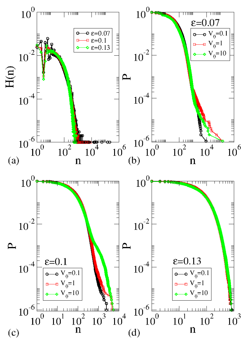
The histogram of frequency for the escaping orbits is shown in Fig. 6(a) for the parameters $p=3$, $a=0.1$ and the same three different $\epsilon$, as used in the static case. We can see from the histogram (Fig. 6(a)) that the escaping particles at 3 collisions are still less observed than the ones for 2 and 4 collisions. The survival probability was considered for different values of $\epsilon$ and for three different values of initial velocity. For $\epsilon=0.07$, we can see in Fig. 6(b) that the survival probability decays exponentially fast and few orbits keep trapped at large $n$ therefore leading the curve to slower the decay at the end. The slower initial velocity $V_{0}=0.1$ seems to affect less the dynamics while a short tail of slower decay is observed for $V_{0}=1$ and $V_{0}=10$. For $\epsilon=0.1$ (see Fig. 6(c)), the survival probability for $V_{0}=10$ is marked by a hump starting at $n\approx 400$ while few orbits are trapped in sticky domain for $V_{0}=1$ and $V_{0}=0.1$. On the other hand, when $\epsilon=0.13$ (see Fig. 6(d)), no significant changes from fast exponential decay was observed as dependent on the initial velocity.

Let us discuss the results obtained for the survival probability considering the two cases of (i) static and (ii) time-varying boundary. For the static boundary, the velocity of the particle is constant and for a mixed phase space where invariant spanning curves and KAM islands coexist, the sticky behavior observed is larger as compared to the case where invariant spanning curves are destroyed ($\epsilon\geq\epsilon_{c}$ (see Ref. [19])) and chaotic sea is limited by KAM islands only. Therefore the decay of the survival probability starts exponentially at short collisions and suddenly it is marked by a changeover turning into a power law for large number of collisions. On the other hand, when the invariant spanning curves are destroyed but the period three region in the phase space still influences the dynamics, several instances of trapping were observed leading the dynamics to spend long time near period three orbits. The decay of the survival probability starts exponentially fast at short collisions and suddenly it changes to a slower decay being characterized by a stretched exponential. The decay is slower than exponential but is still faster than a power law. Indeed, as the control parameters are varied and invariant spanning curves are destroyed, one can observe a continuum spectrum of decay ranging from exponential to a power law. This variation is still an open problem and extensive theoretical and numerical investigations should be made to describe it properly. As the parameter $\epsilon$ rises, the elliptic region in the phase space decreases and the exponentially fast decay of the survival probability is most evident. However trapping is still observed for large times. In our case we observed a few long orbits trapped near a region of period twelve. Such orbits indeed slow the decay of the survival probability at the very long time but were observed only in a few trajectories.

For case (ii) where a time varying boundary is considered, the velocity of the particle is no longer constant. The LRA conjecture claims [37], the chaotic dynamics of the particle for the static boundary leads to the unlimited energy growth when a time perturbation is considered; numerical studies of this model are consistent with this prediction [46, 51]. A consequence is that a particle with high energy collides many more times with the boundary in a given interval of time while compared with a lower energy particle at the same interval of time. Over a small number of collisions the billiard it sees is effectively static, and it is likely to escape well before Fermi acceleration is evident. This is observed particularly for the case of $\epsilon=0.1$ and $V_{0}=10$ where a hump in the survival probability is evident.

4 Concluding remarks

We have studied some dynamical properties of an oval-like billiard with a hole in the boundary, considering both static as well as time dependent boundaries. For the static case, the recurrence time distribution of the hole has a fast decay for short collisions changing the decay either to a power law or stretched exponential, depending on the control parameter. The power law observed for $\epsilon=0.07$ in the static case has slope $-2.431(4)$ while the stretched exponential for $\epsilon=0.1$ is given by $P=P_{0}\exp(b~{}n^{\gamma})$ with coefficients $P_{0}=0.0054$, $b=-0.104$ and $\gamma=0.47$. The sticky orbits present in the dynamics are responsible for slowing the decay of the recurrence time distribution. For the time dependent case, the survival probability was considered for different values of $\epsilon$ and for three different values of initial velocity. For $\epsilon=0.07$, the lower initial velocity seems to affect less the trapping orbits while a short tail is observed for larger initial velocities indicating a sticky regime. For $\epsilon=0.1$, the initial $V_{0}=10$ lead the survival probability to exhibit a hump starting at $n\approx 400$ therefore indicating a sticky regime. Indeed at that large energy, the particle suffers many more collisions with the boundary at the same interval of time as compared to a low energy particle, hence seeing less the influence of the moving boundary compared with a lower energy particle, therefore seem to be more susceptible to sticky behavior. For $\epsilon=0.13$ the initial velocities considered do not seem to change significantly the fast exponential decay as observed for $\epsilon=0.1$ and $\epsilon=0.07$.

The observation of stretched exponential decays, as in Ref. [50], invites further investigation, as previous studies have concentrated on algebraic decay models. We would like to remark that as in Ref. [50], a stretched exponential decay is observed where there is a single prominent elliptic periodic orbit responsible for the stickiness, and also that the exponent $\gamma$ is very close to $1/2$. In general, opening a dynamical system with a hole is a very effective method of elucidating the structure of intermittent dynamics.

References

- [1] N. Chernov, R. Markarian, Chaotic Billiards (American Mathematical Society, 2006).
- [2] S. Tabachnikov, Geometry and billiards (American Mathematical Society, 2005).
- [3] D. Sweet et al., Physica (Amsterdam) 154D, 207 (2001).
- [4] H. D. Graf et al., Phys. Rev. Lett. 69, 1296 (1992).
- [5] T. Sakamoto et al., Jpn. J. Appl. Phys. 30, L1186 (1991).
- [6] J. P. Bird, J. Phys. Condens. Matter 11, R413 (1999).
- [7] E. Persson et al., Phys. Rev. Lett. 85, 2478 (2000).
- [8] J. Stein, H. J. Stokmann, Phys. Rev. Lett. 68, 2867 (1992).
- [9] H. J. Stokmann, Quantum Chaos: An Introduction (Cambridge University Press - 1999).
- [10] V. Milner et al., Phys. Rev. Lett. 86, 1514 (2001).
- [11] N. Friedman et al., Phys. Rev. Lett. 86, 1518 (2001).
- [12] M. F. Andersen et al., Phys. Rev. A, 69, 63413 (2004).
- [13] M. F. Andersen et al., Phys. Rev. Lett. 97, 104102 (2006).
- [14] C. M. Marcus et al., Phys. Rev. Lett. 69, 506 (1992).
- [15] M. V. Berry, Eur. J. Phys. 2, 91, (1981).
- [16] L. A. Bunimovich, Commun. Math. Phys. 65, 295, (1979).
- [17] V. Lopac, I. Mrkonjic, N. Pavin et. al., Physica D 217, 88 (2006).
- [18] V. Lopac, I. Mrkonjic, D. Radic, Phys. Rev. E 64, 016214 (2001).
- [19] D. F. M. Oliveira, E. D. Leonel, Commun Nonlinear Sci Numer Simulat 15 1092, (2010).
- [20] M. Robnik, Prog. Theor. Phys. Sup 150, 229 (2003).
- [21] Y. G. Sinai, Russ. Math. Surveys, 25, 137 (1970); 25, 141 (1970).
- [22] L. A. Bunimovich and C. P. Dettmann, EPL 80, 40001 (2007).
- [23] “Hard ball systems and the Lorentz gas” Ed. D. Szasz, (Springer, 2000).
- [24] D. F. M. Oliveira, J. Vollmer, Edson D. Leonel, Physica D, 240, 389 (2011).
- [25] L. A. Bunimovich and A. Grigo, Commun. Math. Phys. 293, 127 (2010).
- [26] C. P. Dettmann, J. Stat. Phys. (to appear); arxiv:1103.1225.
- [27] J. Marklof and A. Strombergsson, GAFA Geometric and Functional Analysis 21, 560 (2011).
- [28] L. A. Bunimovich, Chaos 11, 802 (2001).
- [29] C. P. Dettmann, O. Georgiou, J. Phys. A 44, 195102 (2011).
- [30] A. Loskutov, Phys. Usp. 50, 939 (2007).
- [31] E. Fermi, Phys. Rev. 75, 1169 (1949).
- [32] A. Y. Loskutov, A. B. Ryabov, and L. G. Akinshin, J. Exp. Theor. Phys. 89, 966 (1999).
- [33] P. J. Holmes, J. Sound Vib. 84, 173 1982.
- [34] A. K. Karlis, P. K. Papachristou, F. K. Diakonos, V. Constantoudis, and P. Schmelcher, Phys. Rev. Lett. 97, 194102 (2006); Phys. Rev. E 76, 016214 (2007).
- [35] A. J. Lichtenberg and M. A. Lieberman, Regular and Chaotic Dynamics, Applied Mathematical Sciences Vol. 38, (Springer-Verlag, New York, 1992).
- [36] D. G. Ladeira and Jafferson Kamphorst Leal da Silva, Phys. Rev. E 73, 026201 (2006).
- [37] A. Loskutov, A. B. Ryabov, L. G. Akinshin, J. Phys. A 33, 7973 (2000).
- [38] F. Lenz, F. K. Diakonos, P. Schmelcher, Phys. Rev. Lett. 100, 014103 (2008).
- [39] E. D. Leonel, L. A. Bunimovich, Phys. Rev. Lett. 104, 224101 (2010).
- [40] K. Shah, D. Turaev, V. Rom-Kedar, Phys. Rev. E 81, 056205 (2010).
- [41] B. Liebchen, R. Buchner, C. Petri, F. K. Diakonos, F. Lenz, P. Schmelcher, New J. Phys. 13 093039, (2011).
- [42] E. D. Leonel, J. A. de Oliveira, F. Saif, J. Phys. A: Math. Theor. 44, 302011 (2011).
- [43] E. G. Altmann, A. E. Motter, H. Kantz, Phys. Rev. E 73, 026207 (2006).
- [44] E. G. Altmann, E. C. da Silva, I. L. Caldas, Chaos 14, 975 (2004).
- [45] D. R. da Costa, D. P. Dettmann, E. D. Leonel, Phys. Rev. E 83, 066211 (2011).
- [46] E. D. Leonel, D. F. M. Oliveira and A. Loskutov, Chaos 19, 033142 (2009).
- [47] M. M. A. Sieber, J. Phys. A 30, 4563 (1997).
- [48] J. U. Nöckel, A. D. Stone, G. Chen, H. L. Grossman and R. K. Chang, Opt. Lett. 21, 1609 (1996).
- [49] A. Arroyo, R. Markarian, D. P. Sanders, Nonlinearity 22, 1499 (2009).
- [50] C. P. Dettmann, E. D. Leonel, Physica D, 241, 403 (2012).
- [51] D. F. M. Oliveira, E. D. Leonel, Physica A 389, 1009 (2010).