Optimal control for non-Markovian open quantum systems

Abstract

An efficient optimal control theory based on the Krotov method is introduced for a non-Markovian open quantum system with a time-nonlocal master equation in which the control parameter and the bath correlation function are correlated. This optimal control method is developed via a quantum dissipation formulation that transforms the time-nonlocal master equation to a set of coupled linear time-local equations of motion in an extended auxiliary Liouville space. As an illustration, the optimal control method is applied to find the control sequences for high-fidelity $Z$-gates and identity-gates of a qubit embedded in a non-Markovian bath. $Z$-gates and identity-gates with errors less than $10^{-5}$ for a wide range of bath decoherence parameters can be achieved for the non-Markovian open qubit system with control over only the $\sigma_{z}$ term. The control-dissipation correlation, and the memory effect of the bath are crucial in achieving the high-fidelity gates.

I Introduction

Quantum optimal control theory (QOCT) Rabitz88 ; Tannor92 ; Kosloff02 ; Montangero2007 ; Nielsen08 ; Khaneja05 ; Tannor11 is a powerful tool that provides a variational framework for calculating the optimal shaped pulse to maximize a desired physical objective (or minimize a physical cost function). It has been applied to various open quantum systems or models to obtain control sequences for quantum gate operations Rebentrost2009 ; potz2008 ; potz2009 ; Jirari2009 ; Gordon08 ; Clausen10 . Compared to the dynamical-decoupling-based method West10 in which a succession of short and strong pulses designed to suppress decoherence is applied to the system, QOCT is a continuous dynamical modulation with many degrees of freedom for selecting arbitrary shapes, durations and strengths for time-dependent control, and thus allows significant reduction of the applied control energy and the corresponding quantum gate error. The authors of Ref. Rebentrost2009 investigated the optimal control of a qubit coupled to a two-level system that is exposed to a Markovian heat bath. Although this may mimic the reduced non-Markovian dynamics of the qubit, it is by no means a model of a qubit coupled directly to a non-Markovian environment. The authors of Refs. potz2008 ; potz2009 ; Jirari2009 investigated optimal quantum gate operations in the presence of non-Markovian environments. However, to combine QOCT with a non-Markovian master equation involving time-ordered integration of the nonunitary (dissipation) terms for noncommuting system and control operators, and for a nonlocal-in-time memory kernel, the numerical treatment is rather mathematically involved and computationally demanding. All of the QOCT approaches mentioned above Rebentrost2009 ; potz2008 ; potz2009 ; Jirari2009 ; Gordon08 ; Clausen10 for open quantum systems employed gradient-based Rabitz88 ; Khaneja05 algorithms for optimization.

A somewhat different QOCT approach from the standard gradient optimization methods is the Krotov iterative method krotov1996 ; Tannor92 ; Nielsen08 ; Tannor11 . The Krotov method has several appealing advantages Tannor92 ; Nielsen08 ; Tannor11 over the gradient methods: (a) monotonic increase of the objective with iteration number, (b) no requirement for a line search, and (c) macrosteps at each iteration. A version of the Krotov optimization method has been used recently in Ref. Schmidt11 to deal with the non-Markovian optimal control problem of a quantum Brownian motion model with an exact stochastic equation of motion (master equation). We note however that only a few non-Markovian open quantum system models are exactly solvable Schmidt11 ; Breuer02 ; Hu92 ; Diosi98 ; Strunz04 ; Yan09 ; Chang10 ; Yu10 (the quantum Brownian model is one of them), and the exact master equations of these exactly solvable models are known to be in a time-local (time-convolutionless) form with time-dependent decoherence or decay rates, without involving the time-ordering problem of non-commuting operators. Schmidt11 ; Breuer02 ; Hu92 ; Diosi98 ; Strunz04 ; Yan09 ; Chang10 ; Yu10 . With time-local equations of motion, the Krotov method could be directly employed to deal with optimal-control problems. Although it is commendable to derive an exact master equation, not too many problems can be exactly worked out in this way. For example, no exact master equation can be derived for the non-Markovian qubit-environment (spin-boson) model studied as an illustration for quantum gate operations in this paper. It is thus important that an efficient QOCT approach based on the Krotov method for perturbative treatment of general (not limited to just some certain classes of) non-Markovian open quantum systems should be developed. The perturbative non-Markovian master equation under only the Born approximation (or the weak system-bath coupling approximation) Breuer02 is in the form of a time-ordered non-commuting integro-differential equation [e.g., see Eqs. (1) and (2)], and at first sight it is not at all clear how to effectively combine this kind of master equation with the Krotov optimization method. The study presented in this paper provides just such an efficient QOCT approach based on the Krotov method to deal with time-nonlocal non-Markovian open quantum systems. Our approach transforms the time-ordered non-commuting integro-differential master equation into a set of time-local coupled differential equations with the small price of introducing auxiliary density matrices in an extended auxiliary Liouville space. As a result, incorporation of the resultant time-local equations with the Krotov optimization method becomes effective. We then apply the developed Krotov method to the problem of finding the optimal quantum gate control sequence for a qubit in a non-Markovian environment (bath). Our results illustrate that the control parameter can be engineered to efficiently counteract and suppress the environment effect for non-Markovian open systems with long bath correlation times (long memory effects). We also find that high-fidelity quantum gates with error smaller than $10^{-5}$ can be achieved at long gate operation times for a wide range of bath decoherence parameters. This is in contrast to the cases in the literature Rebentrost2009 ; potz2008 ; potz2009 ; Jirari2009 , where the non-Markovian systems were mainly studied in a parameter regime very close to Markovian systems, and thus no significant reduction of the quantum gate errors was observed.

II Non-Markovian master equation and quantum optimal control theory

In realistic experiments, one may have only limited control over the system Hamiltonian, and the maximum control parameter strength that can be realized is also restricted. Let us consider a total system with Hamiltonian $H=H_{S}(t)+H_{I}+H_{B}$. Here the system Hamiltonian $H_{S}(t)=-\hbar\varepsilon(t)\sigma_{z}/2-\hbar\Omega\sigma_{x}/2$, describes a qubit with a time-dependent control parameter $\varepsilon(t)$ and a fixed tunneling frequency $\Omega$, i.e., having control over only the $\sigma_{z}$ term. The bath Hamiltonian is $H_{B}=\sum_{q}\hbar\omega_{q}{b_{q}}^{\dagger}b_{q}$, where ${b_{q}}^{\dagger}$ (${b_{q}}$) is the creation (annihilation) operator of the bath mode $q$ with frequency $\omega_{q}$. The interaction Hamiltonian $H_{I}$ between the system and the bath without making the rotating-wave approximation is of the form $H_{I}=\sigma_{x}\sum_{q}c_{q}(b_{q}+{b_{q}}^{\dagger})$, where $c_{q}$ is the coupling constant of bath mode $q$ to the qubit system. Following the standard perturbation theory, we obtain (see the Appendix A for the derivation) under only the Born approximation the time-convolution master equation for the reduced system density matrix as Meier99 ; Yan01 ; Kleinekathofer04 ; Kleinekathofer06

$$\dot{\rho}(t)=\mathcal{L}_{S}(t)\rho(t)+\{\mathcal{L}_{x}\mathcal{K}(t)+[\mathcal{L}_{x}\mathcal{K}(t)]^{\dagger}\}.$$ (1)

Here the superoperators $\mathcal{L}_{S}(t)$ and $\mathcal{L}_{x}$ are defined via their actions on an arbitrary operator $A$, respectively, as $\mathcal{L}_{S}(t)A=\frac{1}{i\hbar}[H_{S}(t),A]$ and $\mathcal{L}_{x}A=\frac{1}{i\hbar}[\sigma_{x},A]$. The non-Hermitian (dissipation) operator can be written as

$$\mathcal{K}(t)=\frac{1}{i\hbar}\int_{0}^{t}dt^{\prime}C(t-t^{\prime})\mathcal{U}_{S}(t,t^{\prime})\sigma_{x}\rho(t^{\prime}),$$ (2)

where the unitary qubit system propagator superoperator $\mathcal{U}_{S}(t,t^{\prime})=T_{+}\exp\{\int^{t}_{t^{\prime}}d\tau\mathcal{L}_{S}(\tau)\}$ with $T_{+}$ being the time-ordering operator, and the bath correlation function (CF) is $C(t-t^{\prime})=\int_{0}^{\infty}d\omega J(\omega)\cos[\omega(t-t^{\prime})]\coth[{\hbar\omega}/({2k_{B}T})]-i\int_{0}^{\infty}d\omega J(\omega)\sin[\omega(t-t^{\prime})]$ with $T$ being the temperature. Note that Eq. (2) contains the bath CF $C(t,t^{\prime})$ and the time-ordered system propagator superoperator $\mathcal{U}_{S}(t,t^{\prime})$ which involves the control parameter $\varepsilon(t)$ through $H_{S}(t)$ in $\mathcal{L}_{S}(t)$. Thus the control parameter and bath-induced nonunitary (dissipation) effect are correlated. This paves the way for manipulating the control sequence to counteract the effect of the bath on the system dynamics. This coherent control of non-Markovian open quantum systems is in contrast to various Markovian approaches of engineering reservoirs ER and incoherent controls by directly manipulating the environments ICE .

In the framework of the QOCT, one would like to maximize the quality (fidelity) value of some target at time $t_{f}$. Suppose the desired state-independent unitary quantum gate operation is denoted as $\mathcal{O}$ and the target is to perform a state-independent quantum gate operation as close as possible to $\mathcal{O}$. We choose the trace distance between the desired target superoperator $\mathcal{O}$ and the actual nonunitary propagator superoperator $\mathcal{X}(t_{f})$ at the final operation time $t_{f}$ to characterize the gate error, i.e., $\text{(error)}=\text{Tr}\{[\mathcal{O}-\mathcal{X}(t_{f})]^{2}\}/N$, where $N$ is the dimension value of $\mathcal{O}$. As minimizing the trace distance is similar to maximizing the real part of the trace fidelity Rebentrost2009 , we choose $\mathcal{F}={\rm Re}[\text{Tr}\{\mathcal{O}^{\dagger}\mathcal{X}(t_{f})\}]/N$ as a quality (fidelity) measure of how well $\mathcal{X}(t_{f})$ approaches the target $\mathcal{O}$ in the QOCT framework. In realistic control problems, it is desirable that the optimal control sequence can provide highest quality (fidelity) with minimum energy consumption. Thus we introduce an objective function of the form

$$\mathcal{J}=\mathcal{F}-\int_{0}^{t_{f}}dt^{\prime}\lambda(t^{\prime})[\varepsilon(t^{\prime})-\varepsilon_{0}(t^{\prime})]^{2},$$ (3)

where $\lambda(t)$ is a positive function that can be adjusted and chosen empirically, $\varepsilon(t)$ is the control parameter and $\varepsilon_{0}(t)$ is a reference control value that can be properly chosen Tannor92 ; Kosloff02 . Then the task of quantum control is to maximize the objective (3) under the constraint of the equation of motion of $\mathcal{X}(t)$ obtained by replacing $\rho(t)$ with $\mathcal{X}(t)$ in Eqs. (1) and (2).

The time-dependent control parameter $\varepsilon(t)$ enters into the exponent of the time-ordered system propagator $\mathcal{U}_{S}(t,t^{\prime})$, and thus appears inside the memory kernel or dissipation operator Eq. (2). As a result, Eq. (1) is a nonlocal time-ordered integro-differential equation in which values of the control parameter at all earlier times come into play, and is difficult to incorporate within the framework of QOCT. Thus an approach that retains the merits of the Krotov optimization method and removes the time-ordering and nonlocal problems in the equation of motion is very much desired.

III Master equation and optimal control in extended Liouville space

One important observation to deal with the time-nonlocal non-Markovian quantum master equation is to express the bath CF’s in a multi-exponential form Meier99 ; Yan01 ; Kleinekathofer04 ; Kleinekathofer06 , $C(t-t^{\prime})=\sum_{j}C_{j}(0)e^{\gamma_{j}(t-t^{\prime})}$, where $C_{j}(0)$ and $\gamma_{j}$ are complex constants and can be found by numerical methods. Then Eq. (2) can be written as $\mathcal{K}(t)=\sum_{j}\mathcal{K}_{j}(t)$, where $\mathcal{K}_{j}(t)=\frac{1}{i\hbar}\int_{0}^{t}dt^{\prime}C_{j}(0)e^{\gamma_{j}(t-t^{\prime})}\mathcal{U}_{S}(t-t^{\prime})\sigma_{x}\rho(t^{\prime})$. Although $\mathcal{K}_{j}(t)$ is still a time-nonlocal and time-ordered integration for non-commuting operators, if one takes the time derivative of $\mathcal{K}_{j}(t)$, one obtains

$$\dot{\mathcal{K}}_{j}(t)=({1}/{i\hbar})C_{j}(0)\sigma_{x}\rho(t)+[\mathcal{L}_{S}(t)+\gamma_{j}]\mathcal{K}_{j}(t),$$ (4)

with initial condition $\mathcal{K}_{j}(0)=0$. The same process can be done for the Hermitian conjugate ${\mathcal{K}}^{\dagger}(t)\equiv\sum_{j}{\mathcal{K}_{j}}^{\dagger}(t)$. Equation (1) combined with Eq. (4) and its Hermitian conjugate form a set of coupled linear equations of motion that can be written as $\dot{\vec{\rho}}(t)=\hat{\Lambda}(t)\vec{\rho}(t)$, in terms of $\vec{\rho}(t)\equiv\{\rho(t),\mathcal{K}_{j},{\mathcal{K}_{j}}^{\dagger};j=1,2,3,...\}$ in an extended auxiliary Liouville space Meier99 ; Yan01 ; Kleinekathofer04 ; Kleinekathofer06 . Obviously, the above equations are time-local and have no time-ordering and memory kernel integration problems. This yields a simple, fast and stable iterative scheme to incorporate with the Krotov method. The formal solution of $\vec{\rho}(t)$ can be written as $\vec{\rho}(t)=\hat{\mathcal{G}}(t)\vec{\rho}(0)$, where the associated propagator superoperator can be shown to satisfy $[{\partial\hat{\mathcal{G}}(t)}/{\partial t}]=\hat{\Lambda}(t)\hat{\mathcal{G}}(t)$ with $\hat{\mathcal{G}}(0)=\hat{{I}}_{\mathcal{N}}$. Here $\hat{{I}}_{\mathcal{N}}$ is the identity operator in the extended Liouville space and $\mathcal{N}$ is the dimension of $\hat{\mathcal{G}}(t)$. The real part of the trace fidelity for the propagator $\hat{\mathcal{G}}(t_{f})$ is $\mathcal{F}={\rm Re}[\text{Tr}\{\hat{\mathcal{Q}}^{\dagger}\hat{\mathcal{G}}(t_{f})\}]/\mathcal{N}$, where $\hat{\mathcal{Q}}$ is the target operator $\mathcal{O}$ in the extended Liouville space. The goal of quantum optimal control here is to reach a desired target $\hat{\mathcal{Q}}$ with maximum objective function $\mathcal{J}$ (or fidelity $\mathcal{F}$) in a certain time $t_{f}$. The optimal algorithm following the Krotov method krotov1996 is summarized as follows Tannor92 ; Kosloff02 ; Nielsen08 . (i) Guess an initial control sequence $\varepsilon_{0}(t)$. (ii) Use the equations of motion to find the forward propagator $\hat{\mathcal{G}}_{k}(t)$ with the initial condition $\hat{\mathcal{G}}(0)=\hat{{I}}_{\mathcal{N}}$ ($k=0$ for the first iteration). (iii) Find an auxiliary backward propagator $\hat{\mathcal{B}}_{k}(t)$ with the condition $\hat{\mathcal{B}}(t_{f})=\hat{\mathcal{Q}}^{\dagger}$. (iv) Propagate $\hat{\mathcal{G}}_{k+1}(t)$ again forward in time, and update the control parameter iteratively with the rule $\varepsilon_{k+1}(t)=\varepsilon_{k}(t)+\frac{1}{2\lambda(t)}\text{Re}[\text{Tr}\{\hat{\mathcal{B}}_{k}(t)\frac{\partial\Lambda(t)}{\partial\varepsilon(t)}\hat{\mathcal{G}}_{k+1}(t)\}].$ (v) Repeat steps (iii) and (iv) until a preset fidelity (error) is reached or until a given number of iterations has been performed.

IV Results and discussions

To find the optimal control sequence for a state-independent single-qubit gates in a non-Markovian bath, one needs to know the bath spectral density to calculate the bath CF. We can deal with any form of the bath spectral density, but for simplicity, we take an Ohmic spectral density in the form of $J(\omega)=\alpha\omega e^{-\omega/\omega_{c}}$, where $\alpha$ is a dimensionless damping constant, and $\omega_{c}$ is the bath cutoff frequency. The bath CF can thus be calculated and can then be expanded directly in a multi-exponential form. The values of $C_{j}(0)$ and $\gamma_{j}$ of the exponentials are obtained numerically with the requirement that the error between the actual CF and the approximated CF is chosen to be less than or equal to $10^{-7}$. Only three or four exponential terms in the expansion are required to express the bath CF with such high accuracy as compared to a sum of more than 48 exponentials needed to express the same bath CF at a low temperature of $T=0.2\Omega$ through the spectral density parametrization Meier99 . We note here that both the parametrization of Ref. Meier99 , which is highly efficient at moderate to high temperatures, and the direct bath CF decomposition of our approach are well-suited for the parametrization of highly structured spectral densities, leading to long and oscillatory bath CF’s. However, our approach has a great computational advantage over the commonly used approach of spectral density parametrization Meier99 ; Yan01 ; Kleinekathofer04 ; Kleinekathofer06 at low temperatures.

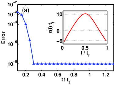
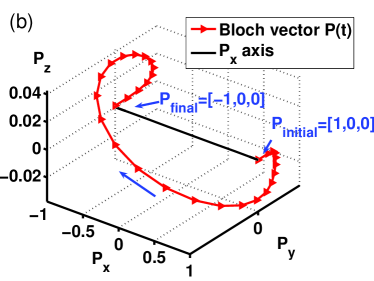
Figure 1: (Color online) (a) Unitary $Z$-gate error versus operation time $t_{f}$. (b) Bloch vector trajectory of an optimal unitary $Z$-gate operation with the initial polarization condition $P(0)=[1,0,0]$. The inset in (a) is the optimal control pulse sequence for any $t_{f}\geq 0.3\Omega$.

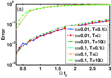
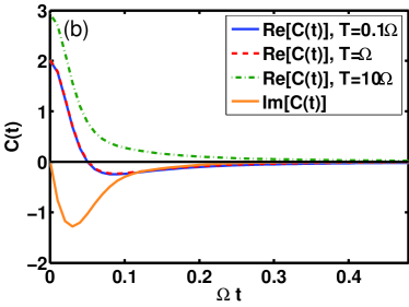
Figure 2: (color online) (a) Z-gate error versus time $t_{f}$ for different values of $\alpha$ and $T$ at $\omega_{c}=20\Omega$. The stopping criterion of the error threshold is set to $10^{-6}$ or when the number of iterations exceeds $3000$. (b) Corresponding bath CF’s for $\alpha=0.01$. We set $k_{B}=1$ and $\hbar=1$ in all the figures presented here and below.

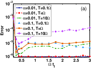
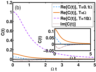
Figure 3: (Color online) (a) $Z$-gate error versus time $t_{f}$ for the same bath parameters and stopping criterion as in Fig. 2 except $\omega_{c}=\Omega$. (b) Corresponding bath CF’s for $\alpha=0.1$. The lower three curves are plotted in a smaller vertical-axis range in the inset.

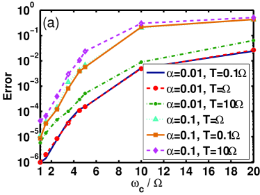
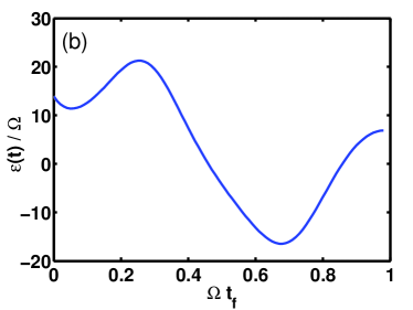
Figure 4: (Color online) (a) $Z$-gate error versus cutoff $\omega_{c}$ for different values of $\alpha$ and $T$ with $t_{f}=\Omega^{-1}$. (b) Optimal $Z$-gate control sequence for $\alpha=0.01$, $T=\Omega$, $t_{f}=\Omega^{-1}$ and $\omega_{c}=\Omega$.

The ideal $Z$-gate performance as a function of the gate operation time $t_{f}$ in the absence of the bath is given in Fig. 1 with the stopping criterion of error set to $10^{-8}$. For all the calculations performed in this paper, we restrict the maximum control parameter $\varepsilon(t)\leq 30\Omega$. Excellent $Z$-gate performance can be achieved for pulse time $t_{f}\geq 0.3/\Omega$. The corresponding optimal pulse sequence is shown in the inset of Fig. 1(a). In fact, a unitary $Z$-gate for pulse time $t_{f}>0.3/\Omega$ with error limited only by machine precision can be achieved. Furthermore, if one does not impose any restriction on the maximum control parameter strength, an optimal perfect $Z$-gate can be achieved for any finite period of time $t_{f}$. This is in contrast to the control pulse strategy for the implementation of a (unitary) $Z$-gate in Rebentrost2009 , where the gate operation time $t_{f}\geq\pi/\Omega$, corresponding to the static $\Omega\sigma_{x}$ inducing at least a full loop around the $x$ axis. One can see from the Bloch polarization vector evolution in Fig. 1(b) that our optimal control pulse strategy does not require a full loop around the $x$ axis as compared with the state evolution in Fig. 2 (left panel) of Rebentrost2009 , and thus can achieve a $Z$-gate in a much shorter operation time limited primarily by the control parameter strength.

Figures 2 and 3 show the errors of the $Z$-gate versus operation times and the corresponding bath CF’s for different values of the bath dimensionless damping constant $\alpha$ and temperature $T$ at cutoff frequencies $\omega_{c}=20\Omega$ and $\omega_{c}=\Omega$, respectively. Note that the imaginary part of the bath CF does not depend on temperature $T$, so only one curve of the imaginary part is plotted in Figs. 2(b) and 3(b). One can see that for $\omega_{c}=20\Omega$, the gate errors increase with the operation times $t_{f}$ for all the different bath parameter cases studied in Fig. 2(a). The errors for the case of smaller $\alpha=0.01$ are about $10^{-3}$ at the beginning and increase to $10^{-1}$ at longer operation times. As expected, the gate performance deteriorates as the value of $\alpha$ increases. The value of $\alpha$ plays a more important role than that of temperature in determining the amount of the error for the $\omega_{c}=20\Omega$ case. The bath CF at time $t=0$ for the high-temperature case of $k_{B}T=10\hbar\Omega$ is bigger than that for the low temperature case of $k_{B}T=\hbar\Omega$ by a factor of only $1.5$ as shown in Fig. 2(b). However, the bath CF (effective decay rate) is directly proportional to $\alpha$. Therefore, the gate errors for the case $\omega_{c}=20\Omega$ shown in Fig. 2(a) depend mainly on the value of $\alpha$. In all the previous investigations of quantum gate performance for both Markovian and non-Markovian open quantum systems Rebentrost2009 ; potz2008 ; potz2009 ; Jirari2009 , the gate errors for a value of $\alpha=0.01$ are about $10^{-3}$ or worse. This is similar to what we found for the $\omega_{c}=20\Omega$ case. However, one of our main results, significantly different from previous investigations, is that for small $\omega_{c}$, it is possible to achieve high-fidelity $Z$-gates with errors smaller than $10^{-5}$ at large times, as shown in Fig. 3(a). This can be understood from the control-dissipation correlation, Eq. (2), and the memory effect of the non-Markovian environment. The bath CF’s in Figs. 3(a) and 2(a) decay to zero on a time scale of $t_{B}\approx\omega_{c}^{-1}$, called the bath correlation time. For $\omega_{c}=20\Omega$, the bath is very close to Markovian, and the dissipator (2) or decay rate approaches a constant value in a very short time of $t_{B}\approx 0.05\Omega^{-1}$ and thus cannot be significantly suppressed by the external control sequence. On the other hand, for $\omega_{c}=\Omega$, the longer bath correlation time of $t_{B}\approx\Omega^{-1}$ allows the optimal control sequence to have enough action time to counteract and suppress the contribution from the bath in the weak system-bath coupling case, and thus reduces the gate error considerably. For $\alpha=0.01$ and temperature $k_{B}T\leq\hbar\Omega$, the gate error can be kept about or smaller than $10^{-6}$. The temperature $T$ plays a similar role to the coupling strength when $k_{B}T>\hbar\Omega$, as the amplitude ratio of the bath CF between the $k_{B}T=10\hbar\Omega$ and $k_{B}T\leq\hbar\Omega$ cases is about $10$. Even though the gate errors for larger $\alpha$ and higher $T$ increase with $t_{f}$, the errors for all of the cases studied except for the case of $\alpha=0.1$ and $T=10\Omega$ in Fig. 3(a) are smaller than $10^{-5}$, smaller than the error threshold of $10^{-4}$ ($10^{-3}$) Preskill09 required for fault-tolerant quantum computation. We also perform calculations for an optimal identity gate and the behaviors of the gate errors versus operation times $t_{f}$ are similar to that of the $Z$-gate in Fig. 3(a). Achieving a high-fidelity identity gate at long times implies having the capability for arbitrary state preservation, i.e., storing arbitrary state robustly against the bath. The gate errors are expected to be much lower if one has independent control over both the $\sigma_{z}$ and $\sigma_{x}$ terms in the qubit Hamiltonian and if there is no restriction on the control parameter strengths.

Figure 4(a) shows the Z-gate error versus bath cutoff frequency $\omega_{c}$ at operation time $t_{f}=\Omega^{-1}$ for different values of $\alpha$ and $T$. One can see that the gate error depends strongly on the bath cutoff frequency. The error increases as $\omega_{c}$ becomes bigger. For the weak coupling and low temperature cases ($\alpha=0.01$, $T\leq\Omega$), it is possible to reduce the error to below $10^{-5}$ for $\omega_{c}\leq 2.5\Omega$. These indicate that the bath correlation time $t_{B}\approx\omega_{c}^{-1}$ or memory effect plays an important role in determining the gate error. Figure 4(b) shows the optimal control sequence for $\omega_{c}=\Omega$, $\alpha=0.01$, $k_{B}T=\hbar\Omega$ and $t_{f}=\Omega^{-1}$. The optimal control sequence that suppresses the decoherence induced by the bath is totally different from that of the ideal unitary case in the inset of Fig. 1(a).

V Conclusion

To conclude, a universal QOCT based on the Krotov method for a time-nonlocal non-Markovian open quantum system has been introduced and applied to obtain control sequences and gate errors for $Z$ and identity gates. Our study has yielded several computational and conceptual innovations: (a) The QOCT that combines the Krotov method and an extended Liouville space quantum dissipation formulation that transforms the nonlocal-in-time master equation to a set of coupled linear local-in-time equations of motion is introduced to deal with non-Markovian open quantum systems. (b) The direct numerical decomposition of the bath CF into multi-exponential form has a great computational advantage over the commonly used spectral density parametrization approach Meier99 ; Yan01 ; Kleinekathofer04 ; Kleinekathofer06 . (c) The constructed QOCT, which retains the merits of the Krotov method, is extremely efficient in dealing with the time-nonlocal non-Markovian equation of motion. Compared to the calculations performed on a 40-node SUN Linux cluster via the gradient-based approach to tackle the nonlocal kernel directly potz2008 , the calculations using our approach for a similar problem can be performed on a typical laptop PC with ease, thus opening the way for investigating two-qubit and many-qubit problems in non-Markovian environments. (d) Our study of optimal control reveals the strong dependence of the gate errors on the bath correlation time and exploits this non-Markovian memory effect for high-fidelity quantum gate implementation and arbitrary state preservation in an open quantum system. The presented QOCT has been shown to be a powerful tool, capable of facilitating implementations of various quantum information tasks against decoherence. The required information is knowledge of the bath or noise spectral density which is experimentally accessible by, for example, dynamical decoupling noise spectroscopy techniques Yuge11 ; Suter11 ; Bylander11 ; Almog11 ; Biercuk11 . We note here that not only our proposed method of QOCT but also dynamical decoupling and other strategies for fighting decoherence require knowledge of the spectral distribution of the noise (bath spectral density) in order to improve the strategies and design effective and/or optimized control sequences Suter07 ; Uhrig08 ; Biercuk09 ; Uys09 ; Gordon08 ; Clausen10 . Thus using the dynamical decoupling noise spectroscopy techniques Yuge11 ; Suter11 ; Bylander11 ; Almog11 ; Biercuk11 to determine the bath spectral densities experienced by the qubits and then applying QOCT to find explicitly control sequences for quantum gate operations for the non-Markovian open qubit system will yield fast quantum gates with low invested energy and high fidelity . By virtue of its generality and efficiency, our Krotov based QOCT method will find useful applications in many different branches of the sciences. Recent experiments on engineering external environments Wineland00 , simulating open quantum systems Blatt11 , and observing non-Markovian dynamics Madsen11 ; Liu could facilitate the experimental realization of the QOCT in non-Markovian open quantum systems in the near future.

*

Appendix A Derivation of the time-nonlocal master equation

Here we provide the derivation of the time-nonlocal non-Markovian master equation (1) and (2) in the text. Following the assumption of factorized initial system-bath state $\rho_{T}(0)=\tilde{\rho}_{T}(0)=\rho(0)\otimes R_{0}$, the standard perturbative time-convolution (under only the Born approximation) master equation in the interaction picture takes the form of

$$\dot{\tilde{\rho}}(t) = -\frac{i}{\hbar}{\rm Tr}_{B}[\tilde{H}_{I}(t),\rho(0)\otimes R_{0}]$$ (5)

$$-\frac{1}{\hbar^{2}}{\rm Tr}_{B}\int_{0}^{t}dt^{\prime}[\tilde{H}_{I}(t),[\tilde{H}_{I}(t^{\prime}),\tilde{\rho}(t^{\prime})\otimes R_{0}]].$$

Here $\tilde{\rho}(t)$ is the system density matrix in the interaction picture, $R_{0}=\exp(-H_{B}/k_{B}T)/{\rm Tr}_{B}[\exp(-H_{B}/k_{B}T)]$ is the initial thermal reservoir density operator at temperature $T$, and the system-bath interaction Hamiltonian in the interaction picture in our spin-boson model can be written as

$$\tilde{H}_{I}(t)=\tilde{\sigma}_{x}(t)B(t),$$ (6)

where $\tilde{\sigma}_{x}(t)=U_{S}^{\dagger}(t)\sigma_{x}U_{S}(t)$ with $U_{S}(t)=T_{+}e^{\frac{i}{\hbar}\int_{0}^{t}H_{S}(t^{\prime})dt^{\prime}}$ being the system evolution operator and $T_{+}$ being the time-ordering operator, and $B(t)=\sum_{q}c_{q}b_{q}e^{-i\omega_{q}t}+c_{q}b_{q}^{\dagger}e^{i\omega_{q}t}$. Substituting Eq. (6) into Eq. (5) and then tracing over the reservoir (bath or environment) degrees of freedom, one obtains

$$\dot{\tilde{\rho}}(t) = -\frac{1}{\hbar^{2}}\int^{t}_{0}{\rm Tr}_{B}[\tilde{\sigma}_{x}(t)B(t),[\tilde{\sigma}_{x}(t^{\prime})B(t^{\prime}),\tilde{\rho}(t^{\prime})\otimes{R_{0}}]]dt^{\prime}$$ (7)

$$= -\frac{1}{\hbar^{2}}\int_{0}^{t}dt^{\prime}\left\{[\tilde{\sigma}_{x}(t)\tilde{\sigma}_{x}(t^{\prime})\tilde{\rho}(t^{\prime})\right.$$

$$\qquad\qquad\qquad\left.-\tilde{\sigma}_{x}(t^{\prime})\tilde{\rho}(t^{\prime})\tilde{\sigma}_{x}(t)]C(t-t^{\prime})\right.$$

$$\qquad\qquad\quad\left.+[\tilde{\rho}(t^{\prime})\tilde{\sigma}_{x}(t^{\prime})\tilde{\sigma}_{x}(t)\right.$$

$$\qquad\qquad\qquad\left.-\tilde{\sigma}_{x}(t)\tilde{\rho}(t^{\prime})\tilde{\sigma}_{x}(t^{\prime})]C(t^{\prime}-t)\right\},$$

where the relation ${\rm Tr}_{B}[\tilde{H}_{I}(t)R_{0}]=0$ has been used to eliminate the first-order term in Eq. (5). The bath correlation function is defined as

$$C(t-t^{\prime}) \equiv {\rm Tr}_{B}[B(t)B(t^{\prime})R_{0}]$$ (8)

$$= \int_{0}^{\infty}d\omega J(\omega)\left\{[n(\omega)+1]e^{-i\omega(t-t^{\prime})}\right.$$

$$\qquad\qquad\quad\left.+n(\omega)e^{i\omega(t-t^{\prime})}\right\}$$

$$= \int_{0}^{\infty}d\omega J(\omega)\cos[\omega(t-t^{\prime})]\coth\left[\frac{\hbar\omega}{2k_{B}T}\right]$$

$$-i\int_{0}^{\infty}d\omega J(\omega)\sin[\omega(t-t^{\prime})],$$

where we have used the definition of $B(t)$ below Eq. (6) and the definition of the spectral density $J(\omega)=\sum_{q}|c_{q}|^{2}\delta(\omega-\omega_{q})$ to obtain Eq.(8), and $n(\omega)$ is the canonical ensemble average occupation number of the bath. Rotating back to the Schrödinger picture, the nonlocal-in-time non-Markovian master equation for the system density matrix $\rho(t)$ takes the form

$$\dot{\rho}(t)=-\frac{i}{\hbar}[H_{S}(t),\rho(t)]-\frac{i}{\hbar}\{[\sigma_{x},\mathcal{K}(t)]-[\mathcal{K}^{\dagger}(t),\sigma_{x}]\},$$ (9)

where

$$\mathcal{K}(t)=-\frac{i}{\hbar}U_{S}(t)\left[\int_{0}^{t}dt^{\prime}C(t-t^{\prime})\tilde{\sigma}_{x}(t^{\prime})\tilde{\rho}(t^{\prime})\right]U_{S}^{\dagger}(t),$$ (10)

and $\tilde{\rho}(t)=U_{S}^{\dagger}(t)\rho(t)U_{S}(t)$. We can further rewrite Eqs. (9) and (10) in a superoperator form as

$$\dot{\rho}(t)=\mathcal{L}_{S}(t)\rho(t)+\{\mathcal{L}_{x}\mathcal{K}(t)+[\mathcal{L}_{x}\mathcal{K}(t)]^{\dagger}\},$$ (11)

and

$$\mathcal{K}(t)=-\frac{i}{\hbar}\int_{0}^{t}dt^{\prime}C(t-t^{\prime})\mathcal{U}_{S}(t,t^{\prime})\sigma_{x}\rho(t^{\prime}).$$ (12)

Here the superoperators $\mathcal{L}_{S}(t)$ and $\mathcal{L}_{x}$ are defined via their actions on an arbitrary operator $A$, respectively, as $\mathcal{L}_{S}(t)A=-(i/\hbar)[H_{S}(t),A]$ and $\mathcal{L}_{x}A=-(i/\hbar)[\sigma_{x},A]$, and the system propagator superoperator $\mathcal{U}_{S}(t,t^{\prime})=T_{+}\exp\{\int_{t^{\prime}}^{t}d\tau\mathcal{L}_{S}(\tau)\}$. Equations (11) and (12) are just Eqs. (1) and (2) in the text.

References

- (1) A. P. Peirce et al., Phys. Rev. A 37, 4950 (1988).
- (2) D. J. Tannor et al., in NATO ASIB Proc. 299: Time-Dependent Quantum Molecular Dynamics, edited by J. Broeckhove and L. Lathouwers (1992) pp. 347-360.
- (3) J. P. Palao and R. Kosloff, Phys. Rev. Lett., 89, 188301 (2002); Phys. Rev. A, 68, 062308 (2003).
- (4) S. Montangero et al., Phys. Rev. Lett., 99, 170501 (2007).
- (5) I. I. Maximov et al., J. Chem. Phys. 128, 184505 (2008).
- (6) A. Spörl et al., Phys. Rev. A, 75, 012302 (2007); D.-B. Tsai, P.-W. Chen, and H.-S. Goan, Phys. Rev. A 79, 060306 (R) (2009).
- (7) R. Eitan et al., Phys. Rev. A, 83, 053426 (2011).
- (8) P. Rebentrost et al., Phys. Rev. Lett. 102, 090401 (2009).
- (9) M. Wenin and W. Pötz, Phys. Rev. A 78, 012358 (2008); Phys. Rev. B 78, 165118 (2008). M. Wenin et al., J. Appl. Phys. 105, 084504 (2009).
- (10) R. Roloff and W. Pötz, Phys. Rev. B 79, 224516 (2009); M. Wenin and W. Pötz, Phys. Rev. A 74, 022319 (2006).
- (11) H. Jirari, EuroPhys. Lett. 87, 40003 (2009).
- (12) G. Gordon et al., Phys. Rev. Lett. 101, 010403 (2008).
- (13) J. Clausen et al., Phys. Rev. Lett. 104, 040401 (2010).
- (14) J. R. West et al., Phys. Rev. Lett. 105, 230503 (2010) and references therein.
- (15) V. F. Krotov, in Global methods in optimal control theory, edited by Z. N. Earl and J. Taft (Marcel Dekker, New York, 1996).
- (16) R. Schmidt et al., Phys. Rev. Lett. 107, 130404 (2011).
- (17) H.P. Breuer and F. Petruccione, The Theory of Open Quantum Systems (Oxford University Press, Oxford, 2002).
- (18) B. L. Hu, J. P. Paz, and Y. Zhang, Phys. Rev. D 45, 2843 (1992).
- (19) L. Diósi, N. Gisin, and W. T. Strunz, Phys. Rev. A 58, 1699 (1998).
- (20) W. T. Strunz and T. Yu, Phys. Rev. A. 69, 052115 (2004).
- (21) R. X. Xu et al., J. Chem. Phys. 130, 074107 (2009).
- (22) K. W. Chang and C. K. Law Phys. Rev. A 81, 052105 (2010).
- (23) J. Jing and T. Yu Phys. Rev. Lett. 105, 240403 (2010).
- (24) C. Meier et al., J. Chem. Phys. 111, 3365 (1999).
- (25) F. Shuang et al., J. Chem. Phys. 114, 3868 (2001); R. X. Xu and Y. J. Yan, ibid. 116, 9196 (2002).
- (26) U. Kleinekathöfer, J. Chem. Phys. 121, 2505 (2004).
- (27) S. Welack et al., J. Chem. Phys. 124, 044712 (2006).
- (28) F. Poyatos et al., Phys. Rev. Lett. 77, 4728 (1996); C. J. Myatt et al., Nature (London) 403, 269 (2000); F. O. Prado et al., Phys. Rev. Lett. 102, 073008 (2009).
- (29) A. Pechen et al., Phys. Rev. A 73, 062102 (2006); R. Romano et al., Phys. Rev. A 73, 022323 (2006); Phys. Rev. Lett. 97, 080402 (2006).
- (30) P. Aliferis et al., Phys. Rev. A 79, 012332 (2009).
- (31) T. Yuge, S. Sasaki, and Y. Hirayama, Phys. Rev. Lett. 107, 170504 (2011).
- (32) G. A. Álvarez and D. Suter, Phys. Rev. Lett. 107, 230501 (2011).
- (33) J. Bylander et al., Nat. Phys. 7, 565 (2011).
- (34) I. Almog, Y. Sagi, G. Gordon, G. Bensky, G. Kurizki, and N. Davidson, J. Phys. B: At. Mol. Opt. Phys. 44, 154006 (2011).
- (35) M. J. Biercuk, Nat. Phys. 7, 525 (2011).
- (36) J. Zhang, X. Peng, N. Rajendran, and D. Suter, Phys. Rev. A 75, 042314 (2007).
- (37) G. S. Uhrig, New J. Phys. 10, 083024 (2008).
- (38) M. J. Biercuk et al., Nature (London) 458, 996 (2009).
- (39) H. Uys, M. J. Biercuk, and J. J. Bollinger, Phys. Rev. Lett. 103, 040501 (2009).
- (40) C. J. Myatt et al., Nature (London) 403, 269 (2000).
- (41) J. T. Barreiro et al., Nature (London) 470, 486 (2011).
- (42) K. H. Madsen et al., Phys. Rev. Lett. 106, 233601 (2011).
- (43) B. H. Liu et al., Nat. Phys. 7, 931 (2011).