Diffusion of Real-Time Information in Social-Physical Networks

Abstract

We study the diffusion behavior of real-time information. Typically, real-time information is valuable only for a limited time duration, and hence needs to be delivered before its “deadline.” Therefore, real-time information is much easier to spread among a group of people with frequent interactions than between isolated individuals. With this insight, we consider a social network which consists of many cliques and information can spread quickly within a clique. Furthermore, information can also be shared through online social networks, such as Facebook, twitter, Youtube, etc.

We characterize the diffusion of real-time information by studying the phase transition behaviors. Capitalizing on the theory of inhomogeneous random networks, we show that the social network has a critical threshold above which information epidemics are very likely to happen. We also theoretically quantify the fractional size of individuals that finally receive the message. The numerical results indicate that real-time information could be much easier to propagate in a social network when large size cliques exist.

I Introduction

I-A Motivation and Background

In today’s modern society, people are becoming increasingly tied together over social networks. Thanks to online social networks, such as Facebook and Twitter, people can share messages quickly with their friends [1]. Meanwhile, a physical information network [2, 3, 4] based on traditional face-to-face interactions still remains an important medium for message spreading. Very recent work [5] has shown that different social networks are usually coupled together, and the conjoining could greatly facilitate information diffusion. As a result, today’s hot spot news or fashion behaviors are more likely to generate pronounced influence over the population than ever before.

The main thrust of this study is dedicated to understanding the diffusion behavior of real-time information. Typically, the real-time information is valuable only for a limited time duration [6], and hence needs to be delivered before its “deadline.” For example, once a limited-time coupon is released from Groupon or Dealsea.com, people can share this news either by talking to friends or posting it on Facebook. However, people would not have much interest on this deal after it is not longer available.

Clearly, due to the timeliness requirement, the potential influenced scale of real-time information in a social network depends on the speed of message propagation. The faster the message passes from one to another, the more people can learn this news before it expires. With this insight, in order to characterize its diffusion behavior, a key step is to quantify how fast the message can spread along different social connections.

In this study, we assume that information could spread amongst people through both face-to-face contacts and online communications. In an online social network, the message can spread quickly over long distance, and hence it is reasonable to treat online connections as the same type of links regardless of real-world distances.

On the other hand, face-to-face communications are largely constrained by distance between individuals. Recent works in [4, 7] have explored the structure of physical information network by tracking in-person interactions over the population. Their findings indicate that such interactions would give rise to a social graph made of a large number of small isolated cliques. Each clique stands for a group of people who are close to each other. The message can spread quickly within a clique via frequent interactions, but takes longer time to spread across cliques separated by longer distances. Clearly, constrained by its deadline, the real-time information could be less likely to propagate across cliques via face-to-face contacts. Needless to say, in order to characterize the diffusion behavior of real-time information, we need to consider the impact of such clique structure, which has not been studied in previous works on general information diffusions [5, 8, 9].

I-B Summary of Main Contributions

We explore the diffusion of real-time information in an overlaying social-physical network where the information could spread amongst people through both face-to-face contacts (physical information network) and online communications (online social network). Based on empirical observations in [4, 7], we assume that the physical information network consists of many isolated cliques where each clique represents a group of people with frequent face-to-face interactions, e.g., family in a house or colleagues in an office. Clearly, the face-to-face contacts are less likely to happen across cliques.

We characterize the information diffusion process by studying the phase transition behaviors (see Section II-C for details). Specifically, we show that the social network has a critical threshold above which information epidemics are very likely to happen, i.e., the information can reach a non-trivial fraction of individuals. We also quantify the fraction of individuals that finally receive the message by computing the size of giant component (see Section II-C for details). The numerical results in Section V indicate that real-time information could be much easier to propagate in a social network when large size cliques exist. As illustrated in Figure 6, when the average clique size increases from $1$ to $2$, the fraction of individuals that receive the message can grow sharply from $14\%$ to $80\%$.

Note that our work here has significant differences from the previous studies on information propagation. In [8, 9], it is assumed that message could propagate at the same speed along different social relationships. Clearly, such assumption would be inappropriate for the diffusion of real-time information that depends on propagation speeds. Very recent work in [5] considered online connections and face-to-face connections for general information diffusion, but did not study the impact of clique structure on information diffusion. To the best of our knowledge, this paper is the first work on the diffusion of real-time information with consideration on the clique structure in social networks. We believe that our work will offer initial steps towards understanding the diffusion behaviors of real-time information.

II System model

We consider an overlying social-physical network $\mathbb{H}$ that consists of a physical information network $\mathbb{W}$ and an online social network $\mathbb{F}$. The nodes in the graph $\mathbb{W}$ represent the human beings in the real world. Based on empirical studies in [4, 7], we assume that the graph $\mathbb{W}$ consists of many isolated cliques where each clique represents a group of closely located people, e.g., family in a house or colleagues in an office. Meanwhile, each node in $\mathbb{W}$ can independently participate the online social network $\mathbb{F}$ with probability $\alpha$, and the nodes in $\mathbb{F}$ stand for their online memberships. Throughout this paper, we also refer to the nodes in $\mathbb{W}$ and $\mathbb{F}$ as “individuals” and “online users,” respectively. Furthermore, the links connecting the nodes in $\mathbb{W}$ stand for traditional face-to-face connections, while the links in $\mathbb{F}$ represent online connections.

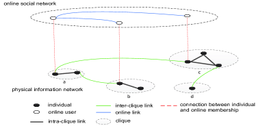
Figure 1: System model $\mathbb{H}$

II-A Topology Structure in System Model

In what follows, we specify the topology structure in the system model $\mathbb{H}$ in Fig. 1.

Cliques in the physical information network. The physical information network has $N$ nodes and the nodes set is denoted by $\mathcal{N}=\{1,2,...,N\}$. These nodes are gathered into many cliques with different sizes. We expect the clique size follows the distribution $\{\mu_{n}^{w},n=1,2,...,D\}$, $n=1,2,...D$, where $D$ is the largest possible size. Therefore, an arbitrary clique could contain $n$ nodes with probability $\mu_{n}^{w}$. We generate these cliques as follows: at step $t=1$, we randomly choose $n$ nodes from the collection $\mathcal{N}$ and create a clique with the selected $n$ nodes, where $n$ is a random number following the distribution $\{\mu_{n}^{w},n=1,2,...,D\}$. We also denote the collection of the remaining nodes in $\mathcal{N}$ by $\mathcal{N}_{1}$. At each step $t$, we repeat the above procedure to create a new clique from the collection $\mathcal{N}_{t-1}$, and assume that we can finally generate $N_{c}$ cliques in $\mathbb{W}$ . Generally speaking, the existence of large size cliques indicates that many individuals are close to each other. In other words, the clique size distribution $\{\mu_{n}^{w}\}$ offers an abstract characterization of personal distances in $\mathbb{W}$ from a macroscopic perspective.

Type-$0$ (intra-clique) links in $\mathbb{W}$. Since the nodes within the same cliques could interact to each other frequently, we assume these nodes are fully connected by type-$0$ links.

Type-$1$ (inter-clique) links in $\mathbb{W}$. We assume that a face-to-face interaction is still possible between cliques, e.g., a person may talk to a remote friend by walking across a long distance. Suppose each node can randomly connect to $k^{w}$ nodes from other cliques through type-$1$ links where $k^{w}$ is a random variable drawn independently from the distribution $\{{p_{k}^{w},k=0,1,...}\}$.

Online users and type-$2$ (online) links. The nodes in the online network $\mathbb{F}$ represent the online users. As in [5], we assume each online user randomly connects to $k^{f}$ online neighbors in $\mathbb{F}$, where $k^{f}$ is a random variable whose distribution is drawn independently from $\{p_{k}^{f},k=0,1,...\}$. We denote such online connection as type-$2$ link. Furthermore, we draw a virtual type-$3$ link from an online user in $\mathbb{F}$ to the actual person it corresponds to in the physical information network $\mathbb{W}$; this indicates that the two nodes actually correspond to the same individual.

Online users associated with a clique. To avoid confusions, we say “size-$n$ clique with $m$ online members” when referring to the case that a clique contains $n$ individuals and only $m$ of them participate in the online social network $\mathbb{F}$. With this insight, we can also differentiate among the collection of size-$n$ cliques according to their affiliated online users. Specifically, for the collection of size-$n$ cliques with $m$ online members, $m\leq n\leq D$, we assume their fraction size in the whole collection of cliques is $\mu_{nm}$. It is easy to see that

$${\mu_{nm}}=\mu_{n}^{w}\left({\begin{array}[]{*{20}{c}}n\\ m\end{array}}\right){\alpha^{m}}{\left({1-\alpha}\right)^{n-m}}~{}~{}\textrm{and}~{}~{}{\mu_{n}^{w}}=\sum\limits_{m=1}^{n}{\mu_{nm}}.$$ (1)

Furthermore, for the collection of cliques with $m$ online users, their fraction size can be given by

$${\mu_{m}^{f}}=\sum\limits_{n=m}^{D}{\mu_{nm}}.$$ (2)

II-B Information Transmissibility

The message can propagate at different speeds along different types of social connections in $\mathbb{H}$. Due to timeliness requirement, the real-time information is easier to pass over a link that offers fast propagation speed. Therefore, we assign each link with a transmissibility as in [5, 9], i.e., the probability that the message can successfully pass through.

From practical scenarios, we set the transmissibility along type-$0$ link as $T_{c}=1$ since the message spreads quickly within a clique. We also define the transmissibilities along type-$1$ and type-$2$ links as $T_{w}$ and $T_{f}$, respectively. Throughout this paper, we say a link is occupied if the message can successfully pass through that link. Hence, in $\mathbb{H}$ each type-$1$ link is occupied independently with probability $T_{w}$, whereas each type-$2$ link is occupied independently with probability $T_{f}$.

II-C Information Cascade

We give a brief description of the information diffusion process in the following. Suppose that the message starts to spread from an arbitrary node $i$ in a clique of $\mathbb{W}$. Then, the other nodes in this clique will quickly receive that message through type-$0$ links. The message can also propagate to other cliques through occupied type-$1$ and type-$2$ links. This in turn may trigger further message propagation and may eventually lead to an information epidemic; i.e., a non-zero fraction of individuals may receive the information in the limit $N\to\infty$.

Clearly, an arbitrary individual can spread the information to nodes that are reachable from itself via the occupied edges of $\mathbb{H}$. Hence, the size of an information outbreak (i.e., the number of individuals that are informed) is closely related to the size of the connected components of $\mathbb{{H}}$, which contains only the occupied type-$1$ and type-$2$ links [5, 9, 8] of $\mathbb{H}$. Thus, the information diffusion process considered here is equivalent to a heterogeneous bond-percolation process over the network $\mathbb{H}$; the corresponding bond percolation is heterogeneous since the occupation probabilities are different for type-$1$ and type-$2$ links. In this paper, we will exploit this relation and find the condition and the size of information epidemics by studying the phase transition properties of $\mathbb{{H}}$. A key observation is that the system $\mathbb{{H}}$ exhibits a phase transition behavior at a critical threshold. Specifically, a giant connected component $G_{H}$ that covers a non-trivial fraction of nodes in $\mathbb{{H}}$ is likely to appear above the critical threshold meaning that information epidemics are possible. Below that critical threshold, all components are small indicating that the fraction of influenced individuals tends to zero in the large system size limit.

It is easy to see that the influenced individuals and cliques correspond to the nodes and cliques in $\mathbb{W}$ that are contained inside $G_{H}$. Hence, we introduce two parameters to evaluate the scale of information diffusion:

• $S_{c}$: The fractional size of influenced cliques in $\mathbb{W}$. Namely, $S_{c}$ corresponds to the ratio of the number of cliques in $G_{H}$ to the total number of cliques in $\mathbb{W}$.

• $S_{n}$: The fractional size of influenced individuals in $\mathbb{W}$. Namely, $S_{n}$ corresponds to the ratio of the number of nodes that belong to the cliques in $G_{H}$ to the total number of nodes in $\mathbb{W}$.

With this insight, we can explore the information diffusion process by characterizing the phase transition behavior of the giant component $G_{H}$.

III Equivalent graph: a clique level approach

In this study, we are particularly interested in the following two questions:

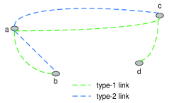
Figure 2: Equivalent graph $\mathbb{E}$. Nodes {a,b,c,d} in this graph corresponds to the cliques {a,b,c,d} of the system $\mathbb{H}$ in Fig. 1. We assign type-$1$ and type-$2$ links in $\mathbb{E}$ according to the same type of links connecting cliques in Fig. 1.

• What is the critical threshold of the system $\mathbb{H}$? In other words, under what condition, the information reaches a non-trival fraction of the network rather than dying out quickly?

• What is the expected size of an information epidemic? In other words, to what fraction of nodes and cliques does the information reach? Or, equivalently, what are the sizes $S_{c}$ and $S_{n}$?

These two questions can be answered by quantifying the phase transition behaviors of the random graph $\mathbb{H}$. Due to the clique structure in our system model, the techniques employed in existing works [5, 8, 9] cannot be directly applied here. To tackle this challenge, we develop an equivalent random graph $\mathbb{E}$ that exhibits the same phase transition behavior as the original model $\mathbb{H}$. Then, we characterize the phase transition behaviors in the graph $\mathbb{E}$ by capitalizing on the recent results in inhomogeneous random graph [10, 11].

We first construct an equivalent graph $\mathbb{E}$ based on the topology structure of $\mathbb{H}$. Since the nodes within the same clique can immediately share the message, we treat each clique including affiliated online users as a single virtual node in $\mathbb{E}$. Furthermore, we assign type-$1$ and type-$2$ links between two virtual nodes according to the original connections in $\mathbb{H}$. To get a more concrete sense, we depict the equivalent graph in Fig. 2 that corresponds to the original model in Fig. 1. It is easy to see that the (type-$1$ and type-$2$) link degree of a virtual node equals the total number of (type-$1$ and type-$2$) links that are incident on the nodes within the corresponding clique. The equivalent graph $\mathbb{E}$ is expected to exhibit the same phase transition behavior as the original model $\mathbb{H}$ since both graphs have the similar connectivity structure. In particular, the fractional size of the giant component $G_{E}$ in the equivalent graph $\mathbb{E}$ (the ratio of the number of nodes in $G_{E}$ to the number of nodes in $\mathbb{E}$) is equal to the aforementioned quantity $S_{c}$. Thus, with a slight abuse of notation, we use $S_{c}$ to denote the fractional size of $G_{E}$.

The degree of an arbitrary node in $\mathbb{E}$ can be represented by a two-dimensional vector $\boldsymbol{d}=[d^{w}\>\>d^{f}]$ where $d^{w}$ and $d^{f}$ correspond to the numbers of type-$1$ and type-$2$ links incident on that node, respectively. For a node in $\mathbb{E}$ that corresponds to a size-$n$ clique in $\mathbb{W}$, we use $K_{n}^{w}$ to denote its type-$1$ link degree, where $K_{n}^{w}$ is a random variable following the distribution $\{P_{nk}^{w},k=0,1,2,...\}$. Similarly, for a node in $\mathbb{E}$ that corresponds to a clique with $m$ online users, we use $K_{m}^{f}$ to denote its type-$2$ link degree where $K_{m}^{f}$ follows the distribution $\{P_{mk}^{f},k=0,1,2,...\}$. It is clear to see that an arbitrary node in $\mathbb{E}$ has link degree $[i\>\>j]$ with probability

$$p(i,j)=\sum\limits_{n=1}^{D}{\sum\limits_{m=0}^{n}{{\mu_{nm}}P_{ni}^{w}P_{mj}^{f}}}~{}~{}~{}i,j\in N.$$ (3)

Let ${\rm{E}}[{d_{w}}]$ and ${\rm{E}}[{d_{f}}]$ be the mean numbers of type-$1$ and type-$2$ links for a node in $\mathbb{E}$, i.e., ${\rm{E}}[{d_{w}}]=\sum\nolimits_{i=0}^{\infty}{\sum\nolimits_{j=0}^{\infty}{p(i,j)i}}$ and ${\rm{E}}[{d_{f}}]=\sum\nolimits_{i=0}^{\infty}{\sum\nolimits_{j=0}^{\infty}{p(i,j)j}}$. We also define ${\rm{E}}[{d_{w}}{d_{f}}]=\sum\nolimits_{i=0}^{\infty}{\sum\nolimits_{j=0}^{\infty}{p(i,j)ij}}$. Furthermore, let ${\rm{E}}[{({d_{w}})^{2}}]$ and ${\rm{E}}[{({d_{f}})^{2}}]$ denote the second moments of the number of type-$1$ and type-$2$ links for a node in $\mathbb{E}$, respectively; i.e., ${\rm{E}}[{({d_{w}})^{2}}]=\sum\nolimits_{i=0}^{\infty}{\sum\nolimits_{j=0}^{\infty}{p(i,j){i^{2}}}}$ and ${\rm{E}}[{({d_{f}})^{2}}]=\sum\nolimits_{i=0}^{\infty}{\sum\nolimits_{j=0}^{\infty}{p(i,j){j^{2}}}}$.

IV Analytical solutions

In this section, we analyze information diffusion process by characterizing the phase transition behaviors in the equivalent random graph $\mathbb{E}$. We present our analytical results in the following two steps. We first quantify the conditions for the emergence of a giant component as well as the fractional sizes $S_{c}$ and $S_{n}$ for the special case $T_{w}=1$ and $T_{f}=1$. We next show that these results can be easily extended to a more general case with $0\leq T_{w}\leq 1$ and $0\leq T_{f}\leq 1$.

IV-A Special Case: $T_{w}=T_{f}=1$

We characterize the phase transition behavior of the giant component in $\mathbb{E}$ by capitalizing the theory of inhomogeneous random graphs [10, 11, 12]. Specifically, we define ${a_{11}}={\rm{E[(}}{d_{w}}{{\rm{)}}^{2}}{\rm{]/E[}}{d_{w}}{\rm{]}}-1$, ${a_{12}}={\rm{E[}}{d_{w}}{{\rm{d}}_{f}}{\rm{]/E[}}{d_{w}}{\rm{]}}$, ${a_{21}}={\rm{E[}}{d_{w}}{{\rm{d}}_{f}}{\rm{]/E[}}{d_{f}}{\rm{]}}$ and ${a_{22}}={\rm{E[(}}{d_{f}}{{\rm{)}}^{2}}{\rm{]/E[}}{d_{f}}{\rm{]}}-1$. Along the same line in [5, 10, 12], we have the following result.

Lemma 4.1

Let

$$\sigma=\frac{1}{2}\left({{a_{11}}+{a_{22}}+\sqrt{{{({a_{11}}-{a_{22}})}^{2}}+4{a_{12}}{a_{21}}}}\right)$$ (4)

if $\sigma>1$, with high probability (whp) there exists a giant component in $\mathbb{E}$, i.e., a non-trival fraction of nodes in $\mathbb{E}$ are connected; otherwise, a giant component does no exist in $\mathbb{E}$ whp.

The proof of Lemma 4.1 is relegated to Appendix A. As we discussed in Section II-C, the existence of a giant component in $\mathbb{E}$ indicates that the information can reach a non-trival fraction of cliques in $\mathbb{H}$ rather than dying out quickly.

Next, let $h_{1}$ and $h_{2}$ in $(0,1]$ be given by the smallest solution to the following recursive equations:

$${h_{1}}=\frac{1}{{{{\rm{E}}[{d_{w}}]}}}\sum\limits_{n=1}^{D}{\sum\limits_{m=0}^{n}{{\mu_{nm}}{\rm{E}}[K_{n}^{w}h_{1}^{K_{n}^{w}-1}]{\rm{E}}[h_{2}^{K_{m}^{f}}]}},$$ (5)

$${h_{2}}=\frac{1}{{{\rm{E}}[{d_{f}}]}}\sum\limits_{n=1}^{D}{\sum\limits_{m=0}^{n}{{\mu_{nm}}{\rm{E}}[h_{1}^{K_{n}^{w}}]{\rm{E}}[K_{m}^{f}h_{2}^{K_{m}^{f}-1}]}}.$$ (6)

We have the following results on the size and probability of an information epidemic.

Lemma 4.2

The fractional size of the giant component in $\mathbb{E}$ (equivalently, the fractional size of influenced cliques in $\mathbb{W}$) is given by

$${S_{c}}=\sum\limits_{n=1}^{D}{\sum\limits_{m=0}^{n}{{\mu_{nm}}\left({1-{\rm{E}}[h_{1}^{K_{n}^{w}}]{\rm{E}}[h_{2}^{K_{m}^{f}}]}\right)}}.$$ (7)

The fractional size of influenced nodes in $\mathbb{W}$ is given by

$${S_{n}}=\frac{1}{C}\sum\limits_{n=1}^{D}{\sum\limits_{m=0}^{n}{n{\mu_{nm}}\left({1-{\rm{E}}[h_{1}^{K_{n}^{w}}]{\rm{E}}[h_{2}^{K_{m}^{f}}]}\right)}},$$ (8)

with the normalization term $C=\sum\limits_{n=1}^{D}{n{\mu_{n}}}$.

The proof of Lemma 4.2 is relegated to Appendix A. For any given set of parameters, Lemma 4.2 reveals the fraction of individuals and cliques that are likely to receive an information that is started from an arbitrary individual. Namely, an information started from an arbitrary individual gives rise to an information epidemic with probability $S_{n}$ (attributed to the possibility that the arbitrary node belongs to the giant component $G_{H}$), and reaches a fraction $S_{n}$ of nodes in the network. Similar conclusions can be drawn in terms of $S_{c}$ for the fraction of cliques that receive the information.

Note that the condition (4) in Lemma 4.1 depends on the first/second moments of $d_{w}$ and $d_{f}$, which boils down to the linear combinations of the first/second moments of $k^{w}$ and $k^{f}$ in the following manner:

$${\rm{E}}[{d_{w}}]=\sum\limits_{n=1}^{D}{\mu_{n}^{w}n{\rm{E}}[k^{w}]}~{}~{}~{}~{}{\rm{E}}[{d_{f}}]=\sum\limits_{m=1}^{D}{\mu_{m}^{f}m{\rm{E}}[k^{f}]},$$ (9)

$${\rm{E}}[{d_{w}}{d_{f}}]=\sum\limits_{n=1}^{D}{\sum\limits_{m=1}^{n}{{\mu_{nm}}nm{\rm{E}}[k^{w}]{\rm{E}}[k^{f}]}},$$ (10)

$${\rm{E}}[{({d_{w}})^{2}}]=\sum\limits_{n=1}^{D}{\mu_{n}^{w}\left({n{\rm{E}}[{{(k^{w})}^{2}}]+({n^{2}}-n){{\left({{\rm{E}}[k^{w}]}\right)}^{2}}}\right)},$$ (11)

$${\rm{E}}[{({d_{f}})^{2}}]=\sum\limits_{m=1}^{D}{\mu_{m}^{f}\left({m{\rm{E}}[{{(k^{f})}^{2}}]+({m^{2}}-m){{\left({{\rm{E}}[k^{f}]}\right)}^{2}}}\right)}.$$ (12)

According to Lemma 4.2, $S_{c}$ and $S_{n}$ are determined by ${\rm{E}}[h_{1}^{K_{n}^{w}}]$, ${\rm{E}}[K_{n}^{w}h_{1}^{K_{n}^{w}-1}]$, ${\rm{E}}[h_{2}^{K_{m}^{f}}]$ and ${\rm{E}}[K_{m}^{f}h_{2}^{K_{m}^{f}-1}]$ in (5)-(8), i.e., the integrals with respect to the distributions of $K_{n}^{w}$ and $K_{m}^{f}$ for different $n$ and $m$. The calculations can be simplified by utilizing the following transformations:

$${\rm{E}}[h_{1}^{K_{n}^{w}}]=({{\rm{E}}[h_{1}^{{k^{w}}}]})^{n}~{}~{}~{}{\rm{E}}[h_{2}^{K_{m}^{f}}]=({{\rm{E}}[h_{2}^{{k^{f}}}]})^{m},$$ (13)

$${\rm{E}}[K_{n}^{w}h_{1}^{K_{n}^{w}-1}]=n{\left({{\rm{E}}[h_{1}^{{k^{w}}}]}\right)^{n-1}}{\rm{E}}[{k^{w}}h_{1}^{{k^{w}}-1}],$$ (14)

$${\rm{E}}[K_{m}^{f}h_{2}^{K_{m}^{f}-1}]=m{\left({{\rm{E}}[h_{2}^{{k^{f}}}]}\right)^{m-1}}{\rm{E}}[{k^{f}}h_{2}^{{k^{f}}-1}].$$ (15)

With the help of (13)-(15), we only need to calculate the integrals with respect to the distributions of $k^{w}$ and $k^{f}$. In this way, we can find $h_{1}$ and $h_{2}$ by numerically solving the recursive equations (5)-(6) and compute $S_{c}$ and $S_{n}$ from (7)-(8), respectively. The detailed derivations of (9)-(15) are omitted (see details in Appendix B).

IV-B General Case: $0\leq T_{w}\leq 1$ and $0\leq T_{f}\leq 1$

We next generalize Lemma 4.1 and Lemma 4.2 to the case $0\leq T_{w}\leq 1$ and $0\leq T_{f}\leq 1$. To this end, we maintain the occupied links in the equivalent graph $\mathbb{E}$ by deleting each type-$1$ and type-$2$ edge with probability $1-T_{w}$ and $1-T_{f}$, respectively. Let ${\tilde{k}^{w}}$ and ${\tilde{k}^{f}}$ be the occupied link degrees (instead of $k^{w}$ and $k^{f}$) with the distributions $\{\tilde{p}_{k}^{w},k=0,1,...\}$ and $\{\tilde{p}_{k}^{f},k=0,1,...\}$. According to [9], the generating functions corresponding to ${\tilde{k}^{w}}$ and ${\tilde{k}^{f}}$ can be given by

$$\tilde{g}(x)=g\left({1+{T_{w}}(x-1)}\right)~{}~{}\tilde{q}(x)=q\left({1+{T_{f}}(x-1)}\right).$$ (16)

From (9)-(15), we observe that the critical threshold and the giant component size are determined by the distributions of $k^{w}$ and $k^{f}$. Therefore, Lemma 4.1 and Lemma 4.2 still hold if we replace the terms associated with $k^{w}$ and $k^{f}$ in (9)-(15) by those associated with ${\tilde{k}^{w}}$ and ${\tilde{k}^{f}}$, respectively. To this end, by using the generating functions (16), we find

$${\rm{E}}[{{\tilde{k}}^{w}}] = {T_{w}}{\rm{E}}[{k^{w}}],$$

$${\rm{E}}[{({{\tilde{k}}^{w}})^{2}}] = T_{w}^{2}\left({{\rm{E}}[{{({k^{w}})}^{2}}]-{\rm{E}}[{k^{w}}]}\right)+{T_{w}}{\rm{E}}[{k^{w}}].$$

In the same manner, we can compute ${\rm{E}}[{{\tilde{k}}^{f}}]$ and ${\rm{E}}[{({{\tilde{k}}^{f}})^{2}}]$. The critical threshold (in the general case) can now be computed by replacing ${\rm{E}}[{{k}^{w}}]$, ${\rm{E}}[{{k}^{f}}]$, ${\rm{E}}[{({{k}^{w}})^{2}}]$, ${\rm{E}}[{({{k}^{f}})^{2}}]$ with ${\rm{E}}[{{\tilde{k}}^{w}}]$, ${\rm{E}}[{{\tilde{k}}^{f}}]$, ${\rm{E}}[{({{\tilde{k}}^{w}})^{2}}]$, ${\rm{E}}[{({{\tilde{k}}^{f}})^{2}}]$, respectively, in (9)-(12).

In order to compute the giant component size, we only need to replace the corresponding terms in (13)-(15) with ${\rm{E}}[h_{1}^{\tilde{k}^{w}}]$, ${\rm{E}}[h_{2}^{\tilde{k}^{f}}]$, ${\rm{E}}[{{\tilde{k}}^{w}}h_{1}^{{{\tilde{k}}^{w}}-1}]$ and ${\rm{E}}[{{\tilde{k}}^{f}}h_{2}^{{{\tilde{k}}^{f}}-1}]$. By using (16), we have

$${\rm{E}}[h_{1}^{\tilde{k}^{w}}]=\tilde{g}({h_{1}})={\rm{E}}[{(1+{T_{w}}({h_{1}}-1))^{{k^{w}}}}],$$

$${\rm{E}}[{{\tilde{k}}^{w}}h_{1}^{{{\tilde{k}}^{w}}-1}]={\left[{\tilde{g}({h_{1}})}\right]^{\prime}}={T_{w}}{\rm{E}}[{k_{w}}{(1+{T_{w}}({h_{1}}-1))^{{k^{w}}-1}}].$$

Similar relations can be obtained for ${\rm{E}}[h_{1}^{\tilde{k}^{f}}]$ and ${\rm{E}}[{{\tilde{k}}^{f}}h_{1}^{{{\tilde{k}}^{f}}-1}]$. The size of the giant component (in the general case) can now be computed by reporting the updated (13)-(15) into (5)-(8).

V Numerical results and simulations

In this section, we numerically study the diffusion of real-time information by utilizing the analytical results derived in Section IV. In particular, we are interested in how the clique structure can impact the scale of information epidemic. To get a more concrete sense, we compare four system scenarios, each with different clique size distribution as illustrated in Table I.

For the sake of fair comparison, the total number of nodes in $\mathbb{W}$ is fixed at $12000$ in each scenario. From Table I, we can see that the average clique size increases from scenario $1$ to scenario $4$, indicating that individuals are getting closer to each other. We assume that the type-$1$ link degree for each node in $\mathbb{W}$ follows a poisson distribution, i.e., $p_{k}^{w}=\frac{{{\lambda^{k}}}}{{k!}}\cdot{e^{-\lambda}}$, $k=0,1,2,...$, where $\lambda$ is the average type-$1$ link degree. Meanwhile, the type-$2$ link degree for each online user in $\mathbb{F}$ follows a power-law distribution with exponential cutoff, i.e., $p_{0}^{f}=0$ and

$$p_{k}^{f}=\frac{1}{C}{k^{-\gamma}}{e^{-\frac{k}{\Gamma}}},\;\;k=1,2,\ldots,$$ (17)

with the normalization factor $C=\sum\limits_{k=1}^{\infty}{{k^{-\gamma}}{e^{-\frac{k}{\Gamma}}}}$.

TABLE I: The clique size distribution in four scenarios

scenario	size-$1$	size-$2$	size-$3$	average clique size
$1$	$100\%$	$0$	$0$	$1$
$2$	$66.7\%$	$33.3\%$	$0$	$1.333$
$3$	$33.3\%$	$66.7\%$	$0$	$1.666$
$4$	$33.3\%$	$33.3\%$	$33.3\%$	$2$

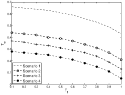
Figure 3: The minimum $T_{w}$ required for the existence of a giant component in $\mathbb{E}$ versus $T_{f}$ in four scenarios. We let $\lambda=1.5$, $\alpha=0.1$, $\gamma=3$ and $\Gamma=10$. Each curve corresponds to the boundary of the phase transition in one scenario. A giant component is very likely to emerge above the boundary.

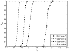
Figure 4: The empirical probability $p_{inf}$ for the existence of giant component is plotted. The simulation results are obtained with $N=12000$ by averaging $200$ experiments. We let $T_{f}=0.4$ and other parameters follow the same setup as in Figure 3. From scenario $1$ to scenario $4$, the values of $p_{inf}$ exhibit a sharp increase at $T_{w}=0.64$, $T_{w}=0.4$, $T_{w}=0.35$ and $T_{w}=0.26$, respectively. Such sharp increase of $p_{inf}$ corresponds to the phase transition. These values are in good agreement with the minimum required $T_{w}$ from the corresponding curves in Figure 3. We assume that a giant component exists if more than $5\%$ of the cliques are connected.

We first compare these scenarios in term of the required conditions for the existence of a giant component; in other words, in terms of the minimum conditions for an information epidemic to take place. We let $\lambda=1.5$, $\alpha=0.1$, $\gamma=3$ and $\Gamma=10$. By computing the system’s critical threshold, we depict in Figure 3 the minimum required value of $T_{w}$ to have a giant component in $\mathbb{E}$ versus $T_{f}$. Each scenario corresponds to a curve in the figure that stands for the boundary of a phase transition; above the boundary a giant component is very likely to emerge. By the definition of transmissibility, a lower required $T_{w}$ indicates that the system is more likely to give rise to a giant component (and thus, to an information epidemic). From scenario $1$ to scenario $4$, this figure clearly shows that larger clique sizes lead to smaller values for the minimum $T_{w}$ required for an information epidemic, meaning that information epidemics are more likely to take place for larger clique sizes. The analytical results of Figure 3 are also verified by simulations. For a fixed $T_{f}$, the probability of the existence of giant component $p_{inf}$ is expected to have a sharp increase as $T_{w}$ approaches to the corresponding minimum required value in Figure 3. Indeed, we observe in Figure 4 that when $T_{f}=0.4$, for each scenario, such sharp transition occur at $T_{w}$ close to the corresponding minimum required value obtained in Figure 3. Such sharp increase of $p_{inf}$ corresponds to the phase transition, i.e., the giant component could exist with high probability above the critical threshold. Therefore, the minimum required $T_{w}$ values obtained via simulations are in good agreement with our analysis.

We next compare these scenarios in terms of the fractional sizes of influenced cliques and influenced individuals. For each scenario, we plot the fractional size of the giant component in $\mathbb{E}$ versus $T_{f}$ in Figure 5, which indicates the fraction of cliques that will receive the information. We set $T_{w}=0.3$, $\lambda=2$, $\alpha=0.3$, $\gamma=3$ and $\Gamma=10$. In this Figure, the curves stand for analytical results obtained by (7), while the marked points stand for the simulation results obtained by averaging $200$ experiments for each set of parameter. It is easy to check that the analytical results are in good agreement with the simulations. Obviously, the fractional size of influenced cliques in scenario $4$ (with average clique size $2$) is much larger than that in scenario $1$ (with average clique size $1$), which indicates that large cliques in the social network could greatly facilitate the message propagation.

We finally compare the fractional size of influenced individuals in Figure 6. In this figure, the curves stand for the fractional size of influenced nodes obtained via (8), whereas the marked points stand for the simulation results. Similar to Figure 5, the information is much easier to propagate in a social network when larger size cliques exist. For instance, when $T_{f}=1$, the fractional size of individuals that receive the message grows sharply from $14\%$ (scenario $1$ with average clique size $1$) to $80\%$ (scenario $4$ with average clique size $2$). In conclusion, the above results agree with a natural conjecture that the messages are more influential (i.e., more likely to reach a large portion of the population) when people are close to each other.

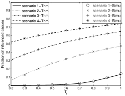
Figure 5: Fraction size of influenced cliques in $\mathbb{W}$ versus $T_{f}$. We set $T_{w}=0.3$, $\lambda=2$, $\alpha=0.3$, $\gamma=3$ and $\Gamma=10$. The curves stand for analytical results obtained by (7), while the marked points stand for the simulation results with $N=12000$ by averaging $200$ experiments for each set of parameter. The analytical results are in good agreement with the simulations.

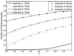
Figure 6: Fraction size of influenced nodes in $\mathbb{W}$ versus $T_{f}$. All the parameters follow the same setup as in Figure 5. The curves stand for analytical results obtained by (8) and the marked points stand for the simulation results with $N=12000$. The analytical results are in good agreement with the simulations. For comparison, we also plot the fraction size of influenced cliques in scenario $1$ where the each clique has only one node.

VI conclusion

In this study, we explore the diffusion of real-time information in social networks. We develop an overlaying social-physical network that consists of an online social network and a physical information network with clique structure. We theoretically quantify the condition and the size of information epidemics. To the best of our knowledge, this paper is the first work on the diffusion of real-time information with consideration on the clique structure in social networks. We believe that our findings will offer initial steps towards understanding the diffusion behaviors of real-time information.

VII Appendix

VII-A Proofs of Lemma 4.1 and Lemma 4.2

In [11, 12] Söderberg studied the phase transition behaviors of inhomogeneous random graphs where nodes are connected by different types of edges. Such graphs are also called “colored degree-driven random graphs” in the sense that different types of edges correspond to different colors. In a graph with $r$-types of edges, the edge degree of an arbitrary node can be represented by a $r$-dimension vector $\boldsymbol{d}=[d^{1}\>\>\cdots\>\>d^{r}]$, where $d^{j}$ stands for the number of type-$j$ edges incident on that node. In our study, the equivalent graph $\mathbb{E}$ has two types of edges and the degree distribution of an arbitrary node is denoted by $p(i,j)={\rm{P[}}{d_{w}}=i,{d_{f}}=j{\rm{]}}$. Also, the generating function of degree distribution $\{p(i,j)\}$ can be defined by $H({x_{1}},{x_{2}})=\sum\nolimits_{i}{\sum\nolimits_{j}{p(i,j)x_{1}^{i}x_{2}^{j}}}$. Clearly, the multivariable combinatorial moments can be achieved by partial differentiation at $x_{1}=1$ and $x_{2}=1$, i.e.,

$${\rm{E[}}{d_{w}}{\rm{]}} = {\partial_{1}}H({x_{1}},{x_{2}}){|_{{x_{1}}={x_{2}}=1}},$$

$${\rm{E[}}{d_{f}}{\rm{]}} = {\partial_{2}}H({x_{1}},{x_{2}}){|_{{x_{1}}={x_{2}}=1}},$$

$${\rm{E[}}{d_{w}}{d_{f}}{\rm{]}} = {\partial_{1}}{\partial_{2}}H({x_{1}},{x_{2}}){|_{{x_{1}}={x_{2}}=1}},$$

$${\rm{E[(}}{d_{w}}{{\rm{)}}^{2}}{\rm{]}} = \partial_{1}^{2}H({x_{1}},{x_{2}}){|_{{x_{1}}={x_{2}}=1}},$$

$${\rm{E[(}}{d_{f}}{{\rm{)}}^{2}}{\rm{]}} = \partial_{2}^{2}H({x_{1}},{x_{2}}){|_{{x_{1}}={x_{2}}=1}}.$$

Let $\{{a_{k}}\}$ denote size distribution of the largest connected component that can be reached from an arbitrary node in $\mathbb{E}$, whose generating function is defined by $g(z)=\sum\nolimits_{k}{{a_{k}}{z^{k}}}$. Furthermore, we define a two-dimension vector $\mathbf{h}(z)=[{h_{1}}(z),{h_{2}}(z)]$, where ${h_{i}}(z)$ stands for the generating function of size distribution of the component connected by type-$i$ edges. According to the existing results in [5, 11, 12], we have that

$$g(z)=z\sum\limits_{i=0}^{\infty}{\sum\limits_{j=0}^{\infty}{p(i,j){h_{1}}{{(z)}^{i}}{h_{2}}{{(z)}^{j}}=zH(\mathbf{h}(z))}},$$ (18)

where $\mathbf{h}(z)$ satisfies the following recursive equations

$${h_{1}}(z) = \frac{z}{{{\rm{E[}}{d_{w}}{\rm{]}}}}{\partial_{1}}H(h(z)),$$ (19)

$${h_{2}}(z) = \frac{z}{{{\rm{E[}}{d_{f}}{\rm{]}}}}{\partial_{2}}H(h(z)).$$ (20)

The emergence of giant component in $\mathbb{E}$ can be checked by examining the stability of the recursive equations (19)-(20) at the point ${h_{1}}={h_{1}}(1)=1$ and ${h_{2}}={h_{2}}(1)=1$. Along the same line as in [11, 12], we define a $2\times 2$ Jacobian matrix $\mathbf{J}$, i.e.,

$$\mathbf{J}=\left[{\begin{array}[]{*{20}{c}}{{a_{11}}}&{{a_{12}}}\\ {{a_{21}}}&{{a_{22}}}\\ \end{array}}\right],$$

where

$${a_{11}} = \frac{1}{{{\rm{E[}}{d_{w}}{\rm{]}}}}\partial_{1}^{2}H(h(z)){|_{{h_{1}}={h_{2}}=1}}={{{\rm{E[(}}{d_{w}}{{\rm{)}}^{2}}{\rm{-}}{d_{w}}{\rm{]}}}\mathord{\left/{\vphantom{{{\rm{E[(}}{d_{w}}{{\rm{)}}^{2}}{\rm{-}}{d_{w}}{\rm{]}}}{{\rm{E[}}{d_{w}}{\rm{]}}}}}\right.\kern-1.2pt}{{\rm{E[}}{d_{w}}{\rm{]}}}},$$

$${a_{12}} = \frac{1}{{{\rm{E[}}{d_{w}}{\rm{]}}}}\partial_{1}\partial_{2}H(h(z)){|_{{h_{1}}={h_{2}}=1}}={{{\rm{E[}}{d_{w}}{d_{f}}{\rm{]}}}\mathord{\left/{\vphantom{{{\rm{E[}}{d_{w}}{d_{f}}{\rm{]}}}{{\rm{E[}}{d_{w}}{\rm{]}}}}}\right.\kern-1.2pt}{{\rm{E[}}{d_{w}}{\rm{]}}}},$$

$${a_{21}} = \frac{1}{{{\rm{E[}}{d_{f}}{\rm{]}}}}\partial_{1}\partial_{2}H(h(z)){|_{{h_{1}}={h_{2}}=1}}={{{\rm{E[}}{d_{w}}{d_{f}}{\rm{]}}}\mathord{\left/{\vphantom{{{\rm{E[}}{d_{w}}{d_{f}}{\rm{]}}}{{\rm{E[}}{d_{f}}{\rm{]}}}}}\right.\kern-1.2pt}{{\rm{E[}}{d_{f}}{\rm{]}}}},$$

$${a_{22}} = \frac{1}{{{\rm{E[}}{d_{f}}{\rm{]}}}}\partial_{2}^{2}H(h(z)){|_{{h_{1}}={h_{2}}=1}}={{{\rm{E[(}}{d_{f}}{{\rm{)}}^{2}}{\rm{-}}{d_{f}}{\rm{]}}}\mathord{\left/{\vphantom{{{\rm{E[(}}{d_{f}}{{\rm{)}}^{2}}{\rm{-}}{d_{f}}{\rm{]}}}{{\rm{E[}}{d_{f}}{\rm{]}}}}}\right.\kern-1.2pt}{{\rm{E[}}{d_{f}}{\rm{]}}}}.$$

The spectral radius of $\mathbf{J}$ is given by

$$\sigma=\frac{1}{2}\left({{a_{11}}+{a_{22}}+\sqrt{{{({a_{11}}-{a_{22}})}^{2}}+4{a_{12}}{a_{21}}}}\right).$$

By [5, 10, 12], if $\sigma>1$, with high probability there exist a giant component in the graph $\mathbb{E}$;otherwise, a giant component is very less likely to exist in $\mathbb{E}$. Therefore, the condition (4) in Lemma 4.1 is achieved. Furthermore, the fraction size $S_{c}$ equals $1-g(1)$ [5]. By (18), we have that

$${S_{c}} = 1-g(1)=\sum\limits_{i=0}^{\infty}{\sum\limits_{j=0}^{\infty}{p(i,j)\left({1-h_{1}^{i}h_{2}^{j}}\right)}}$$

$$= \sum\limits_{n=1}^{D}{\sum\limits_{m=0}^{n}{{\mu_{nm}}{\sum\limits_{i=0}^{\infty}{\sum\limits_{j=0}^{\infty}{P_{ni}^{w}P_{mj}^{f}\left({1-h_{1}^{i}h_{2}^{j}}\right)}}}}}$$

$$= \sum\limits_{n=1}^{D}{\sum\limits_{m=0}^{n}{{\mu_{nm}}\left({1-\sum\limits_{i=0}^{\infty}{\sum\limits_{j=0}^{\infty}{P_{ni}^{w}P_{mj}^{f}h_{1}^{i}h_{2}^{j}}}}\right)}}$$

$$= \sum\limits_{n=1}^{D}{\sum\limits_{m=0}^{n}{{\mu_{nm}}\left({1-{\rm{E}}[h_{1}^{K_{n}^{w}}]{\rm{E}}[h_{2}^{K_{m}^{f}}]}\right)}}.$$

In view of (19) and (20), we have that

$${h_{1}} = \frac{1}{{{{\rm{E}}[{d_{w}}]}}}\sum\limits_{i=0}^{\infty}{\sum\limits_{j=0}^{\infty}{p(i,j)ih_{1}^{i-1}h_{2}^{j}}}$$

$$= \frac{1}{{{{\rm{E}}[{d_{w}}]}}}\sum\limits_{n=1}^{D}{\sum\limits_{m=0}^{n}{{\mu_{nm}}{\rm{E}}[K_{n}^{w}h_{1}^{K_{n}^{w}-1}]{\rm{E}}[h_{2}^{K_{m}^{f}}]}},$$

$${h_{2}} = \frac{1}{{{{\rm{E}}[{d_{f}}]}}}\sum\limits_{i=0}^{\infty}{\sum\limits_{j=0}^{\infty}{p(i,j)jh_{1}^{i}h_{2}^{j-1}}}$$

$$= \frac{1}{{{\rm{E}}[{d_{f}}]}}\sum\limits_{n=1}^{D}{\sum\limits_{m=0}^{n}{{\mu_{nm}}{\rm{E}}[h_{1}^{K_{n}^{w}}]{\rm{E}}[K_{m}^{f}h_{2}^{K_{m}^{f}-1}]}}.$$

Furthermore, (VII-A) can be rewritten in the following form:

$$S_{c}=\sum\limits_{i=0}^{\infty}{\sum\limits_{j=0}^{\infty}\sum_{n=1}^{D}\sum_{m=0}^{n}\mu_{nm}P_{ni}^{w}P_{mj}^{f}{(1-h_{1}^{i}h_{2}^{j})}}.$$

Clearly, the term in parentheses gives the probability that a node with colored degree $[{d_{w}}=i,{d_{f}}=j]$ belongs to the giant component. In other words, the term in parentheses is the expected number of cliques added to the giant cluster by a degree $[{d_{w}}=i,{d_{f}}=j]$ clique. Hence, summing over all such $i,j$’s we get an expression for the expected size of the giant cluster (in terms of number of cliques).

In order to compute the expected giant component size in terms of the number of nodes, namely to compute $S_{n}$, we can modify the above expression such that the term $n(1-h_{1}^{i}h_{2}^{j})$ gives the expected number of nodes to be included in the giant cluster by a degree $[{d_{w}}=i,{d_{f}}=j]$ clique. In other words, with probability $(1-h_{1}^{i}h_{2}^{j})$ the clique under consideration will belong to the giant component $G_{H}$ and will bring $n$ nodes to the actual giant size $S_{n}$. This yields

$${\bar{S}_{n}} = \sum\limits_{i=0}^{\infty}{\sum\limits_{j=0}^{\infty}{\sum\limits_{n=1}^{D}{\sum\limits_{m=0}^{n}{{\mu_{nm}}}}P_{ni}^{w}P_{mj}^{f}n\left({1-h_{1}^{i}h_{2}^{j}}\right)}}$$

$$= \sum\limits_{n=1}^{D}{\sum\limits_{m=0}^{n}{n{\mu_{nm}}}}\sum\limits_{i=0}^{\infty}{\sum\limits_{j=0}^{\infty}{P_{ni}^{w}P_{mj}^{f}\left({1-h_{1}^{i}h_{2}^{j}}\right)}}$$

$$= \sum\limits_{n=1}^{D}{\sum\limits_{m=0}^{n}{n{\mu_{nm}}\left({1-\sum\limits_{i=0}^{\infty}{\sum\limits_{j=0}^{\infty}{P_{ni}^{w}P_{mj}^{f}h_{1}^{i}h_{2}^{j}}}}\right)}}$$

$$= \sum\limits_{n=1}^{D}{\sum\limits_{m=0}^{n}{n{\mu_{nm}}\left({1-{\rm{E}}[h_{1}^{K_{n}^{w}}]{\rm{E}}[h_{2}^{K_{m}^{f}}]}\right)}}.$$

We next have

$${S_{n}}=\frac{1}{C}{\bar{S}_{n}},~{}~{}~{}C=\sum\limits_{n=1}^{D}{n{\mu_{n}}},$$

where the normalized term $C$ makes $S_{n}=1$ at $h_{1}=h_{2}=0$. Therefore, the conclusions (7) and (8) in Lemma 4.2 have been obtained.

VII-B Detailed Derivations for Equations (9)-(15)

As defined in Section III, $K_{n}^{w}$ is the sum of $n$ independent copies of $k^{w}$ and $K_{m}^{f}$ is the sum of $m$ independent copies of $k^{f}$. It follows that

$${\rm{E}}[K_{n}^{w}]=n{\rm{E}}[k^{w}]~{}~{}~{}~{}{\rm{E}}[K_{m}^{f}]=m{\rm{E}}[k^{f}],$$

$${\rm{E}}[{(K_{n}^{w})^{2}}] = {\mathop{\rm var}}[K_{n}^{w}]+{\left({{\rm{E}}[K_{n}^{w}]}\right)^{2}}$$

$$= n{\rm{E}}[{(k^{w})^{2}}]+({n^{2}}-n){\left({{\rm{E}}[k^{w}]}\right)^{2}},$$

$${\rm{E}}[{(K_{m}^{f})^{2}}] = {\mathop{\rm var}}[K_{m}^{f}]+{\left({{\rm{E}}[K_{m}^{f}]}\right)^{2}}$$

$$= m{\rm{E}}[{(k^{f})^{2}}]+({m^{2}}-m){\left({{\rm{E}}[k^{f}]}\right)^{2}}.$$

In view of this, we can rewrite the first/second moments of $d_{w}$ and $d_{f}$ as follows:

$${\rm{E}}[{d_{w}}] = \sum\limits_{i=0}^{\infty}{\sum\limits_{j=0}^{\infty}{p(i,j)i}}$$

$$= \sum\limits_{n=1}^{D}{\sum\limits_{m=0}^{n}{{\mu_{nm}}\left({\sum\limits_{i=0}^{\infty}{\sum\limits_{j=0}^{\infty}{iP_{ni}^{w}P_{mj}^{f}}}}\right)}}$$

$$= \sum\limits_{n=1}^{D}{\sum\limits_{m=0}^{n}{{\mu_{nm}}{\rm{E}}[}K_{n}^{w}}]=\sum\limits_{n=1}^{D}{\mu_{n}^{w}n{\rm{E}}[k^{w}]},$$

$${\rm{E}}[{d_{f}}] = \sum\limits_{i=0}^{\infty}{\sum\limits_{j=0}^{\infty}{p(i,j)j}}$$

$$= \sum\limits_{n=1}^{D}{\sum\limits_{m=0}^{n}{{\mu_{nm}}\left({\sum\limits_{i=0}^{\infty}{\sum\limits_{j=0}^{\infty}{jP_{ni}^{w}P_{mj}^{f}}}}\right)}}$$

$$= \sum\limits_{n=1}^{D}{\sum\limits_{m=0}^{n}{{\mu_{nm}}{\rm{E}}[}K_{m}^{f}}]=\sum\limits_{m=1}^{D}{\mu_{m}^{f}m{\rm{E}}[k^{f}]},$$

$${\rm{E}}[{d_{w}}{d_{f}}] = \sum\limits_{i=0}^{\infty}{\sum\limits_{j=0}^{\infty}{p(i,j)i}}j$$

$$= \sum\limits_{n=1}^{D}{\sum\limits_{m=1}^{n}{{\mu_{nm}}nm{\rm{E}}[k^{w}]{\rm{E}}[k^{f}]}},$$

$${\rm{E}}[{({d_{w}})^{2}}]=\sum\limits_{i=0}^{\infty}{\sum\limits_{j=0}^{\infty}{p(i,j){i^{2}}=\sum\limits_{n=1}^{D}{\mu_{n}^{w}E[{{(K_{n}^{w})}^{2}}]}}}$$

$$=\sum\limits_{n=1}^{D}{\mu_{n}^{w}\left({n{\rm{E}}[{{(k^{w})}^{2}}]+({n^{2}}-n){{\left({{\rm{E}}[k^{w}]}\right)}^{2}}}\right)},$$

$${\rm{E}}[{({d_{f}})^{2}}]=\sum\limits_{i=0}^{\infty}{\sum\limits_{j=0}^{\infty}{p(i,j){j^{2}}=\sum\limits_{m=1}^{D}{\mu_{m}^{f}E[{{(K_{m}^{f})}^{2}}]}}}$$

$$=\sum\limits_{m=1}^{D}{\mu_{m}^{f}\left({m{\rm{E}}[{{(k^{f})}^{2}}]+({m^{2}}-m){{\left({{\rm{E}}[k^{f}]}\right)}^{2}}}\right)}.$$

We next characterize the generating functions of $K_{n}^{w}$ and $K_{m}^{f}$. Specifically, the generating functions of the type-$1$ and type-$2$ link degree distribution for a single node in $\mathbb{H}$ can be defined by $g(x)=\sum\nolimits_{k=1}^{\infty}{p_{k}^{w}{x^{k}}}$ and $q(x)=\sum\nolimits_{k=1}^{\infty}{p_{k}^{f}{x^{k}}}$. Since $K_{n}^{w}$ and $K_{m}^{f}$ are sums of i.i.d. random variables, their generating functions of turn out to be

$${G_{n}}(x)=\sum\limits_{k=0}^{\infty}{P_{nk}^{w}{x^{k}}}={\left[{g(x)}\right]^{n}}~{}~{}~{}~{}~{}1\leq n\leq D,$$ (22)

$${Q_{m}}(x)=\sum\limits_{k=0}^{\infty}{P_{mk}^{f}{x^{k}}}=\left\{{\begin{array}[]{*{20}{c}}{{{\left[{q(x)}\right]}^{m}}}~{}~{}~{}1\leq m\leq D,\\ 0~{}~{}~{}~{}~{}~{}~{}~{}~{}~{}m=0\\ \end{array}}\right.$$ (23)

With (22) and (23), ${\rm{E}}[h_{1}^{K_{n}^{w}}]$, ${\rm{E}}[K_{n}^{w}h_{1}^{K_{n}^{w}-1}]$, ${\rm{E}}[h_{2}^{K_{m}^{f}}]$ and ${\rm{E}}[K_{m}^{f}h_{2}^{K_{m}^{f}-1}]$ can boil down to the expected value with respect to the distribution of $k^{w}$ and $k^{f}$ as follows.

$$\begin{array}[]{l}{\rm{E}}[h_{1}^{K_{n}^{w}}]={G_{n}}({h_{1}})={\left({g({h_{1}})}\right)^{n}}=({{\rm{E}}[h_{1}^{{k^{w}}}]})^{n}\\ {\rm{E}}[h_{2}^{K_{m}^{f}}]=Q_{m}({h_{2}})={\left({q({h_{2}})}\right)^{m}}=({{\rm{E}}[h_{2}^{{k^{f}}}]})^{m}\end{array}$$

$${\rm{E}}[K_{n}^{w}h_{1}^{K_{n}^{w}-1}] = {G_{n}}({h_{1}})^{\prime}=n{\left({g({h_{1}})}\right)^{n-1}}{\left({g({h_{1}})}\right)^{\prime}}$$

$$= n{\left({{\rm{E}}[h_{1}^{{k^{w}}}]}\right)^{n-1}}{\rm{E}}[{k^{w}}h_{1}^{{k^{w}}-1}]$$

$${\rm{E}}[K_{m}^{f}h_{2}^{K_{m}^{f}-1}] = {Q_{m}}({h_{2}})^{\prime}=m{\left({q({h_{2}})}\right)^{m-1}}{\left({q({h_{2}})}\right)^{\prime}}$$

$$= m{\left({{\rm{E}}[h_{2}^{{k^{f}}}]}\right)^{m-1}}{\rm{E}}[{k^{f}}h_{2}^{{k^{f}}-1}].$$

References

• [1] A. Mislove, M. Marcon, K.P. Gummadi, P. Druschel, and B. Bhattacharjee. Measurement and analysis of online social networks. In Proceedings of the 7th ACM SIGCOMM Conference on Internet measurement, 2007.
• [2] J. Leskovec, L.A. Adamic, and B.A. Huberman. The dynamics of viral marketing. ACM Transactions on the Web (TWEB), 1(1):5, 2007.
• [3] L. Isella, J. Stehlé, A. Barrat, C. Cattuto, J.F. Pinton, and W. Van den Broeck. What’s in a crowd? Analysis of face-to-face behavioral networks. Journal of Theoretical Biology, 2010.
• [4] K. Zhao, J. Stehle, G. Bianconi, and A. Barrat. Social network dynamics of face-to-face interactions. Phys. Rev. E, 83(5):056109, 2011.
• [5] O. Yagan, D. Qian, J. Zhang, and D. Cochran. Conjoining speeds up information diffusion in overlaying social-physical networks. Technical report, Available online at arXiv:1112.4002v1[cs.SI],.
• [6] J. Yang and J. Leskovec. Modeling information diffusion in implicit networks. In Proceedings of the 10th IEEE International Conference on Data Mining, 2010.
• [7] J. Stehlé, A. Barrat, and G. Bianconi. Dynamical and bursty interactions in social networks. Phys. Rev. E, 81(3):035101, 2010.
• [8] M. E. J. Newman, S. H. Strogatz, and D. J. Watts. Random graphs with arbitrary degree distributions and their applications. Phys. Rev. E, 64(2), 2001.
• [9] M. E. J. Newman. Spread of epidemic disease on networks. Phys. Rev. E, 66(1), 2002.
• [10] B. Söderberg. General formalism for inhomogeneous random graphs. Phys. Rev. E, 66(066121), 2002.
• [11] B. Söderberg. Random graphs with hidden color. Phys. Rev. E, 68(015102(R)), 2003.
• [12] B. Söderberg. Random graph models with hidden color. Acta Phys. Pol. B, 34:5085–5102, 2003.