HADWIGER’S THEOREM FOR DEFINABLE FUNCTIONS

Abstract.

Hadwiger’s Theorem states that ${\mathbb{E}}_{n}$-invariant convex-continuous valuations of definable sets in ⁿ are linear combinations of intrinsic volumes. We lift this result from sets to data distributions over sets, specifically, to definable -valued functions on ⁿ. This generalizes intrinsic volumes to (dual pairs of) non-linear valuations on functions and provides a dual pair of Hadwiger classification theorems.

1. Introduction

Let ⁿ denote Euclidean $n$-dimensional space. A valuation on a collection $\mathcal{S}$ of subsets of ⁿ is an additive function $v:\mathcal{S}\to\real$:

(1) $$v(A)+v(B)=v(A\cap B)+v(A\cup B)\qquad\text{whenever }A,B,A\cap B,A\cup B\in\mathcal{S}.$$

Valuation $v$ is ${\mathbb{E}}_{n}$-invariant if $v(\varphi A)=v(A)$ for all $A\in\mathcal{S}$ and $\varphi\in{\mathbb{E}}_{n}$, the group of Euclidean (or rigid) motions in ⁿ. A classical theorem of Hadwiger [16] states that the ${\mathbb{E}}_{n}$-invariant continuous valuations on compact convex sets $\mathcal{S}$ in ⁿ (here a valuation is continuous with respect to convergence of sets in the Hausdorff metric) form a finite-dimensional -vector space generated by intrinsic volumes $\mu_{k}$, $k=0,\ldots,n$.

Theorem 1 (Hadwiger).

Any ${\mathbb{E}}_{n}$-invariant continuous valuation $v$ on compact convex subsets of ⁿ is a linear combination of the intrinsic volumes:

(2) $$v=\sum_{k=0}^{n}c_{k}\mu_{k}\,,$$

for some constants $c_{k}\in\real$. If $v$ is homogeneous of degree $k$, then $v=c_{k}\mu_{k}$.

The intrinsic volumes $\mu_{k}$ are characterized uniquely by (1) ${\mathbb{E}}_{n}$ invariance, (2) normalization with respect to a closed unit ball, and (3) homogeneity: $\mu_{k}(\lambda\cdot A)=\lambda^{k}(A)$ for all $A\in\mathcal{S}$ and $\lambda\in{}^{+}$. These measures generalize Euclidean $n$-dimensional volume ($\mu_{n}$) and Euler characteristic ($\mu_{0}$).

This paper extends Hadwiger’s Theorem to similar valuations on functions instead of sets. Section 2 gives background on the definable (o-minimal) setting that lifts Hadwiger’s Theorem to tame, non-convex sets and then to constructible functions; there, we also review the convex-geometric, integral-geometric, and sheaf-theoretic approaches to Hadwiger’s Theorem. In Section 4, we consider definable functions $\mathbf{Def}({}^{n})$ as -valued functions with tame graphs, and correspondingly define dual pairs of (typically) non-linear “integral” operators $\int\cdot{\lfloor d\mu_{k}\rfloor}$ and $\int\cdot{\lceil d\mu_{k}\rceil}$ mapping $\mathbf{Def}({}^{n})\to\real$ as generalizations of intrinsic volumes, so that $\int{\mathbf{1}}_{A}{\lfloor d\mu_{k}\rfloor}=\mu_{k}(A)=\int{\mathbf{1}}_{A}{\lceil d\mu_{k}\rceil}$ for all $A$ definable. These integrals are ${\mathbb{E}}_{n}$-invariant and satisfy generalized homogeneity and additivity conditions reminiscent of intrinsic volumes; they are furthermore compact-continuous with respect to a dual pair of topologies on functions. This culminates in Section 6 in a generalization of Hadwiger’s Theorem for functions:

Theorem 2 (Main).

Any ${\mathbb{E}}_{n}$-invariant definably lower- (resp. upper-) continuous valuation $v:\mathbf{Def}({}^{n})\to\real$ is of the form:

(3) $$v(h)=\sum_{k=0}^{n}\left(\int_{{}^{n}}c_{k}\circ h{\lfloor d\mu_{k}\rfloor}\right)$$

(resp., integrals with respect to ${\lceil d\mu_{k}\rceil}$) for some $c_{k}\in C(\real)$ continuous and monotone, satisfying $c_{k}(0)=0$.

The $k=0$ intrinsic measure ${\lfloor d\mu_{0}\rfloor}$ is a recent generalization ${\lfloor d\chi\rfloor}$ of Euler characteristic [7] shown to have applications to signal processing [14] and Gaussian random fields [8]. The $k=n$ intrinsic measure ${\lfloor d\mu_{n}\rfloor}$ is Lebesgue volume. The measures come in dual pairs ${\lfloor d\mu_{k}\rfloor}$ and ${\lceil d\mu_{k}\rceil}$ as a manifestation of (Verdier-Poincaré) duality. Our results yield the following:

Corollary 3.

Any ${\mathbb{E}}_{n}$-invariant valuation, both upper- and lower-continuous, is a weighted Lebesgue integral.

We conclude the Introduction remarking that over the past few years several very interesting papers by M. Ludwig, A. Tsang and others appeared, that deal with valuations (often tensor- or set-valued) on various functional spaces (such as $L_{p}$ and Sobolev spaces): for a recent report, see [21]. Our approach deviates from this circle of results primarily in the choice of the functional space: definable functions form a distinctly different domain for the valuation. The quite fine topologies we impose on the definable functions yield a rich supply of the valuations continuous in these topologies.

2. Background

2.1. Euler characteristic

Intrinsic volumes are built upon the Euler characteristic. Among the many possible approaches to this topological invariant — combinatorial [17], cohomological [15], sheaf-theoretic [25, 26], we use the language of o-minimal geometry [29]. An o-minimal structure is a sequence ${\mathcal{O}}=(O_{n})_{n}$ of Boolean algebras of subsets of ⁿ which satisfy a few basic axioms (closure under cross products and projections; algebraic basis; and $O_{1}$ consists of finite unions of points and open intervals). Examples of o-minimal structures include the semialgebraic sets, globally subanalytic sets, and (by slight abuse of terminology) semilinear sets; more exotic structures with exponentials also occur [29]. The details of o-minimal geometry can be ignored in this paper, with the following exceptions:

1. Elements of ${\mathcal{O}}$ are called tame or, more properly, definable sets.

2. A mapping between definable sets is definable if and only if its graph is a definable set.

3. The basic equivalence relation on definable sets is definable bijection; these are not necessarily continuous.

4. The Triangulation Theorem [29, Thm 8.1.7, p. 122]: any definable set $Y$ is definably equivalent to a finite disjoint union of open simplices $\{\sigma\}$ of different dimensions.

5. The Hardt Theorem [29]: for $f:X\to Y$ definable, $Y$ has a triangulation into open simplices $\{\sigma\}$ such that $f^{-1}(\sigma)$ is homeomorphic to $U_{\sigma}\times\sigma$ for $U_{\sigma}$ definable, and, on this inverse image, $f$ acts as projection.

For more information, the reader is encouraged to consult [29, 10, 24].

The (o-minimal) Euler characteristic is the valuation $\chi$ that evaluates to $(-1)^{k}$ on an open $k$-simplex. It is well-defined and invariant under definable bijection [29, Sec. 4.2], and, among definable sets of fixed dimension (the dimension of the largest cell in a triangulation), is a complete invariant of definable sets up to definable bijection. Note that the o-minimal Euler characteristic coincides with the homological Euler characteristic (alternating sum of ranks of homology groups) on compact definable sets. For locally compact definable sets, it has a cohomological definition (alternating sum of ranks of compactly-supported sheaf cohomology), yielding invariance with respect to proper homotopy.

2.2. Intrinsic volumes

Intrinsic volumes have a rich history (see, e.g., [5, 9, 17, 27]) and as many formulations as names, including the following:

Slices: One way to define the intrinsic volume $\mu_{k}(A)$ of a definable set $A$ is in terms of the Euler characteristic of all slices of $A$ along affine codimension-$k$ planes:

(4) $$\mu_{k}(A)=\int_{{\mathcal{P}}_{n,n-k}}\chi(A\cap P)\ d\lambda(P),$$

where $\lambda$ is the following measure on ${\mathcal{P}}_{n,n-k}$, the space of affine $(n-k)$-planes in ⁿ. Each affine subspace $P\in{\mathcal{P}}_{n,n-k}$ is a translation of some linear subspace $L\in{\mathcal{G}}_{n,n-k}$, the Grassmannian of $(n-k)$-dimensional subspaces of ⁿ. That is, $P$ is uniquely determined by $L$ and a vector $\mathbf{x}\in L^{\bot}$, such that $P=L+\mathbf{x}$. Thus, we can integrate over ${\mathcal{P}}_{n,n-k}$ by first integrating over $L^{\bot}$ and then over ${\mathcal{G}}_{n,n-k}$. Equation (4) is equivalent to

(5) $$\mu_{k}(A)=\int_{{\mathcal{G}}_{n,n-k}}\int_{{}^{n}/L}\chi(A\cap(L+\mathbf{x}))\ d\mathbf{x}\ d\gamma(L),$$

where $L\in{\mathcal{G}}_{n,n-k}$, the factorspace ${}^{n}/L$ is given the natural Lebesgue measure, and $\gamma$ is the Haar (i.e. $\mathit{SO}(n)$-invariant) measure on the Grassmannian, scaled appropriately.

Projections: Dual to the above definition, one can express $\mu_{k}$ in terms of projections onto $k$-dimensional linear subspaces: for any definable $A\subset{}^{n}$ and $0\leq k\leq n$,

(6) $$\mu_{k}(A)=\int_{{\mathcal{G}}_{n,k}}\int_{L}\chi(\pi_{L}^{-1}(\mathbf{x}))\ d\mathbf{x}\ d\gamma(L)$$

where $L\in{\mathcal{G}}_{n,k}$ and $\pi_{L}^{-1}(\mathbf{x})$ is the fiber over $\mathbf{x}\in L$ of the orthogonal projection map $\pi:A\to L$. For $A$ convex, Equation (6) reduces to

$$\mu_{k}(A)=\int_{{\mathcal{G}}_{n,k}}\mu_{k}(A|L)\ d\gamma(L)$$

where the integrand is the $k$-dimensional (Lebesgue) volume of the projection of $A$ onto a $k$-dimensional subspace $L$ of ⁿ.

2.3. Normal, conormal, and characteristic cycles

Perspectives from geometric measure theory and sheaf theory are also relevant to the definition of intrinsic volumes. In this section, we restrict to the o-minimal structure of globally subanalytic sets and use analytic tools based on geometric measure theory, following Alesker [3, 4], Fu [12], Nicolaescu [23, 24] and many others.

Let $\Omega^{k}_{c}({}^{n})$ be the space of differential $k$-forms on ⁿ with compact support. Let $\Omega_{k}({}^{n})$ be the space of $k$-currents — the topological dual of $\Omega_{c}^{k}({}^{n})$. Given any $k$-current $T\in\Omega_{k}({}^{n})$, the boundary of $T$ is $\partial T\in\Omega_{k-1}({}^{n})$ defined as the adjoint to the exterior derivative $d$. A cycle is a current with null boundary.

It is customary to use the flat topology on currents [11]. The mass of a $k$-current $T$ is

(7) $$\mathbf{M}(T)=\sup\left\{T(\omega):\omega\in\Omega_{c}^{k}({}^{n})\ \text{and}\sup_{x\in{}^{n}}|\omega(x)|\leq 1\right\}$$

($|\omega|$ is the usual norm), which generalizes the volume of a submanifold. The flat norm of a $k$-current $T$ is

(8) $$\left|T\right|_{\flat}=\inf\left\{\mathbf{M}(R)+\mathbf{M}(S):T=R+\partial S,R\in\mathcal{R}_{k}({}^{n}),S\in\mathcal{R}_{k+1}({}^{n})\right\},$$

where $\mathcal{R}_{k}$ is the space of rectifiable $k$-currents. The flat norm quantifies the minimal-mass decomposition of a $k$-current $T$ into a $k$-current $R$ and the boundary of a $(k+1)$-current $S$.

Normal cycle: The normal cycle of a compact definable set $A$ is a definable $(n-1)$-current $\mathbf{N}^{A}$ on the unit sphere cotangent bundle $U^{*}{}^{n}\cong S^{n-1}\times{}^{n}$ that is Legendrian with respect to the canonical 1-form $\alpha$ on $T^{*}{}^{n}$. The normal cycle generalizes the unit normal bundle of an embedded submanifold to compact definable sets. The normal cycle is additive: for $A$ and $B$ compact and definable,

(9) $$\mathbf{N}^{A\cup B}+\mathbf{N}^{A\cap B}=\mathbf{N}^{A}+\mathbf{N}^{B}.$$

The intrinsic volume $\mu_{k}$ is representable as integration of a particular (non-unique) form $\alpha_{k}\in\Omega^{n-1}U^{*}{}^{n}$ against the normal cycle:

(10) $$\mu_{k}(A)=\int_{\mathbf{N}^{A}}\alpha_{k}.$$

Fu [12] gives a formula for the normal cycle in terms of stratified Morse theory; Nicolaescu [24] gives a nice description of the normal cycle from Morse theory.

Conormal cycle: The conormal cycle (also known as the characteristic cycle [18, 20, 26]) of a compact definable set $A$ is a Lagrangian $n$-current $\mathbf{C}^{A}$ on $T^{*}{}^{n}$ that generalizes the cone of the unit normal bundle. Indeed, the conormal cycle is the cone over the normal cycle. An intrinsic description for $A$ a submanifold-with-corners is that the conormal cycle is the union of duals to tangent cones at points of $A$. The conormal cycle is additive: for $A$ and $B$ definable,

(11) $$\mathbf{C}^{A\cup B}+\mathbf{C}^{A\cap B}=\mathbf{C}^{A}+\mathbf{C}^{B}.$$

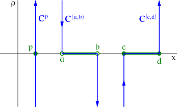
Figure 1. Conormal cycles of the point $p$, the open interval $(a,b)$, and the closed interval $[c,d]$ illustrate the additivity of the conormal cycle.

The intrinsic volume $\mu_{k}$ is representable as integration of a certain (non-unique) form $\omega_{k}\in\Omega^{n}T^{*}{}^{n}$ (supported by a bounded neighborhood of the zero section of the cotangent bundle) against the conormal cycle:

(12) $$\mu_{k}(A)=\int_{\mathbf{C}^{A}}\omega_{k}.$$

As the conormal cycles are cones, one can always rescale the forms $\omega_{k}$ so that they are supported in a given neighborhood of the zero section of the cotangent bundle. We fix the neighborhood once and for all, and will assume henceforth that all $\omega_{k}$ are supported in the unit ball bundle $B_{1}^{*}{}^{n}:=\{|P|\leq 1\}\subset T^{*}{}^{n}$.

The microlocal index theorem [20, 26] gives an interpretation of the conormal cycle in terms of stratified Morse theory.

Continuity: The flat norm on conormal cycles yields a topology on definable subsets on which the intrinsic volumes are continuous. For definable subsets $A$ and $B$, define the flat metric by

(13) $$d_{\flat}(A,B)=\left|(\mathbf{C}^{A}-\mathbf{C}^{B})\cap B^{*}_{1}{}^{n}\right|_{\flat},$$

thereby inducing the flat topology. (That this is a metric follows from $\mathbf{C}^{-}$ being an injection on definable subsets.) For any $T\in\Omega_{n}$ and $\omega\in\Omega_{c}^{n}$, both supported on $B^{*}_{1}{}^{n}$:

(14) $$|T(\omega)|\leq\left|T\right|_{\flat}\cdot\max\left\{\sup_{B^{*}_{1}{}^{n}}|\omega|,\sup_{B^{*}_{1}{}^{n}}|d\omega|\right\}.$$

Since the intrinsic volumes can be represented by integration of bounded forms over the intersection of the conormal cycle with the unit ball bundle, the intrinsic volumes are continuous with respect to the flat topology. We remark also that for the convex constructible sets, the flat topology is equivalent to the one given by the Hausdorff metric.

3. Intrinsic volumes for constructible functions

It is possible to extend the intrinsic volumes beyond definable sets. The constructible functions, $\mathbf{CF}$, are functions $h:{}^{n}\to\real$ with discrete image and definable level sets. By abuse of terminology, $\mathbf{CF}$ will always refer to compactly supported definable functions with finite image in .

As the integral with respect to the Euler characteristics is well defined for constructible functions, one can extend the intrinsic volumes to constructible functions using the slicing definition above:

(15) $$\mu_{k}(h)=\int_{{\mathcal{G}}_{n,n-k}}\int_{{}^{n}/L}\left(\int_{L+\mathbf{x}}hd\chi\right)\ d\mathbf{x}\ d\gamma(L).$$

In so doing, one obtains, e.g., the following generalization of the Poincaré theorem for Euler characteristic.

We need the Verdier duality operator in $\mathbf{CF}$, which is defined e.g. in [25]. Briefly, the dual of $h\in\mathbf{CF}$ is a function $\mathbf{D}h$ whose value at $x_{0}$ is given by

(16) $$(\mathbf{D}h)(x_{0})=\lim_{\epsilon\to 0}\int_{{}^{n}}{\mathbf{1}}_{B(x_{0},\epsilon)}h\ d\chi,$$

where the integral is with respect to Euler characteristic (see also [6]), and $B(x_{0},\epsilon)$ is the $n$-dimensional ball of radius $\epsilon$ centered at $x_{0}$. In many cases, this duality swaps interiors and closures. For example, if $A$ is a convex open set with closure $\overline{A}$, then $\mathbf{D}{\mathbf{1}}_{A}={\mathbf{1}}_{\overline{A}}$ and $\mathbf{D}{\mathbf{1}}_{\overline{A}}={\mathbf{1}}_{A}$.

Proposition 4.

For a constructible function $h$ on ⁿ, $h\in\mathbf{CF}$, and $\mathbf{D}$ the Verdier duality operator in $\mathbf{CF}$,

(17) $$\int_{{}^{n}}h\ d\mu_{k}=(-1)^{n-k}\int_{{}^{n}}\mathbf{D}h\ d\mu_{k}.$$

Proof.

The result holds in the case $k=0$ (see [25]). From Equation (15), $\mu_{k}$ is defined by integration with respect to $d\chi$ along codimension-$k$ planes, followed by the integration over the planes. By Sard’s theorem, for (Lebesgue) almost all $L\in{\mathcal{G}}_{n,n-k}$ and $\mathbf{x}\in{{}^{n}/L}$, the level sets of $h$ are transversal to $L+\mathbf{x}$, whence, by Thom’s second isotopy lemma, [28],

(18) $$\int_{L+\mathbf{x}}h\ d\chi=(-1)^{n-k}\int_{L+\mathbf{x}}\mathbf{D}h\ d\chi$$

for almost all $L$ and $\mathbf{x}$. Integration over ${\mathcal{P}}_{n,n-k}$ finishes the proof. ∎

Remark 5.

If definable sets $A$, $\overline{A}\subset{}^{n}$ satisfy $\mathbf{D}{\mathbf{1}}_{A}={\mathbf{1}}_{\overline{A}}$, then Proposition 4 implies

(19) $$\mu_{k}(A)=(-1)^{n-k}\mu_{k}(\overline{A}).$$

4. Intrinsic volumes for definable functions

The next logical step, lifting from constructible to definable functions, is the focus of this paper. Let $\mathbf{Def}({}^{n})$ denote the definable functions on ⁿ, that is, the set of functions $h:{}^{n}\to\real$ whose graphs are definable sets in ${}^{n}\times\real$ which coincide with ${}^{n}\times\{0\}$ outside of a ball (thus compactly supported and bounded). In [7], integration with respect to Euler characteristic $\mu_{0}$ was lifted to a dual pair of nonlinear “integrals” $\int\cdot{\lfloor d\chi\rfloor}$ and $\int\cdot{\lceil d\chi\rceil}$ via the following limiting process, now extended to $\mu_{k}$:

Definition 6.

For $h\in\mathbf{Def}({}^{n})$, the lower and upper Hadwiger integrals of $h$ are, respectively,

(20) $$\int h\ {\lfloor d\mu_{k}\rfloor} =\lim_{m\to\infty}\frac{1}{m}\int\lfloor mh\rfloor\ d\mu_{k},\text{ and}$$

$$\int h\ {\lceil d\mu_{k}\rceil} =\lim_{m\to\infty}\frac{1}{m}\int\lceil mh\rceil\ d\mu_{k}.$$

For $k=n$ these two definitions agree with each other and with the Lebesgue integral; for all $k<n$, they differ. For $k=0$, these become the definable Euler integrals $\int\cdot{\lfloor d\chi\rfloor}$ and $\int\cdot{\lceil d\chi\rceil}$. The following result demonstrates several equivalent formulations, mirroring those of Section 2. As a consequence, the limits in Definition 6 are well-defined, following from compact support and the well-definedness of ${\lfloor d\chi\rfloor}$ and ${\lceil d\chi\rceil}$ from [7].

Theorem 7.

For $h\in\mathbf{Def}({}^{n})$,

(21) $$\int h\ {\lfloor d\mu_{k}\rfloor} =\int_{s=0}^{\infty}\mu_{k}\{h\geq s\}-\mu_{k}\{h<-s\}\ ds$$ excursion sets

(22) $$=\int_{{\mathcal{P}}_{n,n-k}}\int_{P}h\ {\lfloor d\chi\rfloor}\ d\lambda(P)$$ slices

(23) $$=\int_{G_{n,k}}\int_{L}\int_{\pi_{L}^{-1}(\mathbf{x})}h\ {\lfloor d\chi\rfloor}d\mathbf{x}\ d\gamma(L)$$ projections

(24) $$=\int_{s=0}^{\infty}\left(\mathbf{C}^{\{h\geq s\}}(\omega_{k})-\mathbf{C}^{\{h<-s\}}(\omega_{k})\right)\ ds$$ conormal cycle

(25) $$=-\int-h{\lceil d\mu_{k}\rceil}$$ duality

Proof.

Note that for $T>0$ sufficiently large and $N=mT$,

$$\int h\ {\lfloor d\mu_{k}\rfloor} =\lim_{m\to\infty}\frac{1}{m}\int\lfloor mh\rfloor\ d\mu_{k}=\lim_{m\to\infty}\frac{1}{m}\sum_{i=1}^{\infty}\mu_{k}\{mh\geq i\}-\mu_{k}\{mh<-i\}$$

$$=\lim_{N\to\infty}\frac{T}{N}\sum_{i=1}^{N}\mu_{k}\left\{h\geq\frac{iT}{N}\right\}-\mu_{k}\left\{h<-\frac{iT}{N}\right\}$$

$$=\int_{0}^{T}\mu_{k}\{h\geq s\}-\mu_{k}\{h<-s\}\ ds.$$

Thus, (21); the same proof using ${\lceil d\mu_{k}\rceil}$ implies that

(26) $$\int h\ {\lceil d\mu_{k}\rceil}=\int_{s=0}^{\infty}\mu_{k}\{h>s\}-\mu_{k}\{h\leq-s\}\ ds,$$

which, with (21), yields (25). For (22),

$$\int_{0}^{\infty}\mu_{k}\{h\geq s\}-\mu_{k}\{h<-s\}\ ds=\int_{0}^{\infty}\int_{{\mathcal{P}}_{n,n-k}}\chi(\{h\geq s\}\cap P)-\chi(\{h<-s\}\cap P)\ d\lambda(P)\ ds.$$

This integral is well-defined, since the excursion sets $\{h\geq s\}$ and $\{h<-s\}$ are definable, and $h$ is bounded and of compact support. The Fubini theorem yields (22) via

$$\int_{{\mathcal{P}}_{n,n-k}}\int_{0}^{\infty}\chi(\{h\geq s\}\cap P)-\chi(\{h<-s\}\cap P)\ ds\ d\lambda(P)=\int_{{\mathcal{P}}_{n,n-k}}\int_{P}h\ {\lfloor d\chi\rfloor}\ d\lambda(P).$$

For (23), fix an $L\in G_{n,k}$ and let $\pi_{L}$ be the orthogonal projection map on to $L$. Then the affine subspaces perpendicular to $L$ are the fibers of $\pi_{L}$ and

$$\{P\in{\mathcal{P}}_{n,n-k}:P\bot L\}=\{\pi_{L}^{-1}(\mathbf{x}):\mathbf{x}\in L\}.$$

Instead of integrating over ${\mathcal{P}}_{n,n-k}$, integrate over the fibers of orthogonal projections onto all linear subspaces of $G_{n,k}$:

$$\int h\ {\lfloor d\mu_{k}\rfloor}=\int_{{\mathcal{P}}_{n,n-k}}\int_{P}h\ {\lfloor d\chi\rfloor}\ d\lambda(P)=\int_{G_{n,k}}\int_{L}\int_{\pi_{L}^{-1}(\mathbf{x})}h\ {\lfloor d\chi\rfloor}\ d\mathbf{x}\ d\gamma(L).$$

Finally, for (24), rewrite (21) by expressing the intrinsic volumes in terms of the conormal cycles, as in (12). ∎

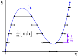
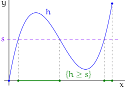
Figure 2. The lower Hadwiger integral is defined as a limit of lower step functions (left), as in Definition 6. It can also be expressed in terms of excursion sets (right), as in Theorem 7, equation (21).

5. Continuous valuations

Valuations on functions are a straightforward generalization of valuations on sets. A valuation on $\mathbf{Def}({}^{n})$ is a functional $v:\mathbf{Def}({}^{n})\to\real$, satisfying $v(0)=0$ and the following additivity condition:

(27) $$v(f)+v(g)=v(f\vee g)+v(f\wedge g),$$

where $\vee$ and $\wedge$ denote the pointwise max and min, respectively.

We present two useful topologies on $\mathbf{Def}({}^{n})$ that allow us to consider continuous valuations. With these topologies, the notion of a continuous valuation on $\mathbf{Def}({}^{n})$ properly extends the notion of a continuous valuation on definable subsets of ⁿ.

Definition 8.

Let $f,g,\in\mathbf{Def}({}^{n})$. The lower and upper flat metrics on definable functions, denoted $\underline{d}_{\flat}$ and $\overline{d}_{\flat}$, respectively, are defined as follows (see 13):

(28) $$\underline{d}_{\flat}(f,g) =\int_{-\infty}^{\infty}d_{\flat}(\mathbf{C}^{\{f\geq s\}},\mathbf{C}^{\{g\geq s\}})\ ds\quad\text{and}$$

(29) $$\overline{d}_{\flat}(f,g) =\int_{-\infty}^{\infty}d_{\flat}(\mathbf{C}^{\{f>s\}},\mathbf{C}^{\{g>s\}})\ ds.$$

The distinct topologies induced by the lower and upper flat metrics are the lower and upper flat topologies on definable functions. A valuation on definable functions is lower- or upper-continuous if it is continuous in the lower or upper flat topology, respectively.

Note that the integrals in (28) and (29) are well-defined because they may be written with finite bounds, as it suffices to integrate between the minimum and maximum values of $f$ and $g$. These metrics extend the flat metric on definable sets, for they reduce to (13) when $f$ and $g$ are characteristic functions.

Remark 9.

Definition 8 does result in metrics. If $\underline{d}_{\flat}(f,g)=0$, then $\left|\mathbf{C}^{\{f\geq s\}}-\mathbf{C}^{\{g\geq s\}}\right|_{\flat}=0$ only for $s$ in a set of Lebesgue measure zero. However, if the excursion sets of $f$ and $g$ agree almost everywhere, then all excursion sets of $f$ and $g$ agree, and thus $f=g$. For, if $\{s_{i}\}_{i}$ is a sequence of negative real numbers converging $0$, and $\{f\geq s_{i}\}=\{g\geq s_{i}\}$ for all $i$, then:

$$\{f\geq 0\}=\bigcap_{i}\{f\geq s_{i}\}=\bigcap_{i}\{g\geq s_{i}\}=\{g\geq 0\}.$$

The result for $\overline{d}_{\flat}(f,g)$ follows similarly from the observation that $\{f>0\}=\bigcup_{s>0}\{f>s\}$.

Remark 10.

That the lower and upper flat topologies are distinct can be seen by noting that for the identity function $f$ on the interval $[0,1]$, the sequence of lower step functions $g_{m}=\frac{1}{m}\left\lfloor mf\right\rfloor$ converges (as $m\to\infty$) to $f$ in the lower flat topology, but not in the upper flat topology. Dually, upper step functions converge in the upper flat topology, but not in the lower.

Lemma 11.

The lower and upper Hadwiger integrals are lower- and upper-continuous, respectively.

Proof.

Let $f,g\in\mathbf{Def}({}^{n})$ be supported on $X\subset{}^{n}$. The following inequality for the lower integrals is via (14):

$$\left|\int f{\lfloor d\mu_{k}\rfloor}-\int g{\lfloor d\mu_{k}\rfloor}\right| =\left|\int_{-\infty}^{\infty}(\mu_{k}\{f\geq s\}-\mu_{k}\{g\geq s\})\ ds\right|$$

$$\leq\int_{-\infty}^{\infty}\left|\left(\mathbf{C}^{\{f\geq s\}}-\mathbf{C}^{\{g\geq s\}}\right)\cap B^{*}_{1}{}^{n}\right|_{\flat}\cdot\max\left\{\sup_{B^{*}_{1}{}^{n}}|\omega|,\sup_{B^{*}_{1}{}^{n}}|d\omega|\right\}$$

$$=\underline{d}_{\flat}(f,g)\cdot\max\left\{\sup_{B^{*}_{1}{}^{n}}|\omega|,\sup_{B^{*}_{1}{}^{n}}|d\omega|\right\}$$

Since $\omega_{k}$ and $d\omega_{k}$ are bounded, we have continuity of the lower integrals in the lower flat topology. The proof for the upper integrals is analogous. ∎

For constructible functions, the lower and upper flat topologies of the previous section are equivalent. Thus, we may refer to the flat topology on constructible functions without specifying upper or lower. A valuation on constructible functions is conormal continuous if it is continuous with respect to the flat topology. Conormal continuity is the same as “smooth” in the Alesker sense [3, 4], but distinct from continuity in the topology induced by the Hausdorff metric on definable sets.

6. Hadwiger’s Theorem for functions

A dual pair of Hadwiger-type classifications for (lower-/upper-) continuous Euclidean-invariant valuations is the goal of this paper.

Lemma 12.

If $v:\mathbf{CF}({}^{n})\to\real$ is a (conormal) continuous valuation on constructible functions, invariant with respect to the right action by Euclidean motions, then $v$ is of the form:

$$v(h)=\sum_{k=0}^{n}\int_{{}^{n}}c_{k}(h)\ d\mu_{k}.$$

for some coefficient functions $c_{k}:\real\to\real$ with $c_{k}(0)=0$.

Proof.

For the class of indicator functions for convex sets $\{h=r\cdot{\mathbf{1}}_{A}:r\in{\mathbb{Z}}\text{ and }A\subset{}^{n}\text{ definable}\}$, continuity of $v$ in the flat topology implies that $v$ is continuous in the Hausdorff topology. Since convex tame sets are dense (in Hausdorff metric) among convex sets in ⁿ, Hadwiger’s Theorem for sets implies that

(30) $$v(r\cdot{\mathbf{1}}_{A})=\sum_{k=0}^{n}c_{k}(r)\mu_{k}(A),$$

where $c_{k}(r)$ are constants that depend only on $v$, not on $A$. Conormal continuity implies that the valuation $v(A)$ is the integral of the linear combination of the forms $\omega_{k}$ (defined in (12)),

(31) $$\sum_{k=0}^{n}c_{k}(r)\alpha_{k}$$

over $\mathbf{C}^{A}$.

Now suppose $h=\sum_{i=1}^{m}r_{i}{\mathbf{1}}_{A_{i}}$ is a finite sum of indicator functions of disjoint definable subsets $A_{1},\ldots,A_{m}$ of ⁿ for some integer constants $r_{1}<r_{2}<\cdots<r_{m}$. By equation (30) and additivity,

(32) $$v(h)=\sum_{k=0}^{n}\sum_{i=1}^{m}c_{k}(r_{i})\mu_{k}(A_{i}).$$

We can rewrite equation (32) in terms of excursion sets of $h$. Let $B_{i}=\bigcup_{j\geq i}A_{j}$. That is, $B_{i}=\{h\geq r_{i}\}$ and $B_{i}=\{h>r_{i-1}\}$. Then the valuation $v(h)$ can be expressed as:

(33) $$v(h)=\sum_{k=0}^{n}\sum_{i=1}^{m}\left(c_{k}(r_{i})-c_{k}(r_{i-1})\right)\mu_{k}(B_{i}),$$

where $c_{k}(r_{0})=0$. Thus, a valuation of a constructible function can be expressed as a sum of finite differences of valuations of its excursion sets. Equivalently, equation (33) can be written in terms of constructible Hadwiger integrals:

(34) $$v(h)=\sum_{k=0}^{n}\int_{{}^{n}}c_{k}(h)\ d\mu_{k}.$$

Since we require that a valuation of the zero function is zero, it must be that $c_{k}(0)=0$ for all $k$. ∎

Note that Lemma 12 holds for functions of the form $h=\sum_{i=1}^{m}r_{i}{\mathbf{1}}_{A_{i}}$ where the $A_{i}$ are definable and the $r_{i}\in\real$ are not necessarily integers.

In writing an arbitrary valuation on definable functions as a sum of Hadwiger integrals, the situation becomes complicated if the coefficient functions $c_{k}$ are decreasing on any interval. The following proposition illustrates the difficulty:

Proposition 13.

Let $c:\real\to\real$ be a continuous, strictly decreasing function. Then,

(35) $$\lim_{m\to\infty}\int_{{}^{n}}c\left(\frac{1}{m}\lceil mh\rceil\right)\ d\mu_{k}=\lim_{m\to\infty}\int_{{}^{n}}\frac{1}{m}\lfloor mc(h)\rfloor\ d\mu_{k}.$$

Proof.

On the left side of equation (35), we integrate $c$ composed with upper step functions of $h$:

$$\int_{{}^{n}}c\left(\frac{1}{m}\lceil mh\rceil\right)\ d\mu_{k}=\sum_{i\in{\mathbb{Z}}}c\left(\tfrac{i}{m}\right)\cdot\mu_{k}\left\{\tfrac{i-1}{m}<h\leq\tfrac{i}{m}\right\}.$$

On the right side of equation (35), we integrate lower step functions of the composition $c(h)$:

$$\int_{{}^{n}}\frac{1}{m}\lfloor mc(h)\rfloor\ d\mu_{k}=\sum_{t\in{\mathbb{Z}}}\tfrac{t}{m}\cdot\mu_{k}\left\{\tfrac{t}{m}\leq c(h)<\tfrac{t+1}{m}\right\}.$$

Since $c$ is strictly decreasing, $c^{-1}$ exists. There exists a discrete set

$$\mathcal{S}=\left\{c^{-1}\left(\tfrac{t}{m}\right)\ \big{|}\ t\in{\mathbb{Z}}\right\}\cap\{\text{neighborhood around range of $h$}\}.$$

We may then rewrite the above sum as:

$$\int_{{}^{n}}\frac{1}{m}\lfloor mc(h)\rfloor\ d\mu_{k}=\sum_{s\in\mathcal{S}}c(s)\cdot\mu_{k}\{c(s)\leq c(h)<c(s-\epsilon)\}=\sum_{s\in\mathcal{S}}c(s)\cdot\mu_{k}\{s-\epsilon<h\leq s\},$$

where $\epsilon\to 0$ as $m\to\infty$ by continuity of $c$. In the limit, both sides are equal:

$$\lim_{\epsilon\to 0}\sum_{s\in\mathcal{S}}c(s)\cdot\mu_{k}\{s-\epsilon<h\leq s\}\}=\lim_{m\to\infty}\sum_{i\in{\mathbb{Z}}}c\left(\tfrac{i}{m}\right)\cdot\mu_{k}\left\{\tfrac{i-1}{m}<h\leq\tfrac{i}{m}\right\}.\qed$$

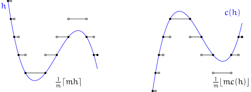
Figure 3. An upper step function of $h$, depicted at left, composed with a decreasing function $c$, becomes a lower step function of $c(h)$, depicted at right. As the step size approaches zero, we obtain Proposition 13.

Proposition 13 implies that if $c:\real\to\real$ is increasing on some interval and decreasing on another, then the maps $v,u:\mathbf{Def}({}^{n})\to\real$ defined

$$v(h)=\int_{{}^{n}}c(h){\lfloor d\mu_{k}\rfloor}\quad\text{and}\quad u(h)=\int_{{}^{n}}c(h){\lceil d\mu_{k}\rceil}$$

are neither lower- nor upper-continuous.

Lemma 12 and Proposition 13 provide a generalization of Hadwiger’s Theorem:

Theorem 14.

Any ${\mathbb{E}}_{n}$-invariant definably lower-continuous valuation $v:\mathbf{Def}({}^{n})\to\real$ is of the form:

(36) $$v(h)=\sum_{k=0}^{n}\left(\int_{{}^{n}}c_{k}\circ h{\lfloor d\mu_{k}\rfloor}\right)\,,$$

for some $c_{k}\in C(\real)$ continuous and monotone, satisfying $c_{k}(0)=0$. Likewise, an upper-continuous valuation can be similarly written in terms of upper Hadwiger integrals.

Proof.

Let $v:\mathbf{Def}({}^{n})\to\real$ be a lower valuation, and $h\in\mathbf{Def}({}^{n})$. First approximate $h$ by lower step functions. That is, for $m>0$, let $h_{m}=\frac{1}{m}\lfloor mh\rfloor$. In the lower flat topology, $\lim_{m\to\infty}h_{m}=h$. On each of these step functions, Lemma 12 implies that $v$ is a linear combination of Hadwiger integrals:

(37) $$v(h_{m})=\sum_{k=0}^{n}\int_{{}^{n}}c_{k}(h_{m})\ d\mu_{k}.$$

for some $c_{k}:\real\to\real$ with $c_{k}(0)=0$, depending only on $v$ and not on $m$. By Proposition 13, the $c_{k}$ must be increasing functions since we are approximating $h$ with lower step functions in the lower flat topology.

We can alternately express equation (37) as

(38) $$v(h_{m})=\sum_{k=0}^{n}\int_{{}^{n}}c_{k}(h_{m})\ {\lfloor d\mu_{k}\rfloor},$$

where we choose lower rather than upper integrals since $v$ is continuous in the lower flat topology. Continuity of $v$, and convergence of $h_{m}$ to $h$, in the lower flat topology imply that $v(h_{m})$ converges to $v(h)$ as $h\to\infty$. More specifically,

(39) $$v(h)=\lim_{m\to\infty}v\left(h_{m}\right)=\sum_{k=0}^{n}\lim_{m\to\infty}\int_{{}^{n}}c_{k}\left(h_{m}\right)\ {\lfloor d\mu_{k}\rfloor}.$$

By continuity of the lower Hadwiger integrals (Lemma 11) and the $c_{k}$, Equation (39) becomes

(40) $$v(h)=\sum_{k=0}^{n}\int_{{}^{n}}c_{k}\left(\lim_{m\to\infty}h_{m}\right)\ {\lfloor d\mu_{k}\rfloor}=\sum_{k=0}^{n}\int_{{}^{n}}c_{k}(h)\ {\lfloor d\mu_{k}\rfloor}.$$

The proof for the upper valuation is analogous. ∎

Corollary 15.

Any ${\mathbb{E}}_{n}$-invariant valuation both upper- and lower-continuous is a weighted Lebesgue integral.

Proof.

Integration with respect to ${\lfloor d\mu_{k}\rfloor}$ and ${\lceil d\mu_{j}\rceil}$ are independent unless $k=j=n$. For any $v$ both upper- and lower-continuous, we have

$$v(h)=\sum_{k=0}^{n}\int_{{}^{n}}\underline{c}_{k}(h)\ {\lfloor d\mu_{k}\rfloor}=\sum_{k=0}^{n}\int_{{}^{n}}\overline{c}_{k}(h)\ {\lceil d\mu_{k}\rceil}$$

for some functions $\underline{c}_{k}$ and $\overline{c}_{k}$.

Lower and upper Hadwiger integrals with respect to $\mu_{k}$ are unequal, except when $k=n$, implying that $\underline{c}_{k}=\overline{c}_{k}=0$ for $k=0,1,\ldots,n-1$, and $\underline{c}_{n}=\overline{c}_{n}$. Therefore,

$$v(h)=\int_{{}^{n}}c(h)\ d\mu_{n}$$

for some continuous function $c:\real\to\real$, and with $d\mu_{n}={\lfloor d\mu_{n}\rfloor}={\lceil d\mu_{n}\rceil}$ denoting Lebesgue measure. ∎

7. Speculation

The present constructions are potentially applicable to generalizations of current applications of intrinsic volumes. One such recent application is to the dynamics of cellular structures, such as crystals and foams in microstructure of materials. The cells in such structures often change shape and size over time in order to minimize the total energy level in the system. Let $C=\bigcup_{i=0}^{n}C_{i}$ be a closed $n$-dimensional cell, with $C_{i}$ denoting the union of all $i$-dimensional features of the cell: i.e., $C_{0}$ is the set of vertices, $C_{1}$ the set of edges, etc. MacPherson and Srolovitz found that when the cell structure changes by a process of mean curvature flow, the volume of the cell changes according to

(41) $$\frac{d\mu_{n}}{dt}(C)=-2\pi M\gamma\left(\mu_{n-2}(C_{n})-\frac{1}{6}\mu_{n-2}(C_{n-2})\right)$$

where $M$ and $\gamma$ are constants determined by the material properties of the cell structure [22]. Replacing the intrinsic volumes of cells with Hadwiger integrals may (1) lead to interesting dynamical systems on the (singular) foliations (by the level sets of a piece-wise smooth function, and (2) allow for description of evolution of real-valued physical fields (temperature, density, etc.) of cells.

A more widely-known application of the intrinsic volumes is in the formulas for expected Euler characteristic of excursion sets in Gaussian random fields [1, 2]. These formulae and the associated Gaussian kinematic formula [2] rely crucially on the intrinsic volumes of excursion sets. It is already recognized in recent work [8] that the definable Euler measure ${\lfloor d\chi\rfloor}={\lfloor d\mu_{0}\rfloor}$ is relevant to Gaussian random fields: we strongly suspect that the other definable Hadwiger measures ${\lfloor d\mu_{k}\rfloor}$ and ${\lceil d\mu_{k}\rceil}$ of this paper are immediately applicable to Gaussian random fields.

References

- [1] R. Adler, The Geometry of Random Fields, Wiley, 1981; reprinted by SIAM, 2009.
- [2] R. Adler and J. Taylor, “Topological Complexity of Random Functions”, Springer Lecture Notes in Mathematics, Vol. 2019, Springer, 2011.
- [3] S. Alesker, “Theory of valuations on manifolds: a survey,” Geometric and Functional Analysis, 17(4), 2007, 1321–1341.
- [4] S. Alesker, “Valuations on manifolds and integral geometry,” Geometric and Functional Analysis, 20(5), 2010, 1073–1143.
- [5] A. Bernig, “Algebraic Integral Geometry,” Global Differential Geometry, edited by C Bär, J. Lohkamp, and M. Schwarz, Springer, 2012.
- [6] Y. Baryshnikov and R. Ghrist, “Target enumeration via Euler characteristic integration,” SIAM J. Appl. Math., 70(3), 2009, 825–844.
- [7] Y. Baryshnikov and R. Ghrist, “Definable Euler integration,” Proc. Nat. Acad. Sci., 107(21), May 25, 9525-9530, 2010.
- [8] O. Bobrowski and M. Strom Borman, “Euler Integration of Gaussian Random Fields and Persistent Homology,” 2011, arXiv:1003.5175.
- [9] J. Cheeger, W. Müller, and R. Schrader, “On the curvature of piecewise flat spaces,” Comm. Math. Phys. 92(3), 1984, 405–454.
- [10] M. Coste, An Introduction to o-minimal Geometry, Dip. Mat. Univ. Pisa, Dottorato di Ricerca in Matematica, Istituti Editoriali e Poligrafici Internazionali, Pisa, 2000, http://www.ihp-raag.org/publications.php.
- [11] H. Federer, Geometric Measure Theory, Springer 1969.
- [12] J. Fu, “Curvature measures of subanalytic sets”, Amer. J. Math., 116, (1994), 819-890.
- [13] J. Fu, “Notes on Integral Geometry,” 2011, http://www.math.uga.edu/~fu/notes.pdf.
- [14] R. Ghrist and M. Robinson, “Euler-Bessel and Euler-Fourier transforms,” Inv. Prob., to appear.
- [15] Guesin-Zade, “Integration with respect to the Euler characteristic and its applications,” Russ. Math. Surv., 65:3, 2010, 399–432.
- [16] H. Hadwiger, “Integralsätze im Konvexring,” Abh. Math. Sem. Hamburg, 20, 1956, 136–154.
- [17] D. A. Klain and G.-C. Rota, Introduction to Geometric Probability, Cambridge, 1997.
- [18] M. Kashiwara, “Index theorem for constructible sheaves,” Ast risque, 130, 1985, 193–209.
- [19] D. A. Klain, “A Short Proof of Hadwiger’s Characterization Theorem,” Mathematika, 42, 1995, 329–339.
- [20] M. Kashiwara and P. Schapira, Sheaves on Manifolds, Springer, 1990.
- [21] M. Ludwig, “Valuations on function spaces,” Adv. Geom., 11, (2011), 745–756.
- [22] R. D. MacPherson and D. J. Srolovitz, “The von Neumann relation generalized to coarsening of three-dimensional microstructures,” Nature, 446, 2007, 1053–1055.
- [23] L. I. Nicolaescu, “Conormal Cycles of Tame Sets,” preprint, 2010, http://www.nd.edu/~lnicolae/conormal.pdf.
- [24] L. I. Nicolaescu, “On the Normal Cycles of Subanalytic Sets,” Ann. Glob. Anal. Geom. 39, 2011, 427–454.
- [25] P. Schapira, “Operations on constructible functions,” J. Pure Appl. Algebra, 72, 1991, 83–93.
- [26] J. Schürmann, Topology of Singular Spaces and Constructible Sheaves, Birkhäuser, 2003.
- [27] S. H. Schanuel, “What is the Length of a Potato?” in Lecture Notes in Mathematics, Springer, 1986, 118–126.
- [28] M. Shiota, Geometry of subanalytic and semialgebraic sets, Birkhäuser, 1997.
- [29] L. Van den Dries, Tame Topology and O-Minimal Structures, Cambridge University Press, 1998.