Collective charge fluctuations and Casimir interactions
for quasi one-dimensional metals

Abstract

We investigate the Casimir interaction between two parallel metallic cylinders and between a metallic cylinder and plate. The material properties of the metallic objects are implemented by the plasma, Drude and perfect metal model dielectric functions. We calculate the Casimir interaction numerically at all separation distances and analytically at large separations. The large-distance asymptotic interaction between one plasma cylinder parallel to another plasma cylinder or plate does not depend on the material properties, but for a Drude cylinder it depends on the dc conductivity $\sigma$. At intermediate separations, for plasma cylinders the asymptotic interaction depends on the plasma wave length $\lambda_{\rm p}$ while for Drude cylinders the Casimir interaction can become independent of the material properties. We confirm the analytical results by the numerics and show that at short separations, the numerical results approach the proximity force approximation.

I Introduction

Effective interactions between cylinders are an important parameter in synthesizing and analyzing nanometric systems. This is due to the fact that many important nanostructures such as carbon nanotubes, nanowires and even the tobacco mosaic viruses have cylinderical shapes.

From the perspective of the experimental Casimir force studies, nano-cylindrical shapes are an optimal candidate for precision Casimir force measurements, in comparison to spheres for two reasons: (i) their effective area of interaction is larger Brown-Hayes et al. (2005); Decca et al. (2010), and (ii) mechanical oscillation modes of quasi-one-dimensional structures can be probed with high precision Sazonova et al. (2004).

Under many circumstances, van der Waals or Casimir forces have the dominant contribution in the effective interactions of nanostructures, which lead to various interesting phenomena in nanosystesm. For example in nanomechanical devices, Casimir interaction causes stiction Serry et al. (1998); Buks and Roukes (2001), and thus a good understanding of these forces leads to improvements in the design and efficiency of such nanosystems. In another example, Casimir interactions between single walled carbon nanotubes (SWCNT) with different chirality become important in separating a polydisperse solution of SWCNT in fractions of equal chirality Šiber et al. (2009).

The applicability of the Casimir interaction is not limited to synthetic cylindrical objects. There are numerous examples of long macromolecular structures with cylindrical shape in nature such as the tobacco mosaic viruses, microtubules of flagella and A-band lattice of myosin filaments in cross strained muscles Elliott (1968); Parsegian (1972), and hence knowledge of the interaction between cylindrical shapes is also important for the biological sciences. It should be noted that in some biological systems composed of cylindrical particles which are packed in an array, the separation between the particles can be several times larger than the diameter of the cylinder Elliott (1968).

The Casimir interaction per unit length for two parallel perfectly conducting cylinders or a plate and cylinder at a separation distance $d$ is ${\cal E}/L\sim\hbar c/d^{2}$, up to a logarithmic factor Emig et al. (2006); Rahi et al. (2008). It decays only slowly compared to the retarded interaction ${\cal E}/L\sim\hbar cR^{4}/d^{6}$ between two insulating cylinders that do not support large-scale collective fluctuations Rahi et al. (2009).

It has been demonstrated that Casimir interactions strongly depend on the combined effects of shape and material properties, see, e.g., U. Mohideen and Mostepanenko (2009); Emig et al. (2009); Graham et al. (2010); Maghrebi et al. (2011); Zandi et al. (2010); Noruzifar et al. (2011). The interplay is particularly strong for quasi one-dimensional conducting materials due to strongly anisotropic collective charge fluctuations. In addition, approximations of the Casimir force between cylinders and plates Decca et al. (2010) have also shown that the temperature dependence varies based on the description of the material properties. Thus there is a need for exact calculations of the Casimir force for cylindrical shapes taking into account the realistic material response.

Most studies of interactions between one-dimensional systems over a wide range of separations concentrate on perfect conductors and insulators. However, low dimensionality in combination with finite conductivity and plasmon excitations should give rise to interesting new effects that might be probed experimentally using, e.g., the coupling to mechanical oscillation modes. The often employed technique for these effects, the proximity force approximation (PFA) cannot capture the correlations of shape and material response since it is based on the interaction between planar surfaces. A number of studies have been performed for the short separation regime mainly focused on the corrections to the Proximity Force Approximation Bordag et al. (2006); Bordag (2006); Lombardo et al. (2008); Weber and Gies (2010).

Van der Waals interaction between cylinders (and plates) have been studied for certain frequency dependent permittivities Barash and Kyasov (1989); Dobson et al. (2006); Mazzitelli et al. (2006); Emig et al. (2006); Rahi et al. (2008); Drummond and Needs (2007); Dobson et al. (2009). In one of the earliest study, the van der Waals interaction has been calculated between two parallel thin filaments described by one dimensional (1D) plasmon and electromagnetic excitations Barash and Kyasov (1989). This work predicts asymptotic forms of the interaction energies at large separations accurately but the range of validity of the asymptotics remain unclear.

In another work Dobson et al. (2006), the Casimir interaction is obtained for conducting cylinders described by delocalized coupled 1D plasmons at zero temperature. The response function of the plasmons are given by the random phase approximation (RPA). The specific choice of RPA has the advantage that locality, additivity and $R^{-6}$ contributions are not involved in the calculations. The energy is obtained by using the mode summation method, which is equal to the sum of the separation dependent zero-point plasmon modes. The Casimir energy is attractive and decays as $\sim d^{-2}$ apart from a logarithmic part. This result was later confirmed by a quantum Monte Carlo simulation Drummond and Needs (2007). Using the same material description and calculation technique, the large-distance Casimir energy was obtained for crossed wires with a small crossing angle. For conducting and semiconductor wires, apart from the logarithmic and angular parts, the large-distance interaction energy decays as $\sim d^{-1}$ and $\sim d^{-4}$, respectively Dobson et al. (2009).

In a completely different approach, employed for perfectly conducting cylinders and plate, the Casimir energy is calculated for all separations using a path integral representation for the effective action which yields a trace formula for the density of states Emig et al. (2006); Rahi et al. (2008). Furthermore, the Casimir interaction between a SWCNT and a plate is studied for large and short separation regimes using the Lifshitz formula Bordag et al. (2006).

The full interplay between shape and material effects is not transparent in the previous studies as they are limited either to perfect metals or to asymptotic limits. Here, we employ the scattering approach to investigate the Casimir interaction between parallel metallic (circular) cylinders, and a metallic cylinder and a metallic plate. The material properties of the objects are described either by the plasma or the Drude dielectric function. Some of the results have been reported in Ref. Noruzifar et al. (2011).

The outline of this work is as follows: in Sec. II, we summarize the scattering method and the assumed material properties of the cylinders. In Sec. III, we obtain analytical results for the interaction at distances much larger than the cylinder radii. In Sec. IV the Casimir interaction is calculated numerically for different material properties over a wide range of separations. Section V is the summary.

II Method

We consider the two following systems (i) two infinitely long parallel cylinders, and (ii) an infinitely long cylinder parallel to an infinite plate. Assuming placed in vacuum, we calculate the Casimir interaction in these two systems employing the scattering formalism Rahi et al. (2009). The Casimir energy of two objects at zero temperature is given by the general expression

$${\cal E}=\frac{\hbar c}{2\pi}\int_{0}^{\infty}d\kappa\,\ln\det({\bf 1}-\mathbb{N})\,,$$ (1)

where $\kappa$ is the Wick-rotated frequency and the matrix $\mathbb{N}$ factorizes into the scattering amplitudes (T-matrices) and translation matrices that describe the coupling between the multipoles on distinct objects. While the material properties and shapes of the objects are contained in the T-matrices, the distance between objects is encoded in translation matrices.

To implement the material properties, we consider plasma, Drude and perfect metal cylinders with magnetic permeability $\mu=1$. The Drude dielectric function on the imaginary frequency axis is

$$\epsilon(ic\kappa)=1+\frac{(2\pi)^{2}}{(\lambda_{\rm p}\kappa)^{2}+\lambda_{\sigma}\kappa/2}\,,$$ (2)

with conductivity $\sigma$ and $\lambda_{\sigma}=2\pi c/\sigma$. Equation (2) reproduces the plasma model for $\lambda_{\sigma}\to 0$.

Since the matrix $\mathbb{N}$ differs for parallel cylinders and cylinder-plate systems, in the following we describe $\mathbb{N}$ for both setups.

II.1 Two Parallel Cylinders

Consider two infinitely long, parallel cylinders with equal radii $R$ and with their axes separated by a distance $d$ and aligned along the $z$-axis. The matrix $\mathbb{N}$ is diagonal in the $z$-component $k_{z}$ of the wave vector due to translational symmetry. The matrix elements for electric (E) and magnetic (M) polarizations ($\alpha,~{}\beta=E,~{}M$) and partial waves $m$ and $m^{\prime}$ are

$${\mathbb{N}}_{k_{z}mm^{\prime}}^{\alpha\beta}=\sum_{\gamma=E,M}T_{k_{z}m}^{\alpha\gamma}\sum_{n=-\infty}^{\infty}{\mathcal{U}}_{k_{z}mn}^{12}T_{k_{z}n}^{\gamma\beta}{\mathcal{U}}_{k_{z}nm^{\prime}}^{21}\,,$$ (3)

with $T$ the cylinder $T$-matrix, see Appendix A.1. The translation matrix ${\mathcal{U}}^{12}$ relates regular cylindrical vector waves to outgoing cylindrical vector waves, see Appendix B. The translation matrices do not couple different polarizations and for both $E$ and $M$-polarization, their matrix elements are given by

$${\mathcal{U}}^{12}_{k_{z}nn^{\prime}}=(-1)^{n^{\prime}}\,K_{n-n^{\prime}}\left(p\,d\right),$$

$${\mathcal{U}}^{21}_{k_{z}nn^{\prime}}=(-1)^{n-n^{\prime}}\,{\mathcal{U}}^{12}_{k_{z}nn^{\prime}}\;,$$ (4)

with $p=\sqrt{\kappa^{2}+k_{z}^{2}}$ and $K_{n}(x)$ the modified Bessel function of the second kind.

Since $\mathbb{N}$ is diagonal in $k_{z}$ the determinant in Eq. (1) factorizes into determinants at fixed $k_{z}$, and the sum over $k_{Z}$ moves in front of the logarithm. After taking the continuum limit, $\sum_{k_{z}}\to\frac{L}{2\pi}\int_{-\infty}^{\infty}dk_{z}$, the energy per unit length $L$ becomes

$$\frac{{\cal E}}{L}=\frac{\hbar c}{4\pi^{2}}\int_{0}^{\infty}d\kappa\int_{-\infty}^{\infty}dk_{z}\ln\det({\bf 1}-\mathbb{N})\,.$$ (5)

Here the determinant is only over the discrete partial wave index $n$.

II.2 Cylinder – Plate

Next we consider a cylinder with radius $R$ parallel to a plate. We assume that the cylinder is aligned along the $z$ axis and the plate is in the $y-z$ plane. The distance from the center of the cylinder to the plate is $d$. The matrix $\mathbb{N}$ for this geometry is

$$\mathbb{N}_{k_{z}mm^{\prime}}^{\alpha\beta}=\sum_{\gamma=E,M}{{T}}_{k_{z}m}^{\alpha\gamma}\,{\mathbb{M}_{k_{z}mm^{\prime}}^{\gamma\beta}}\,,$$ (6)

with

$$\mathbb{M}_{k_{z}mm^{\prime}}^{\gamma\beta}=\int_{-\infty}^{\infty}dk_{y}\,\frac{e^{-2d\sqrt{{\bf k}_{\bot}^{2}+\kappa^{2}}}}{2\sqrt{{\bf k}_{\bot}^{2}+\kappa^{2}}}\\ \times\sum_{\gamma^{\prime}=E,M}D_{k_{z}m\gamma,{\bf k}_{\bot}\gamma^{\prime}}\;T^{\gamma^{\prime}}_{{\bf k}_{\bot}}\;D_{{\bf k}_{\bot}\gamma^{\prime},k_{z}m^{\prime}\beta}^{\dagger}\;(1-2\delta_{\gamma^{\prime},\beta})\,,$$ (7)

where $k_{y}$ is the $y$ component of the wave vector, ${\bf k_{\bot}}\equiv(k_{y},k_{z})$, the matrix ${D}_{nk_{z}\alpha,{\bf k}_{\bot}\beta}$ converts vector plane wave functions and cylindrical vector wave functions, see Appendix C, and $T^{\beta}_{{\bf k}_{\bot}}$ is the dielectric plane $T$-matrix presented in Appendix A.2. The energy of this system can also be obtained by Eq. (5) as $\mathbb{N}$ is diagonal in $k_{z}$, Note that the determinant is not related to $k_{z}$; thus, we suppress all the $k_{z}$ indices in what follows.

III large-distance asymptotic Casimir energies

To find the asymptotic form of the Casimir interaction at large separations $d\gg R$, one needs to obtain the T-matrix expressions for a cylinder and a plate. Using the dielectric function given in Eq. (2), the asymptotic form of the cylinder T-matrix elements for $E$ polarization and $n=0$ at small frequencies ($\kappa\ll 1$, $k_{z}/\kappa$ fixed) reads (see Eq. (43)),

$$T_{0}^{EE}\approx-\frac{p^{2}R^{2}}{C(\kappa)-p^{2}R^{2}\ln(pR/2)}\,,$$ (8)

where $C(\kappa)$ depends on the dielectric properties of the cylinder. For a perfect metal cylinder $C(\kappa)=0$ and for a plasma cylinder $C(\kappa)\approx{\lambda_{\rm p}}^{2}\kappa^{2}\,/(2\pi^{2})$ if the plasmon oscillations cannot build up transverse to the cylinder axis as the diameter is too small, i.e., $R\ll\lambda_{p}$. In the opposite limit $R\gg\lambda_{p}$, we reproduce the perfect metal form of the T-matrix, i.e. $C(\kappa)\approx 0$. For the Drude model, $C(\kappa)={\lambda_{\sigma}\kappa}/{(4\pi^{2})}$ if $\kappa\ll\lambda_{\sigma}/\lambda_{p}^{2}$, $1/\lambda_{\sigma}$. The first of the two conditions implies that Drude behavior dominates over plasma behavior, i.e., the second term in the denominator of Eq. (2) is larger than the first term. The second condition ensures that the Drude dielectric function is large compared to one, i.e., metallic behavior is pronounced. At small frequencies $\kappa$ but fixed $k_{z}/\kappa$, for Drude cylinders $T^{EE}_{0}\sim\kappa$, while for plasma and perfect metal cylinders $T^{EE}_{0}\sim 1$. Since $T^{MM}_{0}\sim\kappa^{2}$, $T^{EM}_{0}=T^{ME}_{0}=0$ and higher order elements associated with $n\neq 0$ scale as $\kappa^{2|n|}$, we consider only the $T_{0}^{EE}$ elements at large separations.

The Casimir interaction between conducting cylinders is intricate and no simple analytical expression that applies to all distances can be obtained. However, using Eqs. (5), (3) and (6) along with $T_{0}^{EE}$ given in Eq. (8), the asymptotic interaction at large separations, $d\gg R$, can be evaluated in various limiting cases.

To derive the large-distance asymptotic Casimir potential energy, we employ the identity $\log\det={\rm Tr}\log$ and expand the integrand in Eq. (5) in powers of $\mathbb{N}$, corresponding to a multiple scattering expansion. The one-scattering approximation, sufficient for large distances, yields

$$\frac{\mathcal{E}}{L}=-\frac{\hbar c}{4\pi^{2}}\int_{0}^{\infty}d\kappa\int_{-\infty}^{\infty}dk_{z}\,{\rm Tr}[\mathbb{N}]+...\,.$$ (9)

The element $\mathbb{N}_{00}$ of the $\mathbb{N}$-matrix yields the dominant contribution to the Casimir energy at large distances since higher order elements involve higher powers of $\kappa$. To this end, we will consider only this term for the rest of this section.

III.1 Parallel cylinders

For two parallel cylinders, considering the fact that at large separations $T^{EE}_{0}$ yields the dominant contribution, the trace of the matrix $\mathbb{N}$ is approximated by

$${\rm Tr}[\mathbb{N}{{}^{EE}_{00}}]=T^{EE}_{0}\,{\mathcal{U}}_{00}^{12}\,T^{EE}_{0}\,{\mathcal{U}}_{00}^{21}\,.$$ (10)

Using Eq. (10) in Eq. (9) and changing integration to polar coordinates $\kappa=\rho\cos(\theta)/d$ and $k_{z}=\rho\sin(\theta)/d$, we obtain

$${\mathcal{E}}=-\frac{\hbar cL}{2\pi^{2}d^{2}\ln^{2}(2d/R)}\\ \times\int_{0}^{\infty}d\rho\int_{0}^{\frac{\pi}{2}}d\theta\,\frac{\rho K_{0}^{2}(\rho)}{(1+C_{1}(\rho,\theta))(1+C_{2}(\rho,\theta))}\,,$$ (11)

where $C_{i}(\rho,\theta)$ describes the material properties of the cylinder $i$. For a perfect metal cylinder $C_{i}(\rho,\theta)=0$, for a plasma cylinder $C_{i}(\rho,\theta){=}\xi\cos^{2}(\theta)$ with

$$\xi=\frac{\lambda_{\rm p}^{2}}{2\pi^{2}R^{2}\ln(2d/R)}\,,$$ (12)

in the limit $R\ll\lambda_{p}$, and for a Drude cylinder $C_{i}(\rho,\theta)=\xi^{\prime}\cos(\theta)/\rho$ with

$$\xi^{\prime}=\frac{\lambda_{\sigma}d}{4\pi^{2}R^{2}\ln(2d/R)}.$$ (13)

For two perfect metal cylinders the integral in Eq. (11) can easily be calculated and yields

$$\frac{{\mathcal{E}}}{\hbar cL}\approx-\frac{1}{8\pi d^{2}\ln(2d/R)^{2}}\,,$$ (14)

which agrees with the results in Refs. Emig et al. (2006); Rahi et al. (2008).

For plasma cylinders with plasma wave length $\lambda_{\rm p}$, the integrations in Eq. (11) yield

$$\frac{{\mathcal{E}}}{L}\approx-\frac{\hbar c}{16\pi d^{2}\ln(2d/R)^{2}}f({\xi})\,,$$ (15)

with

$$f(x)=\frac{x+2}{(x+1)^{3/2}}\,.$$ (16)

It is important to consider Eq. (15) in two limiting cases for $\xi$, Eq. (12). In the limit $\xi\ll 1$ or $\ln(2d/R)\gg\lambda_{\rm p}^{2}/R^{2}$, the energy simplifies to the perfect metal energy given in Eq. (14), i.e., the interaction between conducting cylinders is universal at large distances in this regime. However, in the opposite limit $\xi\gg 1$ or equivalently $\ln(2d/R)\ll\lambda_{\rm p}^{2}/R^{2}$, the Casimir energy becomes

$$\frac{{\mathcal{E}}}{L}\approx-\frac{\hbar c\,R}{8\sqrt{2}\,\lambda_{\rm p}\,d^{2}\ln^{3/2}(2d/R)}\,.$$ (17)

This shows that the universal form is applicable only beyond an exponentially large crossover length $d\sim R\exp(\lambda_{\rm p}^{2}/R^{2}){\gg\!\!\gg R}$. Below this scale, and infact in any practical situations, the interaction is material dependent, see Fig. (1)a.

For a plasma cylinder with plasma wave length $\lambda_{\rm p}$ parallel to a perfect metal cylinder the integrations in Eq. (11) yield

$$\frac{{\mathcal{E}}}{L}\approx-\frac{\hbar c}{8\pi d^{2}\ln(2d/R)^{2}}(1+\xi)^{-{{1}\over{2}}}\,.$$ (18)

Similar to parallel plasma cylinders, we consider two limiting cases for $\xi$. In the limit $\xi\ll 1$ or $\ln(2d/R)\gg\lambda_{\rm p}^{2}/R^{2}$, we obtain the perfect metal energy given in Eq. (14), and the conducting cylinders’ interaction is universal at large distances. In the opposite limit $\xi\gg 1$ or equivalently $\ln(2d/R)\ll\lambda_{\rm p}^{2}/R^{2}$, the Casimir energy becomes

$$\frac{{\mathcal{E}}}{L}\approx-\frac{\hbar c\,R}{4\sqrt{2}\,\lambda_{\rm p}\,d^{2}\ln^{3/2}(2d/R)}\,.$$ (19)

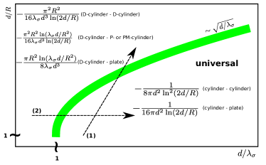
Figure 1: Summary of the different forms of interaction between two cylinders and a cylinder and a plate. Shown are the rescaled interaction energies per cylinder length, ${\cal E}/(\hbar cL)$. (a) Interaction involving a plasma (P) cylinder with another plasma cylinder, a perfect metal (PM) cylinder or a plate. The asymptotic results apply sufficiently far away from the separating curve $\ln(d/R)\sim(\lambda_{p}/R)^{2}$ and for $d/R$, $\lambda_{p}/R\gg 1$. (b) Interaction involving a Drude (D) cylinder with another Drude cylinder, a plasma cylinder, a perfect metal cylinder or a plate. The separating curve is given, up to logarithmic corrections, by $d/R\sim\sqrt{d/\lambda_{\sigma}}$. The shown expressions hold for $d/R$, $d/\lambda_{\sigma}\gg 1$ and $d\gg\lambda_{p}^{2}/\lambda_{\sigma}$. Depending on the relative size of length scales, different regimes can be reached: Arrow (1) corresponds to an increasing distance $d$ which ultimately leads to a non-universal interaction. Arrow (2) indicates an overall increase of the geometry (i.e., $d/R$ fixed) with constant conductivity leading to a universal interaction.

For Drude cylinders with the characteristic length $\lambda_{\sigma}$, at large separations $d\gg R,\,\lambda_{\sigma}$, we find a rather distinct behavior that deviates from naive expectations for universality. In this case the integrations in Eq. (11) cannot be performed analytically. Therefore we first calculate the angular integral which gives a complicated radial function, and then we expand the resulting radial integral for small and large $\xi^{\prime}$, Eq. (13). The radial integrals can be calculated easily in these two limits. For $\xi^{\prime}\ll 1$ or $d\ll R^{2}/\lambda_{\sigma}$, we reproduce the universal (perfect metal) asymptotic energy of Eq. (14). In the opposite limit $\xi^{\prime}\gg 1$ or $d\gg R^{2}/\lambda_{\sigma}$, the asymptotic energy reads

$$\frac{\mathcal{E}}{L}\approx-\frac{\pi^{2}\,\hbar c\,R^{2}}{16\,\lambda_{\sigma}\,d^{3}\ln(2d/R)}\,.$$ (20)

Similarly, for a Drude cylinder with the characteristic length $\lambda_{\sigma}$ parallel to a plasma (or perfect metal) cylinder, in the limit of $d\gg\lambda_{\sigma}$ and $d\gg\lambda_{\rm p}^{2}/\lambda_{\sigma}$ the asymptotic Casimir energy is

$$\frac{\mathcal{E}}{L}\approx-\frac{\pi^{2}\,\hbar c\,R^{2}}{16\,\lambda_{\sigma}\,d^{3}\ln(2d/R)}\ln(\lambda_{\sigma}\,d/R^{2})\,.$$ (21)

These two limiting cases for $\xi^{\prime}$ are related to two different scaling regimes that are separated, up to logarithmic corrections, by the curve $d/R\sim\sqrt{d/\lambda_{\sigma}}$, see Fig. 1(b). The unconventional feature corresponds to the fact that the interaction is universal at shorter distances where $d\ll R^{2}/\lambda_{\sigma}$. If the distance is increased beyond this crossover scale (with all other length scales kept fixed, see arrow (1) in Fig. 1(b), the interaction becomes material dependent and, up to logarithmic corrections, scales as $R^{2}/(\lambda_{\sigma}d^{3})$ for a Drude cylinder interacting with another Drude or a plasma or a perfect metal cylinder. However, if the radii of the cylinders are increased in the same way as their distance ($d/R$ fixed, see arrow (2) in Fig. 1(b)), finite conductivity becomes unimportant at large distances and the interaction assumes the universal form. An intuitive explanation of this non-universal large distance behavior is given below. It is important to note that all forms of these metallic interactions decay much slower than the Casimir energy of two insulating cylinders which for $d\gg R$ scales as $\hbar cLR^{4}/d^{6}$ with a material dependent coefficient.

III.2 Cylinder parallel to a plate

In this section we consider a cylinder with radius $R$ parallel to a plate. We show, similar to parallel cylinders, the existence of two different scaling regimes that are separated by curves given by the same expressions that we found for two cylinders, see Fig. 1. In order to find the asymptotic large distance interations, we employ again Eq. (9). The trace of the matrix $\mathbb{N}$ in Eq. (6) in the limit of large separation $d\gg R$ is approximated by

$${\rm Tr}[\mathbb{N}{{}^{EE}_{00}}]={T}^{EE}_{0}\mathbb{M}^{EE}_{00}\,.$$ (22)

Note that for perfect metal plates $T^{E}_{{\bf k}_{\bot}}=T^{M}_{{\bf k}_{\bot}}=1$ and for small $\kappa$ at fixed $k_{\perp}/\kappa$ one has for the plasma model $T^{E}_{{\bf k}_{\bot}}=T^{M}_{{\bf k}_{\bot}}=1+{\cal O}(\lambda_{p}\kappa)$ and for the Drude model $T^{E}_{{\bf k}_{\bot}}=T^{M}_{{\bf k}_{\bot}}=1+{\cal O}(\lambda_{\sigma}\kappa)$. Therefore, at large distances the material desription of the plate is unimportant and to leading order in $R/d$ one gets

$${\mathbb{M}}^{EE}_{00}\approx\int_{-\infty}^{\infty}dk_{y}\;\frac{e^{-2d\sqrt{\kappa^{2}+{\bf k}_{\bot}^{2}}}}{2\sqrt{\kappa^{2}+{\bf k}_{\bot}^{2}}}{=}K_{0}(2pd)\,.$$ (23)

Using Eq. (22) in Eq. (9), and changing again considering $\kappa=\rho\cos(\theta)/d$ and $k_{z}=\rho\sin(\theta)/d$, we obtain

$$\frac{\mathcal{E}}{L}=-\frac{\hbar c}{2\pi^{2}d^{2}\ln(2d/R)}\int_{0}^{\infty}d\rho\int_{0}^{\pi\over 2}d\theta\,\frac{\rho\,K_{0}(2\rho)}{1+C(\rho,\theta)}\,,$$ (24)

where the functions $C(\rho,\theta)\equiv C_{i}(\rho,\theta)$ are given by the expressions below Eq. (11)

For a perfect metal cylinder, the integrals can be calculated in a straight forward manner, resulting in the universal energy

$$\frac{\mathcal{E}}{L}=-\frac{\hbar c}{16\,\pi\,d^{2}\ln(2d/R)}\,.$$ (25)

For a plasma cylinder with the plasma wavelength $\lambda_{\rm p}$, after performing the radial and angular integrals in Eq. (24), we obtain

$$\frac{\mathcal{E}}{L}=-\frac{\hbar c}{16\,\pi\,d^{2}\ln(2d/R)}\;g({\xi})\,,$$ (26)

with $g(x)=(1+x)^{-1/2}$. As in our analysis for parallel cylinders we consider two different cases for $\xi$ given in Eq. (12). If $\xi\ll 1$ or similarly $\ln(2d/R)\gg\lambda_{\rm p}^{2}/R^{2}$, we reproduce the universal energy, Eq. (25). In the opposite limit of exponentially large distances $\xi\gg 1$ or $d\gg R\exp(\lambda_{\rm p}^{2}/R^{2})$ the Casimir energy is non-universal and we obtain

$$\color[rgb]{0,0,0}\frac{\mathcal{E}}{L}=-\frac{\hbar c\,R}{8\sqrt{2}\,\lambda_{\rm p}\,d^{2}\ln^{1/2}(2d/R)}\,.$$ (27)

For a Drude cylinder with the characteristic length $\lambda_{\sigma}$ parallel to a metallic plate, in the limit $\xi^{\prime}\ll 1$ or $d\ll R^{2}/\lambda_{\sigma}$, the integrand in Eq. (24) becomes independent of $\theta$ and we reproduce the universal Casimir energy in Eq. (25). Hence, similar to the case of two cylinders, the interaction approaches a universal form below a geometry and material dependent crossover distance. This counterintuitive result shall be discussed below. In the opposite limit $\xi^{\prime}\gg 1$ or $d\gg R^{2}/\lambda_{\sigma}$, the asymptotic energy becomes non-universal and reads

$$\frac{\mathcal{E}}{L}=-\frac{\pi\,\hbar c\,R^{2}\ln(\lambda_{\sigma}\,d/R^{2})}{8\,\lambda_{\sigma}\,d^{3}}\,.$$ (28)

Based on the studies described above, we conclude that the Casimir interaction between a metallic cylinder and a plate decays slower than that between an insulating cylinder and a plane for which the energy scales as ${\cal E}\sim\hbar cLR^{2}/d^{4}$ for $d\gg R$ Rahi et al. (2009).

IV Numerical Results

In this section, we compute the Casimir energy based on Eq. (5) at zero temperature. Our results are obtained by numerical computation of the determinant and the integrals over $\kappa$ and $k_{z}$. Note that for a cylinder parallel to a plate in addition to the $\kappa$ and $k_{z}$ integrations, one has to compute the integral over $k_{y}$ for each element of the matrix $\mathbb{N}$, see Eqs. (6) and (7). The matrix $\mathbb{N}$ (and hence the sum over $n$ in Eq. (3)) are truncated at a finite partial wave number $n_{\rm max}$.

We chose $n_{\rm max}$ such that the result for the energy changes by less than $0.01\%$ upon increasing $n_{\rm max}$ by $10$. The required value of $n_{\rm max}$ diverges when the surface-to-surface separation $h$ between the objects (for cylinders $h=d-2R$ and for a cylinder and a plate $h=d-R$) tends to zero. For example, for $0.6<h/R<1.0$, we used $n_{\rm max}=21$, whereas for $h/R=0.6$ and $0.5$, one needs $n_{\rm max}=31$. For $h/R=0.05$ we set the value $n_{\rm max}=191$. .

To reach sufficient numerical accuracy in the computation of $\det({\bf 1}-{\mathbb{N}})$ we have computed the Bessel functions with quadruple precision and employed similarity transformations for $\mathbb{N}$ by using the DEGBAL routine of the LAPACK library with quadruple precision Anderson et al. (1999).

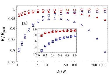
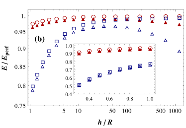
Figure 2: Ratio of numerically computed energies $E$ for realistic metals and $E_{\rm perf}$ for perfect metal against $h/R$. (a) two identical cylinders, (b) a cylinder and a plate. The parameters for the plasma model are $\lambda_{p}/R=0.05$, $0.5$ (open circles and open squares respetively). For the Drude model the same values of $\lambda_{p}/R$ are used; $\lambda_{p}/R=0.05$, $0.5$(filled and open triangles, respectively) and $\lambda_{p}/\lambda_{\sigma}=27.4$. Insets: Short distance range.

In Fig. 2, we show our numerical results for two parallel cylinders and also for a cylinder parallel to a plate. The graphs show the Casimir energies for the Drude and plasma cylinders, normalized to the energies of perfect metal cylinders. For the numerics we used $\lambda_{\rm p}/R=0.05$ and $0.5$ with $\lambda_{\rm p}/\lambda_{\sigma}=27.4$, corresponding to gold for which $\lambda_{\rm p}=137$ nm and $\lambda_{\sigma}\approx 5$ nm. Figure 2 clearly shows the material dependence of the Casimir energies. At large separations, for the plasma model, the ratios of $E/E_{perf}$ approach one. This is due to the fact that $\lambda_{\rm p}/R<1$ and we are in the universal regime, see Fig. 1. For Drude cylinders, the quantity $\xi^{\prime}$ determines the behavior of the curves. At $\lambda_{\rm p}/R=0.5$, one has $\ 5\times 10^{-4}<\xi^{\prime}<0.06$ and for $\lambda_{\rm p}/R=0.05$, $5\times 10^{-5}<\xi^{\prime}<0.006$ for the range of $h$ shown in Fig. (2). Since $\xi^{\prime}\ll 1$, we expect from our asymptotic computations that the Casimir energy is close to the energy for perfect metal cylinders. Fig. 2 indeed shows a plateau at intermediate distances that is approaching the perfect metal energy $E_{perf}$. This approach is better for $\lambda_{\rm p}/R=0.05$ which corresponds to a smaller $\xi^{\prime}$. At small distances, none of our asymptotic results applies and the actual energy is more strongly redruced compared to $E_{perf}$. With increasing distance, we expect at $\xi^{\prime}\sim 1$ a crossover to the non-universal asymptotic energy of Eq. (20). While this crossover is not fully shown in Fig. 2, the descrease of the energy ratio $E/E_{perf}$ with increasing separation is a precursor of this crossover. The same arguments apply to the interaction of a Drude cylinder with a plate.

We now compare our numerics with the PFA results at short separations and with the asymptotic results at large separations for both the plasma and the Drude models.

IV.1 PFA versus numerics

The PFA energy is obtained by integrating the PFA force $F=2\pi RE_{\rm plates}(h)$ with respect to $h$, where $E_{\rm plates}(h)$ is the energy of two parallel plates at distance $h$ given by the Lifshitz formula Lifshitz (1956) using the dielectric function of Eq. (2). Fig. 3 shows the numerically computed Casimir energy for $\lambda_{\rm p}/R=0.5$ and $0.05$, normalized to the PFA energy for parallel cylinders and a cylinder parallel to a plate. We find similar results for the Drude model. The energies associated with the Drude model are not shown here since they collapse on the data for the plasma model at short separations. Our data support the consistency of the PFA in the limit of vanishing separations.

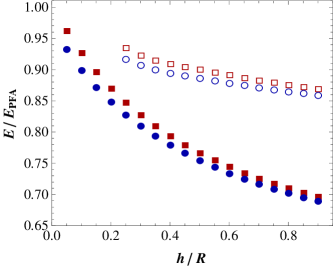
Figure 3: Ratio of the numerical results for the Casimir energy shown in Fig. 2 and the PFA energy based on the Lifshitz theory for the plasma model with $\lambda_{p}/R=0.05$ (squares) and $\lambda_{p}/R=0.5$ (circles). The ratio is shown as a function of the surface-to-surface distance $h$. Filled and empty shapes representing the data for parallel cylinders and cylinder–plate, respectively.

IV.2 Asymptotics versus numerics

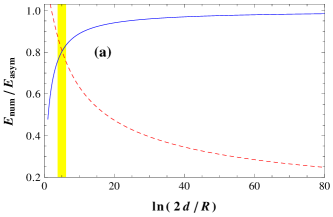
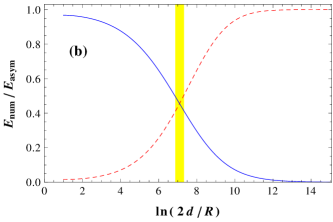
Figure 4: Two identical cylinders: Ratio of the numerically computed energy for the plasma model (a) and the Drude model (b) and the corresponding universal (blue solid line) and non-universal (red dashed line) asymptotic results with $\lambda_{\rm p}/R=5$ and $\lambda_{\sigma}=\lambda_{\rm p}/27.4$. The universal asymptotic energy is given by Eq. (14) and non-universal ones are given by Eqs. (17) and (20). The yellow strip shows the crossover region between the Drude and plasma asymptotic energies.

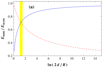
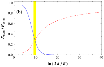
Figure 5: Same as Fig. 4 but for a cylinder and a plate with the universal asymptotic energy given by Eq. (25) and non-universal ones by Eqs. (27) and (28).

Figures 4 and 5 show the ratio of the computed energies and the corresponding asymptotic results (universal and non-universal regimes) versus $\ln(2d/R)$ for two cylinders and a cylinder parallel to a plate, respectively. The parameter that couples shape (radius) and material properties is chosen as $\lambda_{\rm p}/R=5$. Figures 4(a) and 5(a) show that for plasma cylinders, at intermediate separations, the energy normalized to the non-universal asymptotic energy is approaching unity whereas at asymptotically large separations the energy normalized to the universal asymptotic energy is tending to unity. On the other hand, Figs. 4(b) and 5(b) show that for Drude cylinders, at intermediate separations, the energy normalized to the universal energy is approaching unity whereas at asymptotically large separations the energy normalized to the non-universal energy is tending to unity. These figures confirm the validity of the crossover regime shown in Fig. 1.

V Summary

In summary, we have calculated the Casimir force between two metallic cylinders and a metallic cylinder parallel to a plate. The energy is calculated numerically for a large range of separations. We also find asymptotic energies for large separations and confirmed their validity with the numerical results. Furthermore, we showed that the numerics tend to the PFA energies at short separations.

The interesting phenomenon in our results is that the Casimir interaction involving Drude cylinders approaches a universal form of interaction at intermediate separations and becomes non-universal (material dependent) at larger distances $d\gtrsim R^{2}/\lambda_{\sigma}$. This behavior can be explained in terms of the size of the collective charge fluctuations in a Drude metal. However if $\lambda_{\rm p}\ll R$ then plasma oscillations are supported by the cylinders and at asymptotically large separations the interaction energy does show universality.

Based on recent experiments, the interactions between metals might not be consistent with the Drude model Decca et al. (2007). The asymptotic energies that we found in this work can be used to provide a clearer distinction between the Drude and plasma model predictions as compared to two plates or a plate and sphere Zandi et al. (2010). An estimate of the interaction between two gold cylinders with $R=10$nm, length $L=100\mu$m, $\lambda_{p}=137$nm and $\lambda_{\sigma}=5$nm at a distance $d=200$nm yields a force of $\approx 1$pN within the plasma description and $\approx 27$pN within the Drude model. These forces are in the experimentally detectable regime.

The significant feature of the interaction between a Drude cylinder with another Drude cylinder or a plate is that upon increasing the separation, the interaction can move from a universal regime to a non-universal one. This behavior can be understood from the wave equation for the electric field inside a Drude cylinder. For imaginary frequencies $\omega=ic\kappa$, the Helmholtz operator $\nabla^{2}+\epsilon(\omega)(\omega/c)^{2}$ for a good Drude conductor becomes $\nabla^{2}-8\pi^{2}\kappa/\lambda_{\sigma}$. We are interested in the maximal wave length of the field and hence charge fluctuations for a given $\kappa$. With the smallest transverse wave vector $k_{x}$, $k_{y}\sim 2\pi/R$ we find the dispersion relation

$$|k_{z}|\sim R^{-1}\sqrt{\kappa/\kappa_{c}-1}\,,\quad\kappa_{c}=\lambda_{\sigma}/R^{2}\,.$$ (29)

Hence, collective charge fluctuations on arbitrarily large scales exist only for $\kappa>\kappa_{c}$ which is a consequence of dimensionality that does not appear in the absence of transverse constraints ($R\to\infty$). For $\kappa<\kappa_{c}$ charge fluctuations break up into clusters of typical size $\sim R/\sqrt{1-\kappa/\kappa_{c}}$ due to finite conductivity. The spectral contribution to the interaction between cylinders at distance $d$ is peaked around $\kappa\sim 1/d$. If $d\lesssim 1/\kappa_{c}$ ($d/R\lesssim\sqrt{d/\lambda_{\sigma}}$, see Fig. 1(b)), collective charge fluctuations contribute strongly to the interaction and render it universal similar to perfect metal cylinders for which $\kappa_{c}\sim 1/\sigma\to 0$. In the asymptotic regime with $d\gtrsim 1/\kappa_{c}$ ($d/R\gtrsim\sqrt{d/\lambda_{\sigma}}$, see Fig. 1(b)), finite conductivity prevents fluctuations on arbitrarily large scales and hence the interaction is proportional to $\sigma$, i.e., non-universal. It is important to note that as $R$ goes to zero, $\kappa_{c}$ becomes larger, and in consequence the finite conductivity of the cylinder becomes more important.

Appendix A T-matrices

A.1 T-matrix of a cylinder

In this subsection, we derive the T-matrix of a dielectric cylinder that is placed in the vacuum. For this purpose, in part (A.1.1) we find a solution to the vector wave equation in terms of vector cylindrical harmonics. In part (A.1.2) we expand the electromagnetic field inside and outside of a cylinder in the basis of the solutions presented in the previous part. Then we find the expansion coefficients, which are the T-matrix elements, for the fields inside and outside the cylinder by matching the boundary conditions at the cylinder surface. Finally in part (A.1.3) we show that the derived T-matrix in the limit of perfect conductivity ($\epsilon\to\infty$) agrees with the T-matrix of a perfectly conducting cylinder.

A.1.1 Vector cylindrical harmonics

Vector cylindrical harmonics provide a basis in which divergence-less solutions of the vector Helmholtz equation can be expanded. As in the spherical case, the vector harmonics can be obtained by applying the curl operator to a vector field $\Phi_{k_{z}n}(\kappa,{{\bf x}})$ that is given in terms of the scalar harmonics. In the cylindrical case, however, this construction is simpler than in the spherical case since the vector field $\Phi_{k_{z}n}(\kappa,{{\bf x}})$ can be chosen to be parallel to the $z$-axis and hence does not change direction as it does in the spherical case where $\Phi_{lm}(\kappa,{{\bf x}})\sim{\bf x}$. Depending on the polarization we defined the two sets of regular cylindrical harmonics

$$\mathbf{M}^{\rm reg}_{k_{z}n}(\kappa,{\bf x}) = \frac{1}{\sqrt{k_{z}^{2}+\kappa^{2}}}\nabla\times\Phi^{\rm reg}_{k_{z}n}(\kappa,{\bf x})\,,$$ (30)

$$\mathbf{N}^{\rm reg}_{k_{z}n}(\kappa,{\bf x}) = \frac{1}{\kappa\sqrt{k_{z}^{2}+\kappa^{2}}}\nabla\times\nabla\times\Phi^{\rm reg}_{k_{z}n}(\kappa,{\bf x})\,,$$ (31)

for magnetic multipoles (TE waves) and electric multipoles (TM waves), respectively, with $p=\sqrt{k_{z}^{2}+\kappa^{2}}$ and the vector field

$$\Phi^{\rm reg}_{k_{z}n}(\kappa,{\bf x})=\hat{\mathbf{z}}\,I_{n}(\rho p)e^{in\theta}e^{ik_{z}z}\,,$$ (32)

where $\rho$, $\theta$ and $z$ are the cylindrical coordinates of ${\bf x}$. The analog basis $\mathbf{M}^{\rm out}_{k_{z}n}(\kappa,{\bf x})$, $\mathbf{N}^{\rm out}_{k_{z}n}(\kappa,{\bf x})$ for outgoing waves is obtained by replacing $I_{n}$ by $K_{n}$. These are transverse waves, i.e., $\nabla\mathbf{M}^{x}_{k_{z}n}=\nabla\mathbf{N}^{x}_{k_{z}n}=0$. They obey the relations $\mathbf{M}^{x}_{k_{z}n}=\frac{1}{i\kappa}\nabla\times\mathbf{N}^{x}_{k_{z}n}$, $\mathbf{N}^{x}_{k_{z}n}=\frac{1}{i\kappa}\nabla\times\mathbf{M}^{x}_{k_{z}n}$. In explicit form, they read

$$\mathbf{M}^{\rm reg}_{k_{z}n}(\kappa,{\bf x})=\left[\frac{in}{p\rho}I_{n}(p\rho)\,\hat{\bf\rho}-I^{\prime}_{n}(p\rho)\hat{\bf\theta}\right]e^{in\theta}e^{ik_{z}z}\,,$$ (33)

$$\mathbf{N}^{\rm reg}_{k_{z}n}(\kappa,{\bf x})=\frac{1}{\kappa}\left[ik_{z}I^{\prime}_{n}(p\rho)\,\hat{\bf\rho}-\frac{nk_{z}}{p\rho}I_{n}(p\rho)\,\hat{\bf\theta}\right.$$

$$\hskip 85.35826pt\left.-pI_{n}(p\rho)\hat{\mathbf{z}}\phantom{\frac{1}{\kappa}}\right]e^{in\theta}e^{ik_{z}z}\,.$$ (34)

It is analogous for the outgoing waves.

A.1.2 Scattering amplitudes

We consider an infinitely long dielectric cylinder with $\epsilon(ic\kappa)$, $\mu(ic\kappa)$ and radius $R$ in vacuum. We expand the electromagnetic field inside and outside the cylinder in the bases of Eqs. (30), (31) and the corresponding bases for outgoing waves. The expansion coefficients for the field inside and outside (T-matrix elements) follow from the matching conditions at the cylinder surface for the field components that are parallel to the surface.

For an incident magnetic multipole (TE) field, we make the scattering ansatz for the electric field modes

$$\mathbf{E}_{k_{z}n}^{M}(\kappa,{\bf x})=\mathbf{M}^{\rm reg}_{k_{z}n}(\kappa,{\bf x})+T^{MM}_{k_{z}n}\mathbf{M}^{\rm out}_{k_{z}n}(\kappa,{\bf x})\\ +T^{ME}_{k_{z}n}\mathbf{N}^{\rm out}_{k_{z}n}(\kappa,{\bf x})\,,$$ (35)

outside the cylinder and

$$\mathbf{E}_{k_{z}n}^{M}(\kappa,{\bf x})=A^{MM}_{k_{z}n}\tilde{\mathbf{M}}^{\rm reg}_{k_{z}n}(\kappa,{\bf x})+A^{ME}_{k_{z}n}\tilde{\mathbf{N}}^{\rm reg}_{k_{z}n}(\kappa,{\bf x})\,,$$ (36)

inside the cylinder where $\tilde{\mathbf{M}}^{\rm reg}_{k_{z}n}(\kappa,{\bf x})$, $\tilde{\mathbf{N}}^{\rm reg}_{k_{z}n}(\kappa,{\bf x})$ are given by Eqs.. (30), (31) with $\kappa$ replaced by $\kappa\sqrt{\epsilon(ic\kappa)\mu(ic\kappa)}$. For an incident electric multipole (TM) field, the ansatz becomes

$$\mathbf{E}_{k_{z}n}^{E}(\kappa,{\bf x})=\mathbf{N}^{\rm reg}_{k_{z}n}(\kappa,{\bf x})+T^{EM}_{k_{z}n}\mathbf{M}^{\rm out}_{k_{z}n}(\kappa,{\bf x})\\ +T^{EE}_{k_{z}n}\mathbf{N}^{\rm out}_{k_{z}n}(\kappa,{\bf x})\,,$$ (37)

outside the cylinder and

$$\mathbf{E}_{k_{z}m}^{E}({\bf x})=A^{EM}_{k_{z}m}\tilde{\mathbf{M}}^{\rm reg}_{k_{z}m}(\kappa,{\bf x})+A^{EE}_{k_{z}m}\tilde{\mathbf{N}}^{\rm reg}_{k_{z}m}(\kappa,{\bf x})\,,$$ (38)

inside the cylinder.

The continuity conditions require that the tangential fields $E_{z}$, $E_{\phi}$, $H_{z}=B_{z}/\mu$ and $H_{\phi}=B_{\phi}/\mu$ are continuous across the cylinder surface. Using the explicit expressions of Eqs. (33), (A.1.1) these conditions lead for each type of multipole fields to a set of four linear equations for the expansion coefficients. Using $\mathbf{B}=-(1/\kappa)\nabla\times\mathbf{E}$ and setting $p^{\prime}=\sqrt{\epsilon\mu\kappa^{2}+k_{z}^{2}}$ these equations can be written for incident magnetic (TE) waves as

$$M_{k_{z}n}\begin{pmatrix}A^{MM}_{k_{z}n}\\ T^{MM}_{k_{z}n}\\ A^{ME}_{k_{z}n}\\ T^{ME}_{k_{z}n}\end{pmatrix}=\begin{pmatrix}\frac{p}{\kappa}I_{n}(pR)\\ I^{\prime}_{n}(pR)\\ 0\\ \frac{nk_{z}}{pR\kappa}I_{n}(pR)\end{pmatrix}\,,$$ (39)

with the matrix

$$M_{k_{z}n}=\begin{pmatrix}\frac{p^{\prime}}{\mu\kappa}I_{n}(p^{\prime}R)&-\frac{p}{\kappa}K_{n}(pR)&0&0\\ I^{\prime}_{n}(p^{\prime}R)&-K^{\prime}_{n}(pR)&\frac{nk_{z}}{p^{\prime}\sqrt{\epsilon\mu}R\kappa}I_{n}(p^{\prime}R)&-\frac{nk_{z}}{pR\kappa}K_{n}(pR)\\ 0&0&\frac{p^{\prime}}{\sqrt{\epsilon\mu}\kappa}I_{n}(p^{\prime}R)&-\frac{p}{\kappa}K_{n}(pR)\\ \frac{nk_{z}}{\mu p^{\prime}R\kappa}I_{n}(p^{\prime}R)&-\frac{nk_{z}}{pR\kappa}K_{n}(pR)&\sqrt{\epsilon/\mu}I^{\prime}_{n}(p^{\prime}R)&-K^{\prime}_{n}(pR)\\ \end{pmatrix}\,,$$ (40)

For incident electric (TM) waves the linear equations are

$$M_{k_{z}n}\begin{pmatrix}A^{EM}_{k_{z}n}\\ T^{EM}_{k_{z}n}\\ A^{EE}_{k_{z}n}\\ T^{EE}_{k_{z}n}\end{pmatrix}=\begin{pmatrix}0\\ \frac{nk_{z}}{pR\kappa}I_{n}(pR)\\ \frac{p}{\kappa}I_{n}(pR)\\ I^{\prime}_{n}(pR)\\ \end{pmatrix}\,,$$ (41)

with the same matrix $M_{k_{z}n}$ as before. The solution to these equations for the T-matrix elements can be expressed as

$$T^{MM}_{k_{z}n}=-\frac{I_{n}(pR)}{K_{n}(pR)}\frac{\Delta_{1}\Delta_{4}+K^{2}}{\Delta_{1}\Delta_{2}+K^{2}}\,,$$ (42)

$$T^{EE}_{k_{z}n}=-\frac{I_{n}(pR)}{K_{n}(pR)}\frac{\Delta_{2}\Delta_{3}+K^{2}}{\Delta_{1}\Delta_{2}+K^{2}}\,,$$ (43)

$$T^{ME}_{k_{z}n}=-T^{EM}_{k_{z}n}=\frac{K}{\sqrt{\epsilon\mu}(pR)^{2}K_{n}(pR)^{2}}\frac{1}{\Delta_{1}\Delta_{2}+K^{2}}\,,$$ (44)

with

$$K=\frac{nk_{z}}{\sqrt{\epsilon\mu}R^{2}\kappa}\left(\frac{1}{p^{\prime 2}}-\frac{1}{p^{2}}\right)\,,$$ (45)

and

$$\Delta_{1} = \frac{I^{\prime}_{n}(p^{\prime}R)}{p^{\prime}RI_{n}(p^{\prime}R)}-\frac{1}{\epsilon}\frac{K^{\prime}_{m}(pR)}{pRK_{m}(pR)}\,,$$ (46)

$$\Delta_{2} = \frac{I^{\prime}_{n}(p^{\prime}R)}{p^{\prime}RI_{n}(p^{\prime}R)}-\frac{1}{\mu}\frac{K^{\prime}_{n}(pR)}{pRK_{n}(pR)}\,,$$ (47)

$$\Delta_{3} = \frac{I^{\prime}_{n}(p^{\prime}R)}{p^{\prime}RI_{n}(p^{\prime}R)}-\frac{1}{\epsilon}\frac{I^{\prime}_{n}(pR)}{pRI_{n}(pR)}\,,$$ (48)

$$\Delta_{4} = \frac{I^{\prime}_{n}(p^{\prime}R)}{p^{\prime}RI_{n}(p^{\prime}R)}-\frac{1}{\mu}\frac{I^{\prime}_{n}(pR)}{pRI_{n}(pR)}\,.$$ (49)

Notice that in general the polarization is not conserved under scattering, i.e., $T^{EM}_{k_{z}n}\neq 0\neq T^{ME}_{k_{z}n}$.

A.1.3 Limit of perfect conductivity

We consider the limit $\epsilon\to\infty$ with $\mu$ fixed. Then $p^{\prime}\to\sqrt{\epsilon\mu}\,\kappa$ and $K\sim 1/\sqrt{\epsilon\mu}$. In addition, we have for large $p^{\prime}$

$$\frac{I^{\prime}_{n}(p^{\prime}R)}{p^{\prime}RI_{n}(p^{\prime}R)}\to\frac{1}{p^{\prime}R}\to\frac{1}{\sqrt{\epsilon\mu}R\kappa}\,,$$ (50)

so that

$$\Delta_{1},\,\Delta_{3} \to \frac{1}{\sqrt{\epsilon\mu}R\kappa}+{\cal O}(\epsilon^{-1})\,,$$ (51)

$$\Delta_{2} \to -\frac{1}{\mu}\frac{K^{\prime}_{n}(pR)}{pRK_{n}(pR)}+{\cal O}(\epsilon^{-1/2})\,,$$ (52)

$$\Delta_{4} \to -\frac{1}{\mu}\frac{I^{\prime}_{n}(pR)}{pRI_{n}(pR)}+{\cal O}(\epsilon^{-1/2})\,.$$ (53)

This asymptotic forms show that the T-matrix elements that couple TM and TE waves vanish as

$$T^{ME}_{k_{z}n}\sim\frac{1}{\sqrt{\epsilon}}\to 0\,,$$ (54)

in the limit $\epsilon\to\infty$. The T-matrix elements that couple like polarizations simplify substantially. Since for $\epsilon\to\infty$

$$\frac{\Delta_{1}\Delta_{4}-K^{2}}{\Delta_{1}\Delta_{2}-K^{2}} \to \frac{I_{n}^{\prime}(pR)K_{n}(pR)}{I_{n}(pR)K^{\prime}_{n}(pR)}\,,$$ (55)

$$\frac{\Delta_{2}\Delta_{3}-K^{2}}{\Delta_{1}\Delta_{2}-K^{2}} \to 1\,,$$ (56)

we get the simplified expressions

$$T^{MM}_{k_{z}n} = -\frac{I_{n}^{\prime}(pR)}{K^{\prime}_{n}(pR)}\,,$$ (57)

$$T^{EE}_{k_{z}n} = -\frac{I_{n}(pR)}{K_{n}(pR)}\,,$$ (58)

$$T^{EM}_{k_{z}n} = T^{ME}_{k_{z}n}=0\,.$$ (59)

It is easily checked that these are the T-matrix elements for a scalar field with Neumann boundary conditions (magnetic or TE modes) and with Dirichlet boundary conditions (electric or TM modes). Hence, in the limit of perfect conductivity the EM scattering problem for a cylinder separates into two independent scalar problems, one with Dirichlet and one with Neumann boundary conditions.

A.2 T-matrix of a plate

The T-matrix elements of a plane is given by its Frensel coefficients Rahi et al. (2009)

$$T^{P}_{{\bf k}_{\bot}}=r^{P}(ic\kappa,(1+{\bf k}_{\bot}^{2}/\kappa^{2})^{-1/2})\,,$$ (60)

with $P$ the polarization index, ${\bf k}_{\bot}$ the momentum perpendicular to the $\hat{\bf x}$ direction, and $r^{Q}$ the Frensel coefficients

$$r^{M}(ic\kappa,x) =\frac{\mu(ic\kappa)-\sqrt{1+(n^{2}(ic\kappa)-1)x^{2}}}{\mu(ic\kappa)+\sqrt{1+(n^{2}(ic\kappa)-1)x^{2}}}\,,$$ (61)

$$r^{E}(ic\kappa,x) =\frac{\epsilon(ic\kappa)-\sqrt{1+(n^{2}(ic\kappa)-1)x^{2}}}{\epsilon(ic\kappa)+\sqrt{1+(n^{2}(ic\kappa)-1)x^{2}}},$$ (62)

here $\epsilon$, $\mu$ and $n(ic\kappa)$ are the dielectric response function, magnetic permeability, and the refractive index of the plate, respectively. The refractive index in terms of the dielectric function and the magnetic permeability of the plate is given by

$$n(ic\kappa)=\sqrt{\epsilon(ic\kappa)\mu(ic\kappa)}\,.$$ (63)

The T-matrix of a dielectric plate Eq. (60) is diagonal with respect to the polarization indices.

Appendix B Translation matrix

According to Graf’s addition theorem, the following relation holds,

$$K_{m}(p\,r_{j})\,e^{im\phi_{j}}=\\ \sum_{n=-\infty}^{\infty}(-1)^{n}K_{m-n}(p\,R_{ji})\,e^{-i(m-n)\,\phi_{ji}}I_{m}(p\,r_{i})\,e^{in\phi_{i}}\,,$$ (64)

where $\mathbf{r}_{j}=\mathbf{r}_{i}+\mathbf{R}_{ji}$ with $\mathbf{r}_{i}=r_{i}(\cos\phi_{i},\sin\phi_{i})$, $\mathbf{R}_{ji}=R_{ji}(\cos\phi_{ji},\sin\phi_{ji})$ are two-dimensional vectors in the $xy$-plane. We consider translations in 3D that are perpendicular to the $z$-axis with the translation vector $\mathbf{X}_{ji}=(\mathbf{R}_{ji},0)$, i.e., we set ${\bf x}_{i}=(\mathbf{r}_{i},z_{i})$ with $z_{i}=z_{j}$. Since the curl operator commutes with translations, from the definitions in Eqs. (30), (31) and the addition theorem of Eq. (64) follow the translation formulas from outgoing to regular waves

$$\mathbf{M}^{\rm out}_{k_{z}m}({\bf x}_{j}) = \sum_{n=-\infty}^{\infty}{{\mathcal{U}}}^{ij}_{k_{z}nm}\,\mathbf{M}^{\rm reg}_{k_{z}n}({\bf x}_{i})$$ (65)

$$\mathbf{N}^{\rm out}_{k_{z}m}({\bf x}_{j}) = \sum_{n=-\infty}^{\infty}{{\mathcal{U}}}^{ij}_{k_{z}nm}\,\mathbf{N}^{\rm reg}_{k_{z}n}({\bf x}_{i})$$ (66)

with the translation matrix

$${\mathcal{U}}^{ij}_{k_{z}nm}=K_{m-n}(p|\mathbf{X}_{ji}|)e^{-i(m-n)\phi_{ji}}\,.$$ (67)

From this we make two important observations: Translations conserve the polarization, i.e., they do not couple magnetic and electric modes, and the translation matrices are diagonal in $k_{z}$. The conservation of polarization leads to a diagonal translation matrix that acts on the full set of electric and magnetic modes.

Appendix C Conversion matrix from vector plane wave basis to cylindrical vector wave basis

In this section we show the conversion matrix elements from Ref. Rahi et al. (2009). The cylindrical vector wave functions are given in Eq. (30) and (31), which decay along the $-\mathbf{\hat{z}}$. We consider regular vector plane wave functions that decay along the $-\mathbf{\hat{x}}$ axis

$${{\bf M}^{\text{reg}}}_{\mathbf{k}_{\perp}}(\kappa,\mathbf{x})=\\ \frac{1}{\sqrt{k_{y}^{2}+k_{z}^{2}}}\boldsymbol{\nabla}\times e^{\sqrt{\kappa^{2}+k_{y}^{2}+k_{z}^{2}}x+ik_{y}y+ik_{z}z}\mathbf{\hat{x}},$$ (68)

$${{\bf N}^{\text{reg}}}_{\mathbf{k}_{\perp}}(\kappa,\mathbf{x})=\\ \frac{1}{\kappa\sqrt{k_{y}^{2}+k_{z}^{2}}}\boldsymbol{\nabla}\times\boldsymbol{\nabla}\times e^{\sqrt{\kappa^{2}+k_{y}^{2}+k_{z}^{2}}x+ik_{y}y+ik_{z}z}\mathbf{\hat{x}}.$$ (69)

The vector plane wave functions can be written in terms of vector cylindrical wave functions,

$${{\bf M}^{\text{reg}}}_{\mathbf{k}_{\perp}}(\kappa,\mathbf{x})=\sum_{n}D_{k_{z}nM,\mathbf{k}_{\perp}M}{{\bf M}^{\text{reg}}}_{k_{z}n}(\kappa,\mathbf{x})$$

$$+D_{k_{z}nE,\mathbf{k}_{\perp}M}{{\bf N}^{\text{reg}}}_{k_{z}n}(\kappa,\mathbf{x})\,,$$ (70)

$${{\bf N}^{\text{reg}}}_{\mathbf{k}_{\perp}}(\kappa,\mathbf{x})=\sum_{n}D_{k_{z}nM,\mathbf{k}_{\perp}E}{{\bf M}^{\text{reg}}}_{k_{z}n}(\kappa,\mathbf{x})$$

$$+D_{k_{z}nE,\mathbf{k}_{\perp}E}{{\bf N}^{\text{reg}}}_{k_{z}n}(\kappa,\mathbf{x})\,,$$ (71)

using the conversion matrix elements

$$D_{k_{z}nM,\mathbf{k}_{\perp}M} =-i\frac{k_{z}}{\sqrt{k_{y}^{2}+k_{z}^{2}}}\sqrt{1+\xi^{2}}\left(\sqrt{1+\xi^{2}}+\xi\right)^{n}\,,$$ (72)

$$D_{k_{z}nE,\mathbf{k}_{\perp}M} =i\frac{\kappa}{\sqrt{k_{y}^{2}+k_{z}^{2}}}\xi\left(\sqrt{1+\xi^{2}}+\xi\right)^{n}\,,$$ (73)

$$D_{k_{z}nE,\mathbf{k}_{\perp}E} =D_{k_{z}nM,\mathbf{k}_{\perp}M}\,,$$ (74)

$$D_{k_{z}nM,\mathbf{k}_{\perp}E} =-D_{k_{z}nE,\mathbf{k}_{\perp}M},$$ (75)

where $\xi=\frac{k_{y}}{\sqrt{\kappa^{2}+k_{z}^{2}}}$ and $\mathbf{k}_{\perp}=(k_{y},k_{z})$.

References

• Brown-Hayes et al. (2005) M. Brown-Hayes, D. A. R. Dalvit, F. D. Mazzitelli, W. J. Kim,  and R. Onofrio, Phys. Rev. A, 72, 052102 (2005).
• Decca et al. (2010) R. S. Decca, E. Fischbach, G. L. Klimchitskaya, D. E. Krause, D. López,  and V. M. Mostepanenko, Phys. Rev. A, 82, 052515 (2010).
• Sazonova et al. (2004) V. Sazonova, Y. Yaish, H. Ustunel, D. Roundy, T. A. Arias,  and P. L. Mceuen, Nature (London), 431, 284 (2004).
• Serry et al. (1998) F. M. Serry, D. Walliser,  and G. J. Maclay, Journal of Applied Physics, 84, 2501 (1998), ISSN 0021-8979.
• Buks and Roukes (2001) E. Buks and M. L. Roukes, Phys. Rev. B, 63, 033402 (2001).
• Šiber et al. (2009) A. Šiber, R. F. Rajter, R. H. French, W. Y. Ching, V. A. Parsegian,  and R. Podgornik, Phys. Rev. B, 80, 165414 (2009).
• Elliott (1968) G. F. Elliott, Journal of Theoretical Biology, 21, 71 (1968), ISSN 0022-5193.
• Parsegian (1972) V. A. Parsegian, J. Chem. Phys., 56 (1972), ISSN 0021-9606, doi:10.1063/1.1677878.
• Emig et al. (2006) T. Emig, R. L. Jaffe, M. Kardar,  and A. Scardicchio, Phys. Rev. Lett., 96, 080403 (2006).
• Rahi et al. (2008) S. J. Rahi, T. Emig, R. L. Jaffe,  and M. Kardar, Phys. Rev. A, 78, 012104 (2008).
• Rahi et al. (2009) S. J. Rahi, T. Emig, N. Graham, R. L. Jaffe,  and M. Kardar, Phys. Rev. D, 80, 085021 (2009).
• U. Mohideen and Mostepanenko (2009) M. B. U. Mohideen, G. L. Klimchitskaya and V. M. Mostepanenko, Advances in the Casimir Effect (Oxford University Press, 2009).
• Emig et al. (2009) T. Emig, N. Graham, R. L. Jaffe,  and M. Kardar, Phys. Rev. A, 79, 054901 (2009).
• Graham et al. (2010) N. Graham, A. Shpunt, T. Emig, S. J. Rahi, R. L. Jaffe,  and M. Kardar, Phys. Rev. D, 81, 061701 (2010).
• Maghrebi et al. (2011) M. F. Maghrebi, S. J. Rahi, T. Emig, N. Graham, R. L. Jaffe,  and M. Kardar, PNAS, 108, 6867 (2011).
• Zandi et al. (2010) R. Zandi, T. Emig,  and U. Mohideen, Phys. Rev. B, 81, 195423 (2010).
• Noruzifar et al. (2011) E. Noruzifar, T. Emig,  and R. Zandi, Phys. Rev. A, 84, 042501 (2011).
• Bordag et al. (2006) M. Bordag, B. Geyer, G. Klimchitskaya,  and V. Mostepanenko, Phys. Rev. B, 74, 205431 (2006).
• Bordag (2006) M. Bordag, Phys. Rev. D, 73, 125018 (2006).
• Lombardo et al. (2008) F. C. Lombardo, F. D. Mazzitelli,  and P. I. Villar, Phys. Rev. D, 78, 085009 (2008).
• Weber and Gies (2010) A. Weber and H. Gies, Phys. Rev. D, 82, 125019 (2010).
• Barash and Kyasov (1989) Y. Barash and A. Kyasov, Soviet Physics - JETP, 68, 39 (1989).
• Dobson et al. (2006) J. F. Dobson, A. White,  and A. Rubio, Phys. Rev. Lett., 96, 073201 (2006).
• Mazzitelli et al. (2006) F. D. Mazzitelli, D. A. R. Dalvit,  and F. C. Lombardo, New Journal of Physics, 8, 240 (2006).
• Drummond and Needs (2007) N. D. Drummond and R. J. Needs, Phys. Rev. Lett., 99, 166401 (2007).
• Dobson et al. (2009) J. F. Dobson, T. Gould,  and I. Klich, Phys. Rev. A, 80, 012506 (2009).
• Note (1) In the cylinder-plate case, we restricted the numerics to $h/R>0.3$ with $n_{\rm max}=41$ due to increasing numerical uncertainties in the $k_{y}$ integration in Eq. (7).
• Anderson et al. (1999) E. Anderson, Z. Bai, C. Bischof, S. Blackford, J. Demmel, J. Dongarra, J. Du Croz, A. Greenbaum, S. Hammarling, A. McKenney,  and D. Sorensen, LAPACK Users’ Guide, 3rd ed. (Society for Industrial and Applied Mathematics, Philadelphia, PA, 1999) ISBN 0-89871-447-8 (paperback).
• Lifshitz (1956) E. M. Lifshitz, Sov. Phys. JETP, 2, 73 (1956).
• Decca et al. (2007) R. S. Decca, D. López, E. Fischbach, G. L. Klimchitskaya, D. E. Krause,  and V. M. Mostepanenko, Phys. Rev. D, 75, 077101 (2007).