A morphological study of cluster dynamics between critical points

Abstract

We study the geometric properties of a system initially in equilibrium at a critical point that is suddenly quenched to another critical point and subsequently evolves towards the new equilibrium state. We focus on the bidimensional Ising model and we use numerical methods to characterize the morphological and statistical properties of spin and Fortuin-Kasteleyn clusters during the critical evolution. The analysis of the dynamics of an out of equilibrium interface is also performed. We show that the small scale properties, smaller than the target critical growing length $\xi(t)\simeq t^{1/z}$ with $z$ the dynamic exponent, are characterized by equilibrium at the working critical point, while the large scale properties, larger than the critical growing length, are those of the initial critical point. These features are similar to what was found for sub-critical quenches. We argue that quenches between critical points could be amenable to a more detailed analytical description.

1 Introduction

The relaxation dynamics of a macroscopic system taken to its critical point with some quenching protocol has received much attention. Most of the existing studies focused on the time evolution of global quantities (magnetization, susceptibility, correlation functions, etc.) and characterized their scaling properties with numerical simulations and renormalization group techniques [1, 2, 3, 4]. These studies are not restricted to any spatial nor order parameter dimensionality.

In two dimensional critical systems in equilibrium, powerful theoretical tools such as Coulomb gas methods [5], conformal field theory (CFT) [6] and stochastic Loewner evolution (SLE) [7, 8, 9], allowed one to characterize the geometric and statistical properties of a large variety of mesoscopic observables in great detail. These objects give a more complete image of the system’s equilibrium configurations than the global observables accessed with scaling arguments and renormalization group techniques. However, as far as we know, nothing is known about these objects during the out of equilibrium evolution of the same (and other) critical samples.

An extensive numerical and analytic investigation of the coarsening sub-critical dynamics of two dimensional models from a mesoscopic point of view was carried out in recent years. The models treated were the clean Ising model with non-conserved [10, 11, 12] and conserved [13] order parameter dynamics, the random ferromagnet with non-conserved order parameter dynamics [14] or still the $q$ state Potts model [15, 16]. These studies allowed one to build a rather complete picture of the geometric and statistical properties of the spin clusters in these bidimensional systems. More precisely, their domain and hull-enclosed areas as well as their boundary lengths and the relation between areas and perimeters were analyzed and characterized in detail.

The aim of this work it to present a similar study of relevant dynamic geometric objects during the critical non-equilibrium evolution of the $2d$ Ising model evolving from equilibrium at another critical point, in this case an infinite temperature configuration that is equivalent to critical uncorrelated site percolation. We use simple scaling arguments and extensive numerical simulations.

Let us be more specific about the objects of our study. The most natural objects to consider are the spin clusters, i.e. clusters of nearest neighbor spins on the lattice that point in the same direction. These clusters are accessible via direct observation of the system. However, at the critical point, they are not appropriate to describe the critical equilibrium properties of the Ising model since their shape and statistical properties are not only dictated by the physical correlations but also by purely geometrical factors [17, 18]. To remedy this problem one has to consider, in place, smaller clusters, namely the Fortuin-Kasteleyn (FK) ones, that capture exclusively the equilibrium physical correlations in the system. Although not relevant to describe the equilibrium physical macroscopic properties of the samples the spin clusters are, nonetheless, also critical at the phase transition. Consequently, they are characterized by a different set of exponents from the ones of the FK clusters. For this reason (to be explained more thoroughly in Sec. 2.2) spin clusters are also interesting to analyze and we study both types of clusters here.

The article is organized as follows. In Sec. 2 we list the definitions of the different objects we study. The concrete analysis is presented next. We first check that the dynamical exponent $z$ governing the critical dynamics of spin clusters is actually the one of the $2d$ Ising model, as obtained with other means, as the dynamic renormalization group method [2]. To the best of our knowledge, this has never been brought to light before. We then study in full extent the number densities of various quantities giving access to the structure of spin clusters on a large interval of sizes. The validity of the dynamical scaling hypothesis is tested upon these number densities. Relations between areas and boundaries are also explored. The same method is applied to the FK clusters. We later turn our attention to the dynamics of a single interface and the comparison with the equilibrium results given by conformal field theory and stochastic Loewner evolution. This is the content of Sec. 3. Finally, in Sec. 4 we draw our conclusions and we discuss some lines of future research.

2 Definitions

2.1 Spin and Fortuin-Kasteleyn clusters

Simple scaling arguments from percolation theory [19] suggest that, in equilibrium, the divergence of the mean size of some kind of finite cluster at the critical point should be governed by the susceptibility exponent or, equivalently, the one of the spin-spin correlation function, that is the same as the probability for two spins to be in the same such cluster. The ensemble of nearest-neighbor spins that are parallel to each other constitute a domain or spin cluster. These are the most natural geometric objects, the critical properties of which one would expect to be linked to the ones of macroscopic physical observables. However, spin clusters do not capture the underlying critical properties of statistical physics models. This fact was first noticed by Sykes and Gaunt [17] who remarked that the mean size of the finite domains of the Ising model on a two dimensional lattice (2dIM) diverges at the critical point with an exponent that is different from the magnetic susceptibility exponent (see Table 1). Moreover, at infinite temperature there are spin clusters of arbitrary large size although the spin-spin correlation function vanishes. Still, for the particular case of the 2dIM, domains are critical at the critical point although they do not give access to the relevant critical exponents of the model. We will come back to this point in Sec. 2.2. In three dimensions, this is not the case and these spin clusters do not even percolate at the critical point [20].

The point was then to build clusters containing just physical correlations between spins (and not trivial geometric ones). This is achieved by the Fortuin-Kasteleyn clusters [21], proposed by these authors as a way to describe with the random cluster model percolation, the Ising model, the Potts model and many other statistical models. Independently, Coniglio and Klein [18] linked the critical properties of the Ising model to the percolation of Ising droplets which were later identified with the Fortuin-Kasteleyn clusters, the name that prevailed in the literature. The Fortuin-Kasteleyn clusters are constructed as follows. Starting with a spin domain, one first draws all bonds linking nearest-neighbor spin on the cluster and then erases bonds with a temperature dependent probability $e^{-2K}$. In such a way, the original bond-cluster typically diminishes in size and may even get disconnected. More precisely, the construction of these clusters from the partition function ${\cal Z}$ is the following. One rewrites the exponential of the sum as a product of exponentials:

$${\cal Z}=\sum_{\{\sigma\}}e^{K\sum_{\langle i,j\rangle}\sigma_{i}\sigma_{j}}=\sum_{\{\sigma\}}\prod_{\langle i,j\rangle}e^{K\sigma_{i}\sigma_{j}},$$ (1)

with $K=J/(k_{B}T)=\beta J$, $J$ the exchange coupling and $k_{B}$ the Boltzmann constant. Hereafter we measure temperature $T$ in units of $J/k_{B}$. By remarking that, since $\sigma_{i}\in\{-1;1\}$,

$$e^{K\sigma_{i}\sigma_{j}}=e^{K}\ [(1-e^{-2K})\delta_{\sigma_{i},\sigma_{j}}+e^{-2K}],$$ (2)

${\cal Z}$ can be recast in the form:

$${\cal Z}=e^{mK}\sum_{\{\sigma\}}\prod_{\langle i,j\rangle}[p\delta_{\sigma_{i},\sigma_{j}}+(1-p)],$$ (3)

with $m$ the total number of bonds of the lattice ($m=3L^{2}$ for a planar triangular lattice of linear size $L$) and $p=1-e^{-2K}$. By expanding the product, if $\sigma_{i}=\sigma_{j}$ one keeps the bond $\langle i,j\rangle$ with probability $p$ or erases it with probability $1-p$. The broken bonds ($\sigma_{i}=-\sigma_{j}$) are never kept. A connected collection of kept bonds is a Fortuin-Kasteleyn (FK) cluster. This whole construction is called the Fortuin-Kasteleyn random cluster model and an example is presented in Fig. 1. These clusters possess the searched properties. Their exponents are those of the Ising model [22]. For example, the probability for two spins to belong to the same FK cluster is exactly the spin-spin correlation of the Ising model. Note that the FK construction can be easily extended to all $q$-state Potts models, even with non integer $q$, in any dimensions.

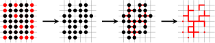
Figure 1: Sketch of the construction of a FK cluster. A domain is identified. The bonds between nearest-neighbor aligned spins (represented with black dots on the lattice sites) are erased using the FK procedure. Two FK disconnected clusters remain. The surviving bonds are highlighted on the edges of the lattice.

2.2 A few hints on conformal field theory

The existence of two types of critical clusters, the spin and FK ones belonging to distinct universality classes is valid for all $q$-state Potts model with $0\leq q\leq 4$ in two dimensions. In order to understand this point it is useful to consider the Coulomb gas formulation of the Potts model [5]. In this formulation, the $2d$ $q$-state Potts model can be described by the parameter $\kappa\in[4,8]$ such that

$$\sqrt{q}=-2\cos\left(\frac{4\pi}{\kappa}\right).$$ (4)

We choose a convention such that $\kappa$ also corresponds to the SLE parametrization for the interfaces associated to the $q$-state Potts model. We will come back to this point in Sec. 3.4 where we will study the behaviour of an out of equilibrium interface. The parameter $\kappa$ is also related to the central charge of the corresponding conformal field theory by the relation [5, 6]:

$$\mathrm{c}=\frac{1}{4}(6-\kappa)\left(6-\frac{16}{\kappa}\right).$$ (5)

For $\kappa\in[8/3,4]$ this Coulomb gas representation describes another class of models, the tricritical Potts model, i.e. Potts models with dilution. Note that the central charge is invariant under the transformation $\kappa\rightarrow 16/\kappa$ which maps a critical $q$-state Potts model onto a tricritical Potts model with a different number of states given by eq. (4). This means that there exist two critical theories for a given central charge. One is associated to the critical Potts model and the relevant structures are the FK clusters. The other one is the tricritical Potts model and the relevant clusters are the domains or spin clusters. This duality is such that the geometrical clusters of one model are the FK clusters of the other model and vice versa [23, 24].

The tricritical model associated to the $2d$ Ising model ($\kappa=16/3$) is the dilute $q=1$ Potts ($\kappa=3$). Both models possess the same central charge $\mathrm{c}=1/2$ but the same quantities in the two model are not associated to the same operators of the CFT. In $2d$ the spin clusters of the Ising model are the critical objects of the dilute $q=1$ Potts model [25]. This explains why the percolation exponents associated to the spin clusters are not related to the Ising model exponents but in fact are those of the tricritical $q=1$ Potts model, described by $\kappa=3$.

The critical exponents can then be expressed in term of $\kappa$. For instance, the fractal dimensions $D_{c}$, $D_{h}$ and $D_{ep}$ of the cluster area, its hull and its external perimeter (a precise definition of these quantities will be given in Sec. 2.3) read [26, 23]:

$$D_{c} = 1+\frac{3\kappa}{32}+\frac{2}{\kappa},$$ (6)

$$D_{h} = 1+\frac{\kappa}{8},$$ (7)

$$D_{ep} = 1+\frac{2}{\kappa}.$$ (8)

Note that the duality $\kappa\rightarrow 16/\kappa$ relates the fractal dimension of the external perimeter to the dimension of the hull of the dual model, such as $D_{ep}(\kappa)=D_{h}(16/\kappa)$ for $\kappa\geq 4$. This relation is called Duplantier duality [23]. For $\kappa<4$ the external perimeter coincides with the hull since they are no fjords. In this case the relation between $D_{ep}$ and $D_{h}$ mentioned above does not hold anymore and in fact $D_{ep}=D_{h}$.

	$\mathrm{c}$	$\kappa$	$q$	$D_{c}$	$D_{h}$	$D_{ep}$
percolation	0	6	1	91/48	7/4	4/3
Ising FK clusters	1/2	16/3	2	15/8	5/3	11/8
Ising spin clusters	1/2	3	1	187/96	11/8	11/8

Table 1: Central charge, $\mathrm{c}$, Coulomb gas or SLE parameter, $\kappa$, Potts model parameter, $q$ [all these related by eqs. (4) and (5)], and three fractal dimensions at the percolation threshold, and for FK and spin clusters at the critical point of the $2d$ Ising model. The c subscript in the fractal dimension is for the cluster mass, the h one for its hull, and ep for its external perimeter.

Finally, let us note that the existence of two types of critical clusters at the critical point is specific to the $2d$ Potts model. While the FK clusters can be defined for more general models, nothing ensures that they are critical at the transition point. For instance, FK clusters are not critical at the critical point in $2d$ parafermionic models [27]. Concerning the spin clusters, it is not even sure that they are critical at the critical point as in the $3d$ Ising model we have already mentioned.

2.3 Definitions of the quantities computed

In this section we define the quantities that we will consider in this work. We call a domain or spin cluster a connected set of sites with spins taking the same value. The mass (area in $2d$) of a domain is the number of sites belonging to it. A broken bond is a link of the lattice between two neighboring spins with different value (see Fig. 2).

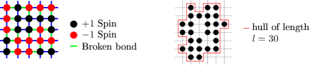
Figure 2: Left: sketch of an Ising spin configuration with the two-valued spins represented by black and red (black and grey) dots on the square lattice sites. Broken bonds are drawn with green (light grey) lines on the edges of the lattice. Right: a domain is singled out and its hull is represented with a thin red line.

The domain wall of a spin cluster is its external and internal contour, constructed as follows. One first generates a dual lattice by placing a site at the center of each plaquette of the original lattice. Next, the links on the dual lattice that cross broken bonds on the original lattice are joined together. In this way, one finds a closed loop on the dual lattice that runs along the internal or external boundary of a spin cluster in the way sketched in Fig. 2 for the external component. There is not much theoretical knowledge on this object and it is therefore more convenient to study other geometrical quantities which have received a theoretical description in equilibrium.

The hull of a cluster is restricted to the external part of the contour, that is to say, one excludes the contribution of the holes of the cluster (see Fig. 2). The hull enclosed area is the area, i.e. the total number of sites, inside the hull (the holes within the domains are thus filled). In the example in the right of Fig. 2 the hull-enclosed area is 29.

The length of the different types of contours defined above and living on the dual lattice is computed by counting the number of broken bonds corresponding to the object of concern that are crossed by the boundary. We can also define the external perimeter built by closing the narrow gates of the hull, making in this way a smoother version of the contour by eliminating the deep fjords. The meaning of narrow will be discussed later. As an example, on a square lattice, a cluster composed of a unique spin has a hull of length $4$ and an area equal to $1$ while for a two-spin cluster the hull length is $6$ and the area equals 2.

The FK clusters are defined on the edges of the lattice and not on the sites of the lattice as for the spin clusters. Therefore the length of their contour on the dual lattice is not proportional to the number of broken bonds. Indeed some bonds linking two sites of a FK cluster may not be within the cluster if they have not been kept in the construction of the cluster. In order to define the border of an FK cluster we then use a different sub-lattice, with four sites associated to an original one as shown in Fig. 3. The distance between two nearest-neighbor sub-sites counts as the unit of length for the contour. As an example, the cluster in Fig. 3 has a hull length of 24.

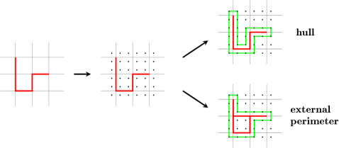
Figure 3: Left: an example of an FK cluster. Center: the sites of the sub-lattice associated to the original square lattice are added as small points. Right: the hull and the external perimeter of the chosen FK cluster are shown with a thin green line.

In Fig. 3 we also present the construction of the external perimeter of an FK cluster. To measure its length, the procedure is the following: all the bonds between nearest-neighbor sites (on the original lattice) belonging to the FK cluster are drawn, and then the walker is allowed to wander around this new cluster, that is to say, on the sites of the sub-lattice introduced before. The external perimeter is a smoother version of the hull and it has, consequently, a smaller fractal dimension. The cluster in Fig. 3 has an external perimeter of length 20 which is effectively smaller than its hull length.

2.4 Statistical and geometric properties in equilibrium

To describe the statistical and geometrical properties of the spin and FK clusters we used the tools of percolation theory (see e.g. [19]). For example, we counted the number of spin clusters with a given area for numerous samples and we thus obtained, after normalization, the number density of the spin cluster areas. We followed this procedure for the hull lengths, the hull-enclosed areas, etc. In general, when we consider the probability distribution per lattice site $n_{x}(X)$ (of a given geometrical object $x$ taking values $X$) which follows a power law, we denote the related critical exponent $\tau_{X}$, i.e.,

$$n_{x}(X)\sim X^{-\tau_{X}}.$$ (9)

Either the clusters or their boundaries are fractal objects at the critical point. Their Hausdorff dimension (referred hereafter as fractal dimension) is non-trivial and has been related to other critical exponents. Indeed, the fractal dimension $D_{X}$ of the objects described by the quantity $X$ can be expressed in terms of $\tau_{X}$:

$$D_{X}=\frac{d}{\tau_{X}-1},$$ (10)

with $d$ the dimensionality of the lattice [19]. A few examples are given in Table 1.

In finite-size lattices a cluster is said to percolate whenever it spans over a distance that is larger than the linear size $L$ of the system, in at least one direction of the lattice. The hull-enclosed areas do not exhibit a fractal structure since they have no holes. Their fractal dimension is therefore $2$. Their boundaries behave differently and they are fractal. Furthermore, Cardy and Ziff [28] showed that the number density of hull-enclosed areas behaves as:

$$n_{h}(A)\sim\frac{C}{A^{2}}$$ (11)

for $L^{2}\gg A^{2}\gg a^{2}$ with $C=1/(8\sqrt{3}\pi)$ at the percolation threshold and $C=1/(16\sqrt{3}\pi)$ for Ising spin clusters. The microscopic cut-off $a$ is the lattice spacing.

3 Critical dynamics

The stochastic relaxation dynamics after a quench to the critical point has been performed with a time dependent extension of the renormalization group method. Scaling laws for averaged global observable such as correlation functions and others have been obtained in many different systems. The growth of an equilibration length, $\xi(t)\leavevmode\nobreak\ \sim\leavevmode\nobreak\ t^{1/z}$ with $z$ the dynamic critical exponent, was evidenced. In this section we study the critical dynamics from a mesoscopic point of view and we show that this growing length also plays an important role in the characterization of the statistical properties of fluctuating quantities.

3.1 Description of the protocol

In this section we study the evolution of a system after a quench from $T=\infty$ to $T_{c}$. We first consider spin clusters on a triangular lattice for which $T_{c}=4/\ln 3$. The choice of a triangular lattice is motivated by the fact that the infinite temperature point exactly corresponds to a site percolation critical point on this lattice. Indeed, the site percolation threshold for this lattice is $p_{c}=1/2$ [29] so that, if we consider the number density of domains, the system is exactly at the percolation threshold at infinite temperature where the spins take the values $1$ or $-1$ with equal probability. For the quench considered, the system is initially in equilibrium at a critical state and after the quench it evolves towards equilibrium at another critical state, the one at $T_{c}$.

At infinite temperature FK clusters are not critical, actually they are trivial, for any lattice so it is immaterial to use the triangular or any other one. For this reason, in our study we used a square lattice. For the square lattice $T_{c}=2/\ln(1+\sqrt{2})$ and the infinite temperature point is not even a critical one for the spin clusters since here $p_{c}>1/2$. (Having said this, the studies in [10, 11, 12] showed that, somehow surprisingly, the sub-critical Monte Carlo dynamics of such a non-critical initial state gets, after a few time steps, very close to the critical percolation point as far as the properties of spin clusters are concerned. For instance, their number densities rapidly develop the critical percolation tails and only later the dynamics evolve towards the target equilibrium state at low temperature.)

The simulations were carried out on a lattice of linear size $L$ with periodic boundary conditions in both directions. For the initial condition at infinite temperature, the spins were chosen randomly with equal probability of being up or down. Once the system was prepared in the desired initial condition, single spin updates were performed at the temperature of the quench. A Monte Carlo time step (MCs) corresponds to $L^{2}$ single spin updates. The updates were accepted or rejected via the standard Monte Carlo Metropolis scheme. We gathered around $6\ 10^{5}$ independent samples. Unless stated otherwise, the lattice used has a linear size $L=1000$ for the analysis of spin clusters and $L=320$ for the study of FK clusters. For each sample we computed the desired quantities every $2^{n}$ MCs with $n\in[1,12]$.

For the spin clusters, the algorithm distinguishes first between the internal and external part (hull) of the perimeter and then calculates the length of the hulls, i.e. the number of broken external bonds. To do so the lattice is scanned and when a broken bond that has not been counted yet is found, the algorithm follows the boundary in a precise direction and keeps track (with a cumulative angle) of the path followed. Then, depending on the sign of the angle the boundary drawn is an external or an internal one. Some clusters (spanning ones) have a boundary with a vanishing angle. Those boundaries run across the system from one side to another so they are not homotopic to a point on the torus. We checked that these clusters are sufficiently rare so that we can discard them without affecting the statistics. For the FK clusters the process is the same on the sub-lattice evoked above. The algorithm walks on the sub-lattice around the FK clusters and once a contour is formed, the angle is measured to discriminate between internal and external contours and their lengths are computed.

The number densities obtained via this Monte Carlo method present a great dispersion, especially for large clusters which are much rarer than the small ones. This dispersion has been greatly suppressed by choosing appropriate bin sizes to construct the histograms, and to extract from them the distributions.

3.2 Spin clusters

We first briefly present the simulations performed to check whether the dynamical exponent governing the dynamics of the spin clusters conforms to the one extracted from the analysis of the correlation functions that is well documented in the literature [30, 31, 3]. Then we present the results for the spins clusters on a triangular lattice after the quench.

3.2.1 The dynamic exponent

As explained in Sec. 2.2, the critical geometric clusters of the $2d$IM are well understood as they are the FK clusters of the tricritical $q=1$ Potts model. However, it is not obvious whether this correspondence should hold in an out of equilibrium situation, typically a quench towards the critical point. In particular, one may wonder whether the dynamical exponent $z$ for spin clusters is the Ising one. To check this reasonable assumption, we calculated specific quantities that allow us to extract spin clusters exponents. For example, in equilibrium, the size of the largest spin cluster scales as $L^{-(\beta/\nu)_{tri}}$ where $(\beta/\nu)_{tri}=5/96$ and $\beta_{tri}$ is the magnetic exponent of the tricritical $q=1$ Potts model, $\nu_{tri}$ is the exponent associated to the divergence of the correlation length and $L$ is the linear size of the sample. We denote this quantity $M_{g}$. We now consider a quench from $T=0$ to $T_{c}$ for different system linear sizes $L$, and we compute $M_{g}(t)$. We consider this quench since the scaling form is simple in this case and the dynamical exponent should not depend upon the initial condition as long as we quench at the critical temperature. The inset of Fig. 4 shows the relaxation of this quantity for several sizes. We then apply the following scaling $M_{g}(t)\rightarrow M_{g}(t)L^{(\beta/\nu)_{tri}}$ and $t\rightarrow t/L^{z}$. The collapse of the different curves giving access to $z$ is presented in Fig. 4. The value obtained converges towards the most accurately estimated value $z=2.1667\ (5)$ [31]. This gives strong evidence that the dynamics of the spin clusters are indeed governed by the Ising dynamical exponent $z$. In consequence we will use the same $z$ for all the quantities computed in this work.

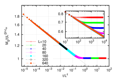
(a)

Figure 4: Geometrical cluster magnetization $M_{g}(t)$. The main part shows the collapse onto a master curve with the rescaling $t\to t/L^{z}$ and $M_{g}(t)\to M_{g}(t)L^{(\beta/\nu)_{tri}}$. In the inset we show the raw data $M_{g}(t)$ versus time for different system linear sizes $L$.

3.2.2 Hull-enclosed area number density

In Fig. 5 we present the distribution of the hull-enclosed areas, $n_{h}(A,t)$, at different times after the quench. In the first panel, Fig. 5(a), we display the distributions, $n_{h}$, versus the hull-enclosed area $A$. As expected from the results of Cardy and Ziff [28], the slopes of the initial and asymptotical (equilibrium at $T_{c}$) distributions equal $-2$ in a double logarithmic plot but the prefactors are slightly different. For this reason, the changes occurring in the distributions are very small. Equilibrium data (generated with a special purpose algorithm at $T_{c}$) are shown with (green at $T\to\infty$ and red at $T_{c}$) dashed lines. The bumps at large sizes correspond to the spanning clusters with a linear size of the order of $L$, the linear size of the system, are finite size effects. Note that the position of the bump and the very last part of the $n_{h}(A,t)$ close to it, are time-independent (within our numerical accuracy and for the times accessed in the simulation).

For hull-enclosed areas dynamic scaling suggests

$$n_{h}(A,t)\simeq A^{-\tau}\ g\left(\frac{A}{t^{\alpha}}\right)$$ (12)

for $A_{0}\ll A\ll L^{2}$ with $A_{0}=a^{2}$ a microscopic area scale and $L^{2}$ the macroscopic one. To make the notation lighter we did not add any sub-script to $\tau$ and $\alpha$. The exponents are given by

$$\tau=1+d/D,\qquad\qquad\alpha=D/z.$$ (13)

Since these areas are regular, i.e. they have no holes, $D=d=2$ and

$$\tau=2,\qquad\qquad\alpha=2/z.$$ (14)

Consistency with the asymptotic limit requires $g(y\to 0)=C$ and $g(y\to\infty)=2C$.

In order to test the dynamical scaling hypothesis, we impose the value $\tau=2$ and rescale the areas by a factor $t^{\alpha}$ with $\alpha$ a free parameter whose value is determined by the collapse of the numerical data on a master curve. The best collapse is obtained for $\alpha=0.92\ (5)$ and is seen in Fig. 5(b) with the theoretical percolation and Ising critical distributions being just horizontal after the given ordinate rescaling. The numerical equilibrium critical distributions (red dashed line for $T_{c}$ and green dashed line for $T\to\infty$) have been placed at convenience (horizontally) to ease the comparison with the other distributions. The horizontal dotted lines correspond to the exact prefactors $C=1/(16\sqrt{3}\pi)$ and $2C$ for the critical Ising and percolation distributions, respectively. The value of $\alpha$ is in agreement with the expected value $\alpha=2/z\simeq 0.92306$ with $z\simeq 2.1667\ (5)$ [31] since the hull-enclosed areas scale as the square of the dynamical length scale $\xi(t)\sim t^{1/z}$. It is quite remarkable that, while no time-dependent rescaling has been applied to the distribution, the curves collapse so accurately in the vertical direction. One may remark that the scaling is not so good for times that are smaller than 64 MCs, which is not surprising since the dynamical scaling hypothesis only holds after a non-universal time-scale.

In curvature-driven coarsening we know from [11, 13], that $n_{h}(A,t)=2C/(A+\lambda_{h}t)^{2}$ if we use an infinite temperature initial condition, i.e. $n_{h}(A,0)=2C/A^{2}$, with $\lambda_{h}$ a non-universal parameter. It implies

$$A^{\tau}n_{h}(A,t)=f(A/\lambda_{h}t)\quad\mbox{with}\quad f(x)=\frac{2C}{(1+1/x)^{2}}.$$ (15)

$f(x)$ looks like the right part of $A^{\tau}n_{h}(A,t)$ for $A>t^{2/z}$ in our case. Since we consider a situation with two critical points and not only one as in the sub-critical case we are tempted to think that the minimum of $g(x)$ around $x\simeq 1$ and more generally its non-monotonic behaviour can be

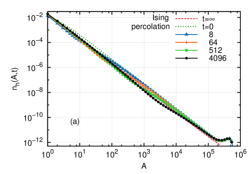
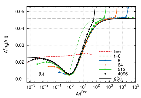
Figure 5: Spin clusters hull-enclosed area number densities in the $2d$IM on a triangular lattice are presented. (a) With dashed (red and green) lines equilibrium data at $T\to\infty$ and $T_{c}$. With solid lines the raw dynamic data for the times given in the key (in MCs) including the spanning clusters using a double logarithmic scale. (b) The areas in the x-axis are rescaled by the factor $t^{\alpha}$, with $\alpha=0.92$ consistently with the expectation $\alpha=D/z=2/z$. The distributions in the y-axis (in linear scale) are multiplied by $A^{\tau}=A^{2}$. The grey dotted horizontal lines at $0.046$ and $0.023$ are the theoretical predictions for the $T\to\infty$ critical site percolation point and the $T_{c}$ one, respectively, and $g(x)$ is the fitting function defined in eq. (12), and discussed in the text.

reproduced with a sum of two functions similar to $f(x)$, one decreasing from $C$ to $0$ and one increasing from $0$ to $2C$. This suggests for $g(x)$ defined in eq. (12) the form:

$$g(x)=C\left(\frac{1}{(1+ax^{b})^{c}}+\frac{2}{(1+(ax^{b})^{-1})^{c}}\right).$$ (16)

We left the powers $b$ and $c$ as free parameters as there is a priori no reason for them to be simple integers as in the sub-critical coarsening situation. Numerical inspection of the data shows a good fit for the values $a\simeq 0.65$, $b\simeq 0.79$ and $c\simeq 2.3$. Roughly speaking, $a$ fixes the position of the minimum, $b$ its width and $c$ its depth. Note that $c$ is chosen to allow the fitting curve $g(x)$ to go through the minimum of the numerical data but we do not attribute a special meaning to this value. Indeed the expansion of $g(x)$ close to the asymptotic values $C$ and $2C$ is proportional to $x^{b}$ and $x^{-b}$, respectively, both independant of $c$.

3.2.3 Hull-enclosed areas and hull lengths

As in [11, 13, 16] we study the relation between the hull-enclosed areas and the hull lengths by tracing an averaged scattered plot of $A$ against $p$ in Fig. 6. In panel (a) we show the raw data for different times after the critical quench. In panel (b) we scale the data by the relevant typical growing scales. In the case of the hull-enclosed areas this is the linear growing length, $\xi(t)$, to the power of their fractal dimension that is simply $D=d=2$ for these regular objects. In the case of the hull lengths, instead, the relevant linear scale is still the growing length, $\xi(t)$, now to the power of the hulls fractal dimension in the critical Ising point, which is $D^{I}_{h}=11/8$, as given in Table 1. The master curve shows a clear cross-over between two power law behaviors with the powers $D/D_{h}^{I}=16/11\simeq 1.45$ controlling the small scales and $D/D_{h}^{P}=8/7\simeq 1.14$ controlling the large scales. Summarizing,

$$\displaystyle{\left(\frac{A}{t^{D/z}}\right)\simeq\left(\frac{p}{t^{D_{h}^{I}/z}}\right)^{\zeta}\qquad\mbox{with}\qquad\zeta\ =\ \left\{\begin{array}[]{l}D/D_{h}^{I}\qquad\mbox{for}\qquad p/t^{D_{h}^{I}/z}\ll 1,\\ D/D_{h}^{P}\qquad\mbox{for}\qquad p/t^{D_{h}^{I}/z}\gg 1.\end{array}\right.}$$ (19)

3.2.4 Hull length number density

Next we proceed with the hull length distribution displayed in Fig. 7. In the first graph, Fig. 7(a), we show the distributions $n_{h}(p,t)$ vs. $p$ for various times after the quench where $p$ stands for the hull length. For this quantity, the equilibrium behavior for the critical Ising model is $n_{h}(p)\sim\leavevmode\nobreak\ p^{-27/11}$ and it is different from percolation criticality where $n_{h}(p)\sim\leavevmode\nobreak\ p^{-15/7}$. These equilibrium curves are drawn with dashed lines in the figure. We see in Fig. 7(a) that the dynamic curves interpolate between these two critical laws. For example, we can observe that for $t\leavevmode\nobreak\ =\leavevmode\nobreak\ 4096$ MCs there is a qualitative change for $p\leavevmode\nobreak\ \sim\leavevmode\nobreak\ 2000$. However, since the difference between $27/11$ and $15/7$ is small it is still difficult to get a precise picture of what is happening with this data representation. Note that, contrary to what happens with the area number densities, the time-dependence is seen in the full extent of the curves and not only for (relatively) small scales. Even the bump is displaced towards shorter lengths in the course of time.

A better description is given in Fig. 7(b) where we drew the same distribution multiplied by $p^{\tau}$ with $\tau={27/11}$, the exponent of the tail in the equilibrium distribution at $T_{c}$, so that the Ising equilibrium critical distribution is horizontal. As before, the lengths are rescaled by a factor $t^{\alpha}$ to take into account the growing length scale. Searching the value of $\alpha$ that gives the best horizontal collapse we find $\alpha=0.63\ (3)$. This fits well with the value expected from dynamical scaling argument such that $p$ is rescaled by $\xi(t)^{D_{h}}$ with $D_{h}=D^{I}_{h}=11/8=1.375$ the fractal

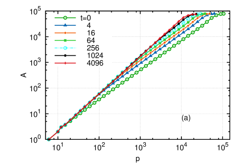
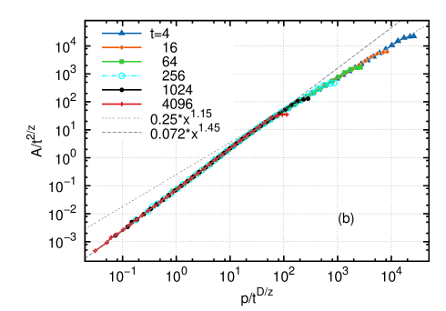
Figure 6: The hull-enclosed area against the length of the hull at different times after the critical quench for $L=400$. (a) Raw data. (b) Scaled plot. The master curve crosses over from $x^{d/D_{h}^{I}}$ to $x^{d/D_{h}^{P}}$ with $d/D_{h}^{I}\simeq 1.45$ and $d/D_{h}^{P}\simeq 1.15$.

dimension of Ising clusters’ hulls. $D_{h}/z\simeq 0.6348$ is in good agreement with the measured value and this clearly supports the idea that the growing clusters have a fractal boundary. It is interesting to notice that this does not happen in sub-critical coarsening where the domain growth is curvature-driven and the boundaries of clusters that are smaller than the cross-over scale are smooth and do not have a fractal structure (see [11] e.g. for the study of such a case in the $2d$IM). The asymptotic value, for $p/t^{D_{h}/z}\ll 1$, coincides with the expected equilibrium value, as obtained from the equilibrium simulations and shown with the (red) dashed horizontal line.

The behavior in the large scale or short time limits, $p\gg t^{D^{I}_{h}/z}$, is also interesting. Since there is a one-to-one relation between areas and perimeters, we can use $n_{h}(A,t)dA\simeq n_{h}(p,t)dp$ where $A$ and $p$ are related by eq. (19) (note that we use the same symbol $n_{h}$ to represent two different functions). Using $n_{h}(A,t)\simeq A^{-\tau}$ with $\tau=1+d/D$ for large values of $A$ and the value of the exponent $\zeta$ given in eq. (19) for large scales we find

$$n_{h}(p,t)p^{\tau^{I}_{h}}\simeq\left(\frac{p}{t^{D_{h}^{I}/z}}\right)^{\gamma}\qquad\mbox{with}\qquad\gamma=d\ \frac{D_{h}^{P}-D_{h}^{I}}{D_{h}^{P}D_{h}^{I}}=\tau_{h}^{I}-\tau_{h}^{P}$$ (20)

independently of $D$. We used the super-script $I$ to stress that the $\tau$-value in the factor in the left-hand-side corresponding to critical Ising equilibrium was used in the scaling of data in Fig. 7(b). The bump at the end of the data is just the contribution of the spanning clusters. The growing part of the master curve is very well described by the power law given above. Indeed, close to it we placed the data obtained in equilibrium at $T\to\infty$ (dashed green line) that in the representation used in the plot is given by $x^{\gamma}$, with the value of $\gamma$ given in eq. (20). The two curves are parallel in the selected range of variation (within numerical accuracy) confirming our prediction.

3.2.5 Domain area number density

We have checked that the area-hull relation for the domains conforms to the scaling in eq. (19) with the relevant $\zeta$ given by the fractal dimension of the domains.

Finally, we present the spin clusters (or domain) area distributions at several instants after the quench in Fig. 8. Again the two equilibrium distributions appear as (green and red) dashed lines. Even for the relatively short time $t=8$ MCs the change in the distribution is rather drastic, and we can observe that the system has been depleted from small clusters with area up to $80$ because of the onset of the interactions. This is related to the fact that the fractal dimension of the Ising clusters at equilibrium is greater than the dimension of the percolation clusters. Qualitatively we can explain this fact by saying that the Ising clusters are less porous because of the interactions. We perform again the rescaling of the areas by $t^{\alpha}$ and we multiply the distributions by $A^{\tau}$, with $\tau=379/187\simeq 2.027$ being the critical Ising exponent for the distribution of domain areas (see the Table). Here the best collapse (Fig. 8(b)) is obtained for the value $\alpha=0.90\ (3)$. The fractal dimension of the geometrical clusters at the critical point is $D_{c}=187/96\simeq 1.948$. Then the value of $\alpha$ is in good agreement with the value expected from scaling arguments $D_{c}/z\simeq 0.899$. Note that if we had neglected the fractal character and used $D_{c}=2$, we would have obtained $2/z\simeq 0.923$ which is also in the interval of confidence of our numerical estimate but we think the value $D_{c}/z$ with $D=187/96$ is the correct one. The scaling just discussed gives evidence for the importance of the fractal structure of the spin clusters at the critical point. The values obtained suggest a fractal front, whose fractality is the critical Ising one, propagating on increasingly larger scales and bringing the system towards a new equilibrium, although very slowly, with a law governed by the dynamic exponent $z$.

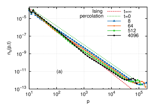
(a)

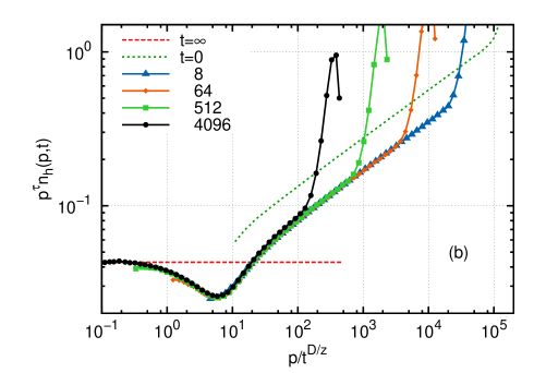
(b)

Figure 7: Time-dependent distribution of the hull length $p$ of the spin clusters, in a double logarithmic scale for the times given in the key in MCs. (a) Raw data dynamic data together with the ones for equilibrium at the departure and arrival values, $T\to\infty$ and $T_{c}$, that are shown with dashed (red and green) lines. (b) Same as in (a) but the distributions are multiplied by $p^{\tau}$ with $\tau=27/11$ the exponent of the equilibrium number density at $T_{c}$ and the lengths are divided by $t^{\alpha}$ with $\alpha=D_{h}/z\simeq 0.63$ with $D_{h}$ the fractal dimension of the equilibrium hulls at $T_{c}$.

3.3 Fortuin-Kasteleyn clusters

In this Section we present the results of simulations in which we analyze the FK clusters. These clusters are critical at $T=T_{c}$ but they are not critical at $T\to\infty$ since at infinite temperature $p=1-e^{-2\beta}=0$ and they are all composed of only one site. We constructed the dynamic FK clusters adapting the usual procedure explained in Sec. 2.3 and sketched in Fig. 1 to the time-dependent domains. At different instants after the quench from $\beta=0$ to $\beta_{c}$ we used the probability $p=1-e^{-2\beta_{c}}$ to erase bonds from the spin domains existing at the chosen times. We next studied various distribution functions associated to the FK clusters. We recall that in this study we used a square lattice for simplicity and that the initial point (infinite temperature) is not critical for the spin clusters either.

We have checked that the number density of hull-enclosed and domain FK areas as well as the area-perimeter relations satisfy the expected scaling relations already discussed for spin clusters in Sec. 3.2, so we prefer to show the data for other observables.

3.3.1 Hull length

In Fig. 10(a) we show the hull length distributions at $T\to\infty$ and at $T_{c}$ as well as the distributions of the same quantities at several times after the quench. We can easily see that the initial distribution is not a critical one since it is not a straight line in this log-log graph. As time elapses, the distribution approaches a power law behavior since it heads towards criticality. Again, to get a better description, the curves are collapsed on Fig. 10(b) by using the now usual rescaling $p^{\delta}n_{h}(p,t)=f(p/t^{\alpha})$. The best collapse onto a master curve is obtained for $\delta=2.12$ and $\alpha=0.87$. These values are compatible with $\tau=2.2$ and $D_{h}/z\simeq 0.77$, the values at the Ising critical point, cf. Table 1, though here the agreement is not as good as for the hulls of the spin clusters. We notice that for times longer than $2000$ MCs the curves do not collapse anymore for large sizes. This is expected since it roughly corresponds to the moment when the dynamical length scale reaches the order of the linear size of the system $\xi(t)\sim L$. After this time we are no longer in the regime of unconstrained domain growth as the clusters are sensitive to the finite size of the system.

3.3.2 External perimeter

The same scaling is finally applied to the external perimeter distributions of the FK clusters, the idea being to check whether the consequences of Duplantier’s duality hold out of equilibrium. The curves are not shown since they are very similar to the ones in Fig. 10. The curves collapse for $\delta=2.56$ and $\alpha=0.63$. To compare this values with the related equilibrium exponent at $T_{c}$ we must remember that, according to the duality relation evoked before [$D_{ep}(\kappa)=D_{h}(16/\kappa)$ for $\kappa\geq 4$], the external perimeters of the FK clusters at $T_{c}$ should scale at equilibrium like the hulls of the spin clusters, that is possess also at $T_{c}$ a fractal dimension $D_{ep}(\kappa=16/3)=D_{h}(\kappa=3)=11/8$. This gives $\tau\simeq 2.45$ which is compatible with $\delta$ and $\alpha=D_{ep}/z\simeq 0.63$. Therefore the relation between the statistical and geometric properties of the external perimeters of FK clusters and the hulls of spin clusters proven in equilibrium, seems to remain valid out of equilibrium for the growing FK clusters.

3.4 The interface

In the previous sections, we have seen fractal dimensions appear while considering the dynamic scaling of several probability distributions. A different strategy, that has proven to be very useful in the analysis of the equilibrium critical points and in particular in the context of the study

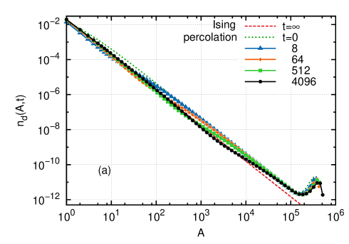
(a)

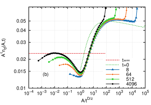
(b)

Figure 8: Time-dependent domain area distribution. (a) Raw data at the times given in the key in MCs. (b) Same as in (a) with the distributions multiplied by $A^{\tau}=A^{2.025}$ and the area rescaled by $t^{\alpha}$ with $\alpha=D/z\simeq 0.90$.

of SLE [7, 8, 9], is to study the fractal properties of an artificially generated interface. This is the line of research we follow here by generating the interface as follows. We take a $2d$IM on a triangular lattice and we quench the system from equilibrium at $T\to\infty$ to $T_{c}$ at $t=0$. With appropriate boundary conditions we force the existence of a unique curve, defined on the edges of the dual honeycomb lattice, separating spin clusters of opposite sign and going, say, from top to bottom. One such curve is shown in Fig. 9, their properties are analyzed in this section.

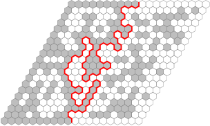
Figure 9: An interface in a $2d$IM on a triangular lattice created by imposing spin up boundary condition on the left (grey hexagons) and spin down on the right (white hexagons). The curve is defined on the edges of the dual lattice, the honeycomb lattice represented in the figure.

3.4.1 Fractal dimension

We are interested in the fractal dimension of the interface. To compute this quantity we measured the length of the curve $l(L,t)$ with $L$ the linear size of the system as a function of the time $t$. If the curve is fractal at time $t$, then the fractal dimension $d_{f}(t)$ is defined by $l(L,t)\propto L^{d_{f}(t)}$. An effective $d_{f}(t)$ is obtained from the slope of $l(L,t)$ between two sizes $L$ and $L^{\prime}$:

$$d_{f}(L,L^{\prime},t)=\frac{\ln l(L,t)-\ln l(L^{\prime},t)}{\ln L-\ln L^{\prime}}.$$ (21)

This yields a fractal dimension depending on time but also on the two lengths $L$ and $L^{\prime}$ because of finite-size corrections. In Fig. 11 we draw this fractal dimension vs. time $t$ rescaled by $L^{z}$ for several values of $L$ and $L^{\prime}$ with $z$ the dynamical exponent employed in Sec. 3.2 and Sec. 3.3.

We observe that for short times, i.e. $t\ll L^{z}$, the fractal dimension is compatible with $7/4=1.75$ the fractal dimension of the hulls at the percolation threshold, while for long times it is closer to $11/8=1.375$ the fractal dimension of the Ising clusters’ hull at the critical point. The compatibility is strong since even the finite-size corrections for the short (long) scales correspond to the related equilibrium values. The points completely on the left correspond to the initial values being rejected to $-\infty$ in the log scale. The dynamical scaling is also very accurate here since the curves perfectly collapse apart from finite-size corrections.

The main disadvantage of calculating a fractal dimension this way is having to handle the two lengths in the interpretation of the fractal dimension. This is uneasy. We use a different and more performant approach in the next subsection.

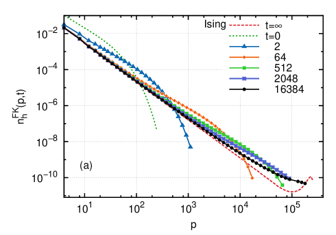
(a)

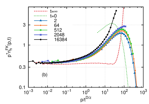
(b)

Figure 10: Number density of FK hull length $p$ at several times after the quench given in the key for a system of linear size $L=320$. (a) Raw data. (b) Same data presented in the rescaled form $p^{\tau}n^{FK}_{h}(p,t)$ vs. $p/t^{\alpha}$ with $\tau=2.12$ and $\alpha=0.87$ that gives the best data collapse.

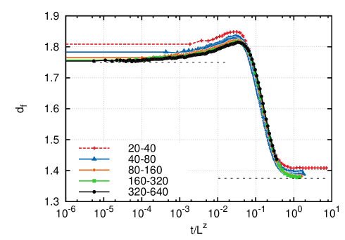
(a)

Figure 11: Fractal dimension of an interface vs. $t/L^{z}$, as deduced from eq. (21) for several couples of system sizes $L$ and $L^{\prime}=2L$ given in the key.

3.4.2 The winding angles

The percolation and Ising model hulls, at equilibrium and in the continuum limit, are conformally invariant curves described by a stochastic Loewner evolution SLE_κ with $\kappa=6$ for percolation [32] while $\kappa=3$ for Ising hulls [33, 34]. The parameter $\kappa$ can be determined numerically by computing the variance of the winding angle for two points chosen at random on a conformally invariant curve at a distance $l$ along the curve which equals

$$\langle\theta^{2}\rangle=\mbox{ct}+\frac{4(D-1)}{D}\ln l,$$ (22)

where $D$ is the fractal dimension of the curve [35, 36, 37] and ct is a constant. Finally, using eqs. (7) and (22), we obtain the following form for the variance of the winding angle:

$$\langle\theta^{2}\rangle=\mbox{ct}+\frac{4\kappa}{8+\kappa}\ln l.$$ (23)

The winding angle variance, $\langle\theta^{2}\rangle(l,t)$, is measured as a function of the distance $l$ for different times after the quench. The results for a system of linear size $L=1280$ are given in Fig. 12(a). For the time $t=0$ corresponding to percolation, a fit of the form (23) yields $\kappa=5.98$ in excellent agreement with the exact result $\kappa=6$. For the largest time simulated $t=4096$ MCs, a fit of the form (23) yields $\kappa=2.96$. For this fit we kept the data with $\ln l<6.5$ since for larger distances, the variance starts deviating from a straight line. This value is in excellent agreement with the exact result for Ising model spins clusters in equilibrium, $\kappa=3$. The best fits for $t=0$ MCs

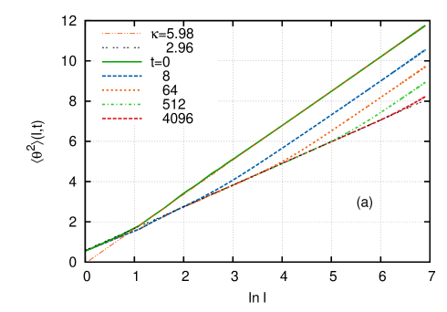
(a)

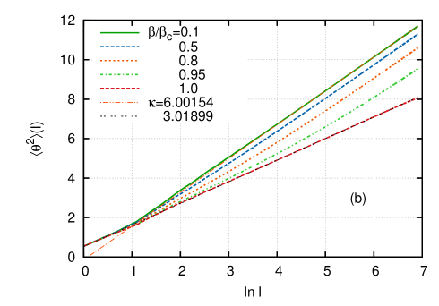
(b)

Figure 12: Variance of winding angle of interfaces out of equilibrium (a) and in equilibrium (b) for a system of linear size $L=1280$. (a) $\langle\theta^{2}\rangle$ vs. $\ln l$ for different times after the quench from $T=\infty$ to $T=T_{c}$. (b) $\langle\theta^{2}\rangle$ vs. $\ln l$ at equilibrium for different inverse temperatures $\beta=1/T$ in unit of $\beta_{c}$ given in the key.

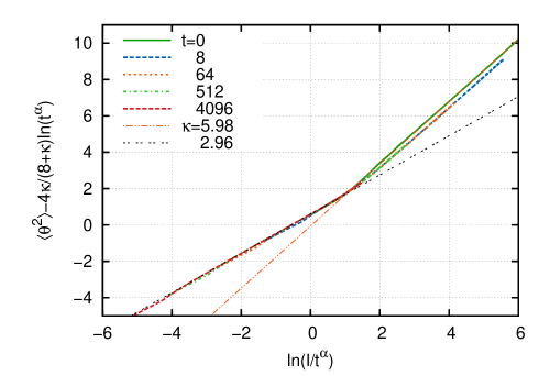
(a)

Figure 13: Same curves as in Fig. 12(a) with the rescaling $l\rightarrow l/t^{\alpha}$ and $\langle\theta^{2}\rangle(l,t)\leavevmode\nobreak\ \rightarrow\leavevmode\nobreak\ \langle\theta^{2}\rangle(l,t)\leavevmode\nobreak\ -\leavevmode\nobreak\ 4\kappa/(8+\kappa)\ln t^{\alpha}$ with $\alpha=0.65$. The dashed lines are our best fits to the small and large scale behavior and yield the $\kappa$ values given in the key.

and $t=4096$ MCs are represented as dashed lines in Fig. 12(a). We now wish to collapse these curves to make the dependence of the growing length scale upon time explicit. The length $l$ along the curve is divided by $t^{\alpha}$ and the winding angle variance corresponding to a length $t^{\alpha}$ is subtracted. Thus, in Fig. 13, we plot $\langle\theta^{2}\rangle(l,t)-4\kappa/(8+\kappa)\ln t^{\alpha}$ vs. $\ln(t/t^{\alpha})$. The curves collapse very well for $\alpha=0.65$ which is in good agreement with $D_{h}/z\simeq 0.63$ with $D_{h}=11/8$ the fractal dimension of Ising clusters’ hulls. This means that the same rescaling as the one used for the distributions works for the winding angle variance as well. In the latter case, however, the transition between the two equilibrium regimes is more rapid. Indeed, for distances smaller than the characteristic length $\xi(t)^{D_{h}}\sim t^{D_{h}/z}$ the interface is, at least for the observable $\langle\theta^{2}\rangle$, as if the system were in equilibrium at $T_{c}$ and for larger distances as if the system were still in the independent percolation regime. In the previous section, we have observed a similar crossover in the behavior of the probability distributions, with small and large scales being the ones of the initial regime of percolation and the ones of the state towards which the system is converging, respectively, but the crossover was far less abrupt.

For comparison, we present the plot of $\langle\theta^{2}\rangle$ against $\ln l$ in equilibrium for various temperatures in Fig. 12(b). It is known that the high temperature phase of the Ising model at zero field on the triangular lattice is peculiar in the sense that it is critical and in the universality class of uncorrelated percolation [38, 39]. This is not true for other planar lattices. As we have already seen, the contours of percolation clusters on the triangular lattice are described by SLE₆. This explains why for sufficiently large sizes (larger than the correlation length induced by the interactions between spins) we recover a dependence of $\langle\theta^{2}\rangle$ with $\ln l$ that is compatible with $\kappa=6$, i.e. the behavior of the interface is governed by the attractive infinite temperature point.

Both Figs. 12(a) and 12(b) are compatible with $\kappa=6$ at large scale. However, for shorter distances the behavior of the quenched and equilibrium curves are very different. In the case of the quench, for sufficiently small size and up to $l\leavevmode\nobreak\ \sim\leavevmode\nobreak\ t^{D_{h}/z}$ the curves are compatible with $\kappa=3$ (Ising spin clusters) but for the curves at equilibrium the critical Ising behavior is not observed at all.

Thus during the coarsening process the interface has a radically different behaviour from the one obtained by considering data for equilibrium at indermediate temperatures. In the first case, we flow from $T=\infty$ to $T_{c}$, with an increasing scaling length $\xi(t)\sim t^{1/z}$. In the second we flow from $T_{c}$ to $T=\infty$ with a correlation length $\xi\leavevmode\nobreak\ \sim\leavevmode\nobreak\ |T-T_{c}|^{-\nu}$ with $\nu=1$. In this second case we can only observe the critical large scale behaviour dominated by the percolation point while in the first case we distinguish two behaviors with a crossover controlled by the characteristic length $\xi(t)\leavevmode\nobreak\ \sim\leavevmode\nobreak\ t^{1/z}$.

4 Conclusion

In this paper we analyzed the dynamics of a system instantaneously quenched from one critical point to another one. We used the prototype statistical model, the $2d$ Ising model, quenched from $T\to\infty$, i.e. critical site percolation, to the Ising critical point.

As observed in [10]-[16] for sub-critical quenches, the typical growing length, $\xi(t)\simeq t^{1/z}$ in this case, separates two length scales. In the smaller one, all mesoscopic observables (areas, perimeters, etc.) satisfy the statistical and geometric properties of the working temperature equilibrium state. Instead, in the largest scale, these same observables are the ones of the initial state. In sub-critical quenches, this result could be shown analytically for the hull-enclosed area distribution [10, 13] and it was confirmed numerically for different quantities and in different systems.

The attraction of quenches between critical points is that, in the departing and arrival equilibrium conditions, very powerful analytic methods (Coulomb gas, conformal field theory, SLE) allowed one to compute a myriad of geometric properties including fractal dimensions and related critical exponents. Could these methods be extended to deduce, analytically, the results presented in this manuscript for a particular case, the $2d$ Ising model, that we conjecture apply to all critical quenches, at least in bidimensional systems? This is definitely an interesting question on which we plan to work in the future.

Acknowledgements       LFC wishes to thank to J. J. Arenzon, A. J. Bray, M. P. Loureiro, Y. Sarrazin and A. Sicilia for our earlier collaboration on similar problems. We also wish to thank J. Cardy and R. Santachiara for useful discussions on the contents of this manuscript.

References

- [1] Hohenberg P C and Halperin B I 1977 Rev. Mod. Phys. 49 435
- [2] Janssen H K 1992 From Phase Transitions to Chaos—Topics in Modern Statistical Physics (World Scientific, Singapore) p 68
- [3] Calabrese P and Gambassi A 2005 J. Phys. A: Math. Gen. 38 R133
- [4] Täuber U C Critical dynamics - A field theory approach to equilibrium and non-equilibrium scaling behavior in preparation http://www.phys.vt.edu/~tauber/
- [5] Nienhuis B 1987 Coulomb gas formulation of two dimensional phase transitions (Phase Transitions and Critical Phenomena vol 11) (Academic Press London) chap 1, p 1
- [6] Cardy J 1987 Conformal Invariance (Phase Transitions and Critical Phenomena vol 11) (Academic Press London) chap 2, p 55
- [7] Cardy J 2005 Ann. Phys. 318 81
- [8] Gruzberg I A 2006 J. Phys. A: Math. Gen. 39 12601
- [9] Bernard M and Bernard D 2006 Phys. Rep. 432 115
- [10] Arenzon J J, Bray A J, Cugliandolo L F and Sicilia A 2007 Phys. Rev. Lett. 98 8
- [11] Sicilia A, Arenzon J J, Bray A J and Cugliandolo L F 2007 Phys. Rev. E 76 061116
- [12] Barros K, Krapivsky P L and S R 2009 Phys. Rev. E 80 040101
- [13] Sicilia A, Sarrazin Y, Arenzon J J, Bray A J and Cugliandolo L F 2009 Phys. Rev. E 80 031121
- [14] Sicilia A, Arenzon J J, Bray A J and Cugliandolo L F 2008 EPL 82 10001
- [15] Loureiro M P, Arenzon J J, Cugliandolo L F and Sicilia A 2010 Phys. Rev. E 81 021129
- [16] Loureiro M P, Arenzon J J and Cugliandolo L F 2012 Phys. Rev. E 85 021135
- [17] Sykes M F and Gaunt D S 1976 J. Phys. A: Math. Gen. 9 2131
- [18] Coniglio A and Klein W 1980 J. Phys. A: Math. Gen. 13 2775
- [19] Stauffer D and Aharony A 1994 Introduction to percolation theory (Taylor & Francis)
- [20] Müller-Krumbhaar H 1974 Phys. Lett. A 50 27
- [21] Fortuin C M and Kasteleyn P W 1972 Physica 57 536
- [22] Jan N, Coniglio A and Stauffer D 1982 J. Phys. A: Math. Gen. 15 L699
- [23] Duplantier B 2000 Phys. Rev. Lett. 84 1363
- [24] Janke W and Schakel A M 2004 Nucl. Phys. B 700 385
- [25] Stella A L and Vanderzande C 1989 Phys. Rev. Lett. 62 1067
- [26] Duplantier B and Saleur H 1989 Phys. Rev. Lett. 63 2536
- [27] Picco M, Santachiara R and Sicilia A 2009 J. Stat. Mech. 2009 P04013
- [28] Cardy J and Ziff R 2003 J. Stat. Phys. 110 1
- [29] Sykes M F and Essam J W 1963 Phys. Rev. Lett. 10 3
- [30] Bausch R, Janssen H K and Wagner H 1976 Z. Phys. B 24 113
- [31] Nightingale M P and Blöte H W J 2000 Phys. Rev. B 62 1089
- [32] Smirnov S 2001 C.R.A.S. - Series I - Mathematics 333 239
- [33] Smirnov S 2006 Proc. Int. Congr. Math. 2 1421
- [34] Chelkak D and Smirnov S 2009 arXiv:0910.2045
- [35] Duplantier B and Saleur H 1988 Phys. Rev. Lett. 60 2343
- [36] Duplantier B and Binder I A 2002 Phys. Rev. Lett. 89 264101
- [37] Wieland B and Wilson D B 2003 Phys. Rev. E 68 056101
- [38] Klein W, Stanley H E, Reynolds P J and Coniglio A 1978 Phys. Rev. Lett. 41 1145
- [39] Balint A, Camia F and Meester R 2010 J. Stat. Phys. 139 122