Consensus clustering in complex networks

Abstract

The community structure of complex networks reveals both their organization and hidden relationships among their constituents. Most community detection methods currently available are not deterministic, and their results typically depend on the specific random seeds, initial conditions and tie-break rules adopted for their execution. Consensus clustering is used in data analysis to generate stable results out of a set of partitions delivered by stochastic methods. Here we show that consensus clustering can be combined with any existing method in a self-consistent way, enhancing considerably both the stability and the accuracy of the resulting partitions. This framework is also particularly suitable to monitor the evolution of community structure in temporal networks. An application of consensus clustering to a large citation network of physics papers demonstrates its capability to keep track of the birth, death and diversification of topics.

I Introduction

Network systems Albert and Barabási (2002); Dorogovtsev and Mendes (2002); Newman (2003); Pastor-Satorras and Vespignani (2004); Boccaletti et al. (2006); Caldarelli (2007); Barrat et al. (2008); Cohen and Havlin (2010) typically display a modular organization, reflecting the existence of special affinities among vertices in the same module, which may be a consequence of their having similar features or the same roles in the network. Such affinities are revealed by a considerably larger density of edges within modules than between modules. This property is called community structure or graph clustering Girvan and Newman (2002); Schaeffer (2007); Porter et al. (2009); Fortunato (2010); Newman (2012): detecting the modules (also called clusters or communities) may uncover similarity classes of vertices, the organization of the system and the function of its parts.

The community structure of complex networks is still rather elusive. The definition of community is controversial, and should be adapted to the particular class of systems/problems one considers. Consequently it is not yet clear how scholars can test and validate community detection methods, although the issue has lately received some attention Lancichinetti et al. (2008); Lancichinetti and Fortunato (2009); Lancichinetti and Fortunato (2009); Orman and Labatut (2010); Orman et al. (2011). Also, in order to deliver possibly more reliable results, methods should ideally exploit all features of the system, like edge directedness and weight (for directed and weighted networks, respectively), and account for properties of the partitions, like hierarchy Sales-Pardo et al. (2007); Clauset et al. (2008) and community overlaps Baumes et al. (2005); Palla et al. (2005). Very few methods are capable to take all these factors into consideration Rosvall and Bergstrom (2008); Lancichinetti et al. (2011). Another important barrier is the computational complexity of the algorithms, which keep many of them from being applied to networks with millions of vertices or larger.

In this paper we focus on another major problem affecting clustering techniques. Most of them, in fact, do not deliver a unique answer. The most typical scenario is when the seeked partition or individual clusters correspond to extrema of a cost function Clauset (2005); Newman (2006); Lancichinetti et al. (2009), whose search can only be carried out with approximation techniques, with results depending on random seeds and on the choice of initial conditions. Allegedly deterministic methods may also run into similar difficulties. For instance, in divisive clustering methods Girvan and Newman (2002); Radicchi et al. (2004) the edges to be removed are the ones corresponding to the lowest/highest value of a variable, and there is a non-negligible chance of ties, especially in the final stages of the calculation, when many edges have been removed from the system. In such cases one usually picks at random from the set of edges with equal (extremal) values, introducing a dependence on random seeds.

In the presence of several outputs of a given method, is there a partition more representative of the actual community structure of the system? If this were the case, one would need a criterion to sort out a specific partition and discard all others. A better option is combining the information of the different outputs into a new partition. Exploiting the information of different partitions is also very important in the detection of communities in dynamic systems Hopcroft et al. (2004); Palla et al. (2007); Mucha et al. (2010); Chakrabarti et al. (2006), a problem of growing importance, given the increasing availability of time-stamped network datasets Holme and Saramäki (2012). Existing methods typically rely on the analysis of individual snapshots, while the history of the system should also play a role Chakrabarti et al. (2006). Therefore, combining partitions corresponding to different time windows is a promising approach.

Consensus clustering Strehl and Ghosh (2002); Topchy et al. (2005); Goder and Filkov (2008) is a well known technique used in data analysis to solve this problem. Typically, the goal is searching for the so-called median (or consensus) partition, i.e. the partition that is most similar, on average, to all the input partitions. The similarity can be measured in several ways, for instance with the Normalized Mutual Information (NMI) Danon et al. (2005). In its standard formulation it is a difficult combinatorial optimization problem. An alternative greedy strategy Strehl and Ghosh (2002), which we explore here, uses the consensus matrix, i.e. a matrix based on the cooccurrence of vertices in clusters of the input partitions. The consensus matrix is used as an input for the graph clustering technique adopted, leading to a new set of partitions, which generate a new consensus matrix, etc., until a unique partition is finally reached, which cannot be altered by further iterations. This procedure has proven to lead quickly to consistent and stable partitions in real networks Kwak et al. (2011).

We stress that our goal is not finding a better optimum for the objective function of a given method. Consensus partitions usually do not deliver improved optima. On the other hand, global quality functions, like modularity Newman and Girvan (2004), are known to have serious limits Fortunato and Barthélemy (2007); Good et al. (2010); Lancichinetti and Fortunato (2011), and their optimization is often unable to detect clusters in realistic settings, not even when the clusters are loosely connected to each other. In this respect, insisting in finding the absolute optimum of the measure would not be productive. However, if we buy the popular notion of communities as subgraphs with a high internal edge density and a comparatively low external edge density, the task of any method would be easier if we managed to further increase the internal edge density of the subgraphs, enhancing their cohesion, and to further decrease the edge density between the subgraphs, enhancing their separation. Ideally, if we could push this process to the extreme, we would end up with a set of disconnected cliques, which every method would be able to identify, despite its limitations. Consensus clustering induces this type of transformation (Fig. 1) and therefore it mitigates the deficiencies of clustering algorithms, leading to more efficient techniques. The situation in a sense recalls spectral clustering von Luxburg (2006), where by mapping the original network in a network of points in a Euclidean space, through the eigenvector components of a given matrix (typically the Laplacian), one ends up with a system which is easier to clusterize.

In this paper we present the first systematic study of consensus clustering. We show that the consensus partition gets much closer to the actual community structure of the system than the partitions obtained from the direct application of the chosen clustering method. We will also see how to monitor the evolution of clusters in temporal networks, by deriving the consensus partition from several snapshots of the system. We demonstrate the power of this approach by studying the evolution of topics in the citation network of papers published by the American Physical Society (APS).

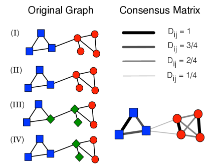
Figure 1: Effect of consensus clustering on community structure. Schematic illustration of consensus clustering on a graph with two visible clusters, whose vertices are indicated by the squares and circles on the (I) and (II) diagrams. The combination of the partitions (I), (II), (III) and (IV) yields the (weighted) consensus matrix illustrated on the right (see Methods). The thickness of each edge is proportional to its weight. In the consensus matrix the cluster structure of the original network is more visible: the two communities have become cliques, with “heavy” edges, whereas the connections between them are quite weak. Interestingly, this improvement has been achieved despite the presence of two inaccurate partitions in three clusters (III and IV).

II Results

II.1 Accuracy

In order to demonstrate the superior performance achievable by integrating consensus clustering in a given method, we tested the results on artificial benchmark graphs with built-in community structure. We chose the LFR benchmark graphs, which have become a standard in the evaluation of the performance of clustering algorithms Lancichinetti et al. (2008); Lancichinetti and Fortunato (2009); Lancichinetti and Fortunato (2009); Orman and Labatut (2010); Orman et al. (2011). The LFR benchmark is a generalization of the four-groups benchmark proposed by Girvan and Newman, which is a particular realization of the planted $\ell$-partition model by Condon and Karp Condon and Karp (2001). LFR graphs are characterized by power law distributions of vertex degree and community size, features that frequently occur in real world networks.

The clustering algorithms we used are listed below:

• Fast greedy modularity optimization. It is a technique developed by Clauset et al. Clauset et al. (2004), that performs a quick maximization of the modularity by Newman and Girvan Newman and Girvan (2004). The accuracy of the estimate for the modularity maximum is not very high, but the method has been frequently used because it has been one of the first techniques able to analyze large networks. We label it here as Clauset et al..

• Modularity optimization via simulated annealing. Here the maximization of modularity is carried out in a more exhaustive (and computationally expensive) way. Simulated annealing is a traditional technique used in global optimization problems Kirkpatrick et al. (1983). The first application to modularity has been devised by Guimerá et al. Guimerà et al. (2004). In contrast to the standard design, we start at zero temperature. This is necessary because if the method is very stable there is no point in using the consensus approach: if the algorithm systematically finds the same clusters, the consensus matrix $D$ would consist of $m$ disconnected cliques and the successive clusterization of $D$ would yield the same clusters over and over. For the method we use the label SA.

• Louvain method. The goal is still the optimization of modularity, by means of a hierarchical approach. First one partitions the original network in small communities, such to maximize modularity with respect to local moves of the vertices. This first generation clusters turn into supervertices of a (much) smaller weighted graph, where the procedure is iterated, and so on, until modularity reaches a maximum. It is a fast method, suitable to analyze very large graphs. However, like all methods based on modularity optimization, including the previous two, it is biased by the intrinsic limits of modularity maximization Fortunato and Barthélemy (2007); Good et al. (2010); Lancichinetti and Fortunato (2011). We refer to this method as to Louvain.

• Label propagation method. This method Raghavan et al. (2007) simulates the spreading of labels based on the simple rule that at each iteration a given vertex takes the most frequent label in its neighborhood. The starting configuration is chosen such that every vertex is given a different label and the procedure is iterated until convergence. This method has the problem of partitioning the network such that there are very big clusters, due to the possibility of a few labels to propagate over large portions of the graph. We considered asynchronous updates, i.e. we update the vertex memberships according to the latest memberships of the neighbors. We shall refer to this method as LPM.

• Infomap. The idea behind this method is the same as in cartography: dividing the network in areas, like counties/states in a map, and recycling the identifiers/names of vertices/towns among different areas. The goal is to minimize the description of an infinitely long random walk taking place on the network Rosvall and Bergstrom (2008). When the graph has recognizable clusters, most of the time the walker will be trapped within a cluster. That way, the additional cost of introducing new labels to identify the clusters is compensated by the fact that such labels are seldom used to describe the process, as transitions between clusters are unfrequent, so the recycling of the binary identifiers for the vertices among different clusters leads to major savings in the description of the random walk. We shall refer to this method as Infomap.

• OSLOM. The method relies on the concept of statistical significance of clusters. The idea here is that, since random graphs are not supposed to have clusters, the subgraphs of a network that are deemed to be communities should be very different from the subgraphs one observes in a random graph with similar features as the system at study. The statistical significance is then estimated through the probability of finding the observed clusters in a random network with identical expected degree sequence Lancichinetti et al. (2011). Clusters are identified by maximizing locally such probability. We shall refer to this method as OSLOM.

All the above techniques can be applied to weighted networks, a necessary requisite for our implementation of consensus clustering (see Methods).

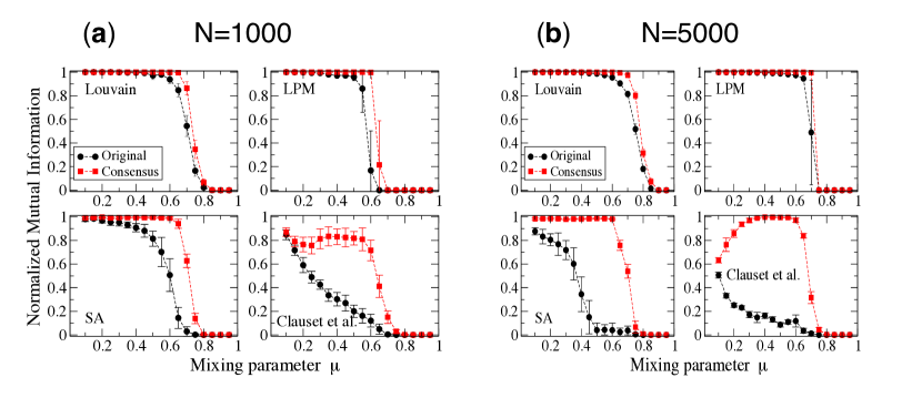
Figure 2: Consensus clustering on the LFR benchmark. The dots indicate the performance of the original method, the squares that obtained with consensus clustering. The parameters of the LFR benchmark graphs are: average degree $\langle k\rangle=20$, maximum degree $k_{max}=50$, minimum community size $c_{min}=10$, maximum community size $c_{max}=50$, the degree exponent is $\tau_{1}=2$, the community size exponent is $\tau_{2}=3$. Each panel correspond to a clustering algorithm, indicated by the label. The two sets of plots correspond to networks with $1000$ (a) and $5000$ (b) vertices.

In Fig. 2 we show the results of our tests. Each panel reports the value of the Normalized Mutual Information (NMI) between the planted partition of the benchmark and the one found by the algorithm as a function of the mixing parameter $\mu$, which is a measure of the degree of fuzziness of the clusters. Low values of $\mu$ correspond to well-separated clusters, which are fairly easy to detect; by increasing $\mu$ communities get more mixed and clustering algorithms have more difficulties to distinguish them from each other. As a consequence, all curves display a decreasing trend. The NMI equals $1$ if the two partitions to compare are identical, and approaches $0$ if they are very different. In Fig 2a and 2b the benchmark graphs consist of $1000$ and $5000$ vertices, respectively. Each point corresponds to an average over $100$ different graph realizations. For every realization we have produced $150$ partitions with the chosen algorithm. The curve “Original” shows the average of the NMI between each partition and the planted partition. The curve “Consensus” reports the NMI between the consensus and the planted partition, where the former has been derived from the $150$ input partitions. We do not show the results for Infomap and OSLOM because their performance on the LFR benchmark graphs is very good already Lancichinetti and Fortunato (2009); Lancichinetti et al. (2011), so it could not be sensibly improved by means of consensus clustering (we have verified that there still is a small improvement, though). The procedures to set the number of runs and the value of the threshold $\tau$ for each method are detailed in the Appendix. In all cases, consensus clustering leads to better partitions than those of the original method. The improvement is particularly impressive for the method by Clauset et al.: the latter is known to have a poor performance on the LFR benchmark Lancichinetti and Fortunato (2009), and yet in an intermediate range of values of the mixing parameter $\mu$ it is able to detect the right partition by composing the results of individual runs. For $\mu$ small the algorithm delivers rather stable results, so the consensus partition still differs significantly from the planted partition of the benchmark. In the Appendix we give a mathematical argument to show why consensus clustering is so effective on the LFR benchmark.

II.2 Stability

Another major advantage of consensus clustering is the fact that it leads to stable partitions Kwak et al. (2011). Here we verify how stability varies with the number of input runs $r$.

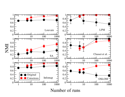
Figure 3: Stability plot for the neural network of C. elegans. The network has $453$ vertices and $2\,050$ edges.

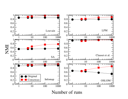
Figure 4: Stability plot for the citation network of papers published in journals of the American Physical Society (APS). The original dataset is too large to get results in a reasonable time, so the plot refers to the subset containing all papers published in $1960$ and the ones cited by them.

In Figs. 3 and 4 we present stability plots for two real world datasets: the neural network of C. elegansWhite et al. (1986); Watts and Strogatz (1998) ($453$ vertices, $2\,050$ edges); the citation network of papers published in journals of the American Physical Society (APS) ($445\,443$ vertices, $4\,505\,730$ directed edges). Each figure shows two curves: the average NMI between best partitions (circles); the average NMI between consensus partitions (squares). Both the best and the consensus partition are computed for $r$ input runs, and the procedure is repeated for $20$ sequences of $r$ runs. So we end up having $20$ best partitions and $20$ consensus partitions. The values reported are then averages over all possible pairs that one can have out of $20$ numbers. Each of the six panels corresponds to a specific clustering algorithm. To derive the consensus partitions we used the same values of the threshold parameter $\tau$ as in the tests of Fig. 2a (for Infomap and OSLOM $\tau=0.5$).

As “best” partition for Louvain, SA and Clauset et al. we take the one with largest modularity. This sounds like the most natural choice, since such methods aim at maximizing modularity. For the LPM there is no way to determine which partition could be considered the best, so we took the one with maximal modularity as well. On the other hand, both Infomap and OSLOM have the option to select the best partition out of a set of $r$ runs.

In Fig. 3 we show the stability plot for C. elegans. For all methods the consensus partition turns out to be more stable of the input than the best partition. The only exception is the method by Clauset et al., but the two curves are rather close to each other. We remark that increasing the number of input runs does not necessarily imply more stable partitions. In the cases of LPM and OSLOM, for instance, the best partitions of the method get more unstable for $r\simeq 10$. On the other hand, the stability of the consensus partition is monotonically increasing for all six algorithms.

In Fig. 4 we see the corresponding plot for the APS dataset. The analysis of the full dataset is too computationally expensive, so we focused on a subset, that of papers published in $1960$, along with the papers cited by them. The resulting network has $5\,696$ vertices and $8\,634$ edges. Again, we see that the stability of the consensus partition grows monotonically with the number of input runs $r$, and it remains higher than that of the best partition.

In the Appendix we show that the consensus partition is not only more stable, but it also has higher fidelity than the individual input partitions it combines (Figs. S5 and S6).

II.3 Dynamic communities

Consensus clustering is a powerful tool to explore the dynamics of community structure as well. Here we show that it is able to monitor the history of the citation network of the APS, and to follow birth, growth, fragmentation, decay and death of scientific topics. The procedure to derive the consensus partitions out of time snapshots of a network is described in the Methods.

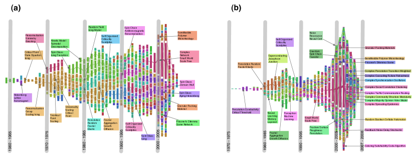
Figure 5: Time evolution of clusters in the APS citation network. In (a) we selected all the clusters that have at least one of the keywords Criticality, Fractal, Ising, Network and Renormalization among the top 15 most frequent words appearing in the title of the papers, while in (b) we just filtered the keyword Network(s). Both diagrams were obtained using Infomap on snapshots spanning each a window of $5$ years, except at the right end of each diagram: since there is no data after $2008$, the last windows must have $2008$ as upper limit, so their size shrinks ($2004-2008$, $2005-2008$, $2006-2008$, $2007-2008$). Consensus is computed by combining pairs of consecutive snapshots (see Methods). A color uniquely identifies a module, while the width of the links between clusters is proportional to the number of papers they have in common. In (b) we observe the rapid growth of the field Complex Networks, which eventually splits in a number of smaller subtopics, like Community Structure, Epidemic Spreading, Robustness, etc..

The evolution of the APS dataset is shown in Fig. 5a. The system is too large to be meaningfully displayed in a single figure, so we focused on the evolution of communities of papers in Statistical Physics. For that, we selected only the clusters whose papers include Criticality, Fractal, Ising, Network and Renormalization among the $15$ most frequent words in their titles. Each vertical bar corresponds to a time window of $5$ years (see Methods), its length to the size of the system. The time ranges from $1945$ until $2008$. The evolution is characterized by alternating phases of expansion and contraction, although in the long term there is a growing tendency in the number of papers. This is due to the fact that the keywords we selected were fashionable in different historical phases of the development of Statistical Physics, so some of them became obsolete after some time (i.e., there are less papers with those keywords), while at the same time others become more fashionable. Communities are identified by the colors. Pairs of matching clusters in consecutive times are marked by the same color. Clusters of consecutive time windows sharing papers are joined by links, whose width is proportional to the number of common papers. We mark the clusters corresponding to famous topics in Statistical Physics, indicating the most frequent words appearing in the titles of the papers of each cluster. One can spot the emergence of new fields, like Self-Organized Criticality, Spin Glasses and Complex Networks.

In Fig. 5b we consider only papers with the words Network or Networks among the $15$ most frequent words in their titles. Here we can observe the genesis of the fields Neural Networks and Complex Networks. In order to have clearer pictures, in Fig. 5a we only plotted clusters that have at least 50 papers, while in Fig. 5b the threshold is 10 papers.

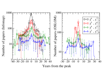
Figure 6: Evolution of average size of clusters. The time ranges of the evolution of the communities have been shifted such that the year when a cluster reaches its maximum is $0$. The two panels show the results obtained with Infomap (left) and OSLOM (right). The data are aggregated in four bins, according to the maximum size reached by the cluster. The phases of growth and decay of fields appear rather symmetric.

For a quantitative assessment of the birth, evolution and death of topics, we keep track of each cluster matching it with the most similar module in the following time frame (see Methods). This allows us to compute one sequence for each cluster, which reports its size for all the years when the community was present. In Fig. 6 we computed the statistics of these sequences, centering them on the year when the cluster reached its peak (reference year $0$). To obtain smooth patterns, clusters are aggregated in bins according to their peak magnitude. Fig. 6 shows the average cluster size for each bin as a function of the years from the peak. We computed the curves using Infomap (left) and OSLOM (right). Around the peak, the cluster sizes are highly heterogeneous, with some important topics reaching almost $1000$ papers at the peak (for Infomap). The rise and decline of topics take place around 10 years before and after the peak, with a remarkably symmetric pattern with respect to the maximum.

III Discussion

Consensus clustering is an invaluable tool to cope with the stochastic fluctuations in the results of clustering techniques. We have seen that the integration of consensus clustering with popular existing techniques leads to more accurate partitions than the ones delivered by the methods alone, in artificial graphs with planted community structure. This holds even for methods whose direct application gives poor results on the same graphs. In this way it is possible to fully exploit the power of each method and the diversity of the partitions, rather than being a problem, becomes a factor of performance enhancement.

Finding a consensus between different partitions also offers a natural solution to the problem of detecting communities in dynamic networks. Here one combines partitions corresponding to snapshots of the system, in overlapping time windows. Results depend on the choice of the amplitude of the time windows and on the number of snapshots combined in the same consensus partition. The choice of these parameters may be suggested by the specific system at study. It is usually possible to identify a meaningful time scale for the evolution of the system. In those cases both the size of the time windows and the number of snapshots to combine can be selected accordingly. As a safe guideline one should avoid merging partitions referring to a time range which is much broader than the natural time scale of the network. A good policy is to explore various possibilities and see if results are robust within ample ranges of reasonable values for the parameters. Additional complications arise from the fact that the evolution of the system may not be linear in time, so that it cannot be followed in terms of standard time units. In citation networks, like the one we studied, it is known that the number of published papers has been increasing exponentially in time. Therefore, a fixed time window would cover many more events (i.e. published papers and mutual citations) if it refers to a recent period than to some decades ago. In those cases, a natural choice could be to consider snapshots covering time windows of decreasing size.

Methods

The consensus matrix. Let us suppose that we wish to combine $n_{P}$ partitions found by a clustering algorithm on a network with $n$ vertices. The consensus matrix ${\bf D}$ is an $n\times n$ matrix, whose entry $D_{ij}$ indicates the number of partitions in which vertices $i$ and $j$ of the network were assigned to the same cluster, divided by the number of partitions $n_{P}$. The matrix ${\bf D}$ is usually much denser than the adjacency matrix ${\bf A}$ of the original network, because in the consensus matrix there is an edge between any two vertices which have cooccurred in the same cluster at least once. On the other hand, the weights are large only for those vertices which are most frequently co-clustered, whereas low weights indicate that the vertices are probably at the boundary between different (real) clusters, so their classification in the same cluster is unlikely and essentially due to noise. We wish to maintain the large weights and to drop the low ones, therefore a filtering procedure is in order. Among the other things, in the absence of filtering the consensus matrix would quickly grow into a very dense matrix, which would make the application of any clustering algorithm computationally expensive.

We discard all entries of ${\bf D}$ below a threshold $\tau$. We stress that there might be some noisy vertices whose edges could all be below the threshold, and they would be not connected anymore. When this happens, we just connect them to their neighbors with highest weights, to keep the graph connected all along the procedure.

Next we apply the same clustering algorithm to ${\bf D}$ and produce another set of partitions, which is then used to construct a new consensus matrix ${\bf D}^{\prime}$, as described above. The procedure is iterated until the consensus matrix turns into a block diagonal matrix ${\bf D}^{final}$, whose weights equal $1$ for vertices in the same block and $0$ for vertices in different blocks. The matrix ${\bf D}^{final}$ delivers the community structure of the original network. In our calculations typically one iteration is sufficient to lead to stable results. We remark that in order to use the same clustering method all along, the latter has to be able to detect clusters in weighted networks, since the consensus matrix is weighted. This is a necessary constraint on the choice of the methods for which one could use the procedure proposed here. However, it is not a severe limitation, as most clustering algorithms in the literature can handle weighted networks or can be trivially extended to deal with them.

We close by summarizing the procedure, step by step. The starting point is a network ${\cal G}$ with $n$ vertices and a clustering algorithm ${\bf A}$.

1. Apply ${\bf A}$ on ${\cal G}$ $n_{P}$ times, so to yield $n_{P}$ partitions.

2. Compute the consensus matrix ${\bf D}$, where $D_{ij}$ is the number of partitions in which vertices $i$ and $j$ of ${\cal G}$ are assigned to the same cluster, divided by $n_{P}$.

3. All entries of ${\bf D}$ below a chosen threshold $\tau$ are set to zero.

4. Apply ${\bf A}$ on ${\bf D}$ $n_{P}$ times, so to yield $n_{P}$ partitions.

5. If the partitions are all equal, stop (the consensus matrix would be block-diagonal). Otherwise go back to 2.

Consensus for dynamic clusters. In the case of temporal networks, the dynamics of the system is represented as a succession of snapshots, corresponding to overlapping time windows. Let us suppose to have $m$ windows of size $\Delta t$ for a time range going from $t_{0}$ to $t_{m}$. We separate them as $[t_{0},t_{0}+\Delta t]$, $[t_{0}+1,t_{0}+\Delta t+1]$, $[t_{0}+2,t_{0}+\Delta t+2]$, …, $[t_{m}-\Delta t,t_{m}]$. Each time window is shifted by one time unit to the right with respect to the previous one. The idea is to derive the consensus partition from subsets of $r$ consecutive snapshots, with $r$ suitably chosen. One starts by combining the first $r$ snapshots, then those from $2$ to $r+1$, and so on until the interval spanned by the last $r$ snapshots. In our calculations for the APS citation network we took $\Delta t=5$ (years), $r=2$.

There are two sources of fluctuations: 1) the ones coming from the different partitions delivered by the chosen clustering technique for a given snapshot; 2) the ones coming from the fact that the structure of the network is changing in time. The entries of the consensus matrix $D_{ij}$ are obtained by computing the number of times vertices $i$ and $j$ are clustered together, and dividing it by the number of partitions corresponding to snapshots including both vertices. This looks like a more sensible choice with respect to the one we had adopted in the static case (when we took the total number of partitions used as input for the consensus matrix), as in the evolution of a temporal network new vertices may join the system and old ones may disappear.

Once the consensus partitions for each time step have been derived, there is the problem of relating clusters at different times. We need a quantitative criterion to establish whether a cluster ${\cal C}_{t+1}$ at time $t+1$ is the evolution of a cluster ${\cal C}_{t}$ at time $t$. The correspondence is not trivial: a cluster may fragment, and thus there would be many “children” clusters at time $t+1$ for the same cluster at time $t$. In order to assign to each cluster ${\cal C}_{t}$ of the consensus partition at time $t$ one and only one cluster of the consensus partition ${\cal P}^{t+1}$ at time $t+1$ we compute the Jaccard index Jaccard (1901) between ${\cal C}_{t}$ and every cluster of ${\cal P}^{t+1}$, and pick the one which yields the largest value. The Jaccard index $J(A,B)$ between two sets $A$ and $B$ equals

$$J(A,B)=\frac{|A\cap B|}{|A\cup B|}.$$ (1)

In our case, since the snapshots generating the partitions refer to different moments of the life of the system and may not contain the same elements, the Jaccard index is computed by excluding from either cluster the vertices which are not present in both partitions. The same procedure is followed to assign to each cluster ${\cal C}_{t+1}$ of the consensus partition at time $t+1$ one and only one cluster of the consensus partition ${\cal P}^{t}$ at time $t$. In general, if cluster $A$ at time $t$ is the best match of cluster $B$ at time $t+1$, the latter may not be the best match of $A$. If it is, then we use the same color for both clusters. Otherwise there is a discontinuity in the evolution of $A$, which stops at $t$, and its best match at time $t+1$ will be considered as a newly born cluster.

Appendix A Selection of the optimal number of runs and threshold $\tau$

For any implementation of our method there are two parameters that need to be set before starting the computation: 1) the number $r$ of partitions to be combined in the consensus matrix (see Methods); 2) the threshold $\tau$ used to filter the entries of the consensus matrix, to avoid that the latter becomes too dense, slowing down the procedure. In Figs. 7 and 8 we show how these numbers are chosen. Fig. 7 displays the Normalized Mutual Information (NMI) between the consensus partition and the planted partition of the benchmark graphs used for Fig. 1, for different values of $r$ and a specific value of the mixing parameter $\mu$. Each curve corresponds to a different value for the threshold $\tau$, which equals $0$, $0.5$ and $0.7$. Each panel presents the result of a different clustering algorithm; the value of $\mu$ varies for each method because consensus is the most effective the more diverse the input partitions are. Therefore we picked the value of $\mu$ at which the original method starts failing ($\mu=0.7$ for Louvain, $\mu=0.6$ for the LPM, $\mu=0.65$ for SA and $\mu=0.4$ for Clauset et al.. From Fig. 7 we deduce that for $r\approx 50$ one reaches an optimal partition with consensus clustering, which remains stable for larger values. This seems to hold regardless of the value of the threshold parameter $\tau$. Therefore, in our tests of Fig. 1 we have taken $r$ between $50$ and $100$.

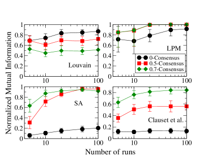
Figure 7: Accuracy of consensus clustering with the number of input runs $r$. Each panel reports the NMI between the planted partition of the LFR benchmark graphs used for Fig. 1, at a given $\mu$ (see text), as a function of the number of runs for a specific method. The symbols refer to three different choices for the threshold parameter $\tau$: $0$ (circles), $0.5$ (squares), $0.7$ (diamonds).

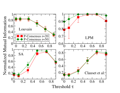
Figure 8: Accuracy of consensus clustering with the threshold parameter $\tau$. Each panel reports the NMI between the planted partition of the LFR benchmark graphs used for Fig. 7, as a function of $\tau$ for a specific method. The symbols refer to two different choices for the number of runs $r$: $20$ (squares), $50$ (diamonds).

In Fig. 8 we show instead how the threshold $\tau$ affects the results. We use the same benchmark graphs as in Fig. 7, and two values for the number of runs $r$: $20$ and $50$. The y-axis reports again the value of the NMI between the consensus and the planted partition of the benchmark. We see that the ranges of optimal values for $\tau$ depend on the clustering technique adopted. For Louvain, it is best to choose a low threshold, for the LPM $\tau$-values in the range $[0.3,0.7]$ give optimal results, for SA the best value span a shorter range (from $0.5$ to $0.7$) and for Clauset et al. the best results are obtained for fairly high values of the threshold.

Appendix B On the effectiveness of consensus clustering

To understand why consensus clustering is so effective at detecting the clusters of the LFR benchmarks, we discuss here a simpler model which resembles the LFR benchmarks. We focus on modularity optimization because it is easier to understand how consensus improves the method.

We consider a graph with $C$ cliques of $n_{c}$ vertices each. The cliques are connected by placing $C*h$ edges between randomly chosen pairs of vertices, where the vertices of each pair belong to different cliques. It can be proven that for this kind of graph, the modularity function is optimal for a partition of $\sqrt{M}$ modules of equal size, where $M$ is the number of edges. This result has been proved for a ring of cliques, but it is straightforward to verify that the same proof can be extended to this case.

Since there is a high number of combinations to group the cliques together in order to reach the optimal number of modules, we expect that, on average, each clique will be joined to some of its neighboring cliques with roughly equal probability. If we call $g$ the average number of neighboring cliques, the probability that two neighboring cliques are found in the same cluster is simply $\frac{g}{2h}$ (we recall that we placed $C*h$ links).

If $C\gg 1$ and $h$ is small enough so that the network of cliques is sparse, there will be a very small number of edges between the cliques grouped in the same module. The smallest number of edges necessary to keep $n$ vertices connected is $n-1$ (which gives a tree-like structure), and in such a case every vertex has an average degree $\langle k\rangle\approx 2$, when $n\gg 1$. In the case of a tree, we would have that $g\approx 2$. The probability for two cliques to be connected if their distance in the clique network is $d$, will be, in general,

$$p_{d}\approx\frac{1}{h(2h-1)^{d-1}}.$$ (2)

Fig. 9 shows that this approximation is not bad especially for high values of $C$. In the following plots we considered $h=10$, $n_{c}=10$.

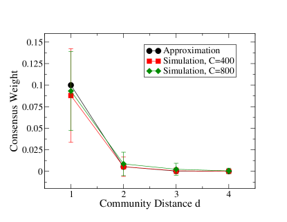
Figure 9: Probability of joining cliques in our stylized model graph with communities. Consensus weight indicates the probability that a pair of cliques are joined together. This is plotted as a function of the distance between cliques in the community network, i.e. the graph where cliques are to be seen as supervertices.

Eventually, we might expect that choosing a value of the threshold $\tau>p_{1}$, the consensus matrix will consist of $C$ disconnected cliques. Modularity optimization instead would always merge cliques together in larger clusters. Indeed, the NMI between the planted partition and the input partitions is much lower than the NMI between the planted and the consensus partition already for $\tau=0.3$ (Fig. 10).

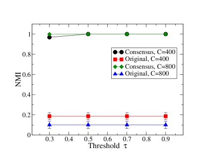
Figure 10: Fidelity of consensus partition. Normalized Mutual Information between the planted partition and the input partitions (squares and diamonds) and between the planted and the consensus partition (circles and triangles) as a function of the threshold $\tau$. We consider two values for the number of cliques of the model network, $400$ and $800$.

Appendix C Stability and fidelity of consensus partitions

In Figs. 3 and 4 we have shown that the consensus partitions are more stable than the best partitions. However trivial partitions, like the one where all vertices are together in the same cluster, would be the most stable possible, although they would be completely unrelated to the input partitions. To prove that the consensus partitions are actually very close to the input ones, Fig. 11 shows the Normalized Mutual Information of the input partitions among themselves (the average value of NMI among all pairs of different partitions) and the average value of NMI between the input partitions and the consensus partition, for different values of the threshold $\tau$, for the neural network of C. elegans. Fig. 12 shows the same plot for the APS citation network of papers published in 1960. Indeed the consensus partition is often even closer to the input partitions than the latter are to each other, with the additional advantage of being more stable. This does not hold only when the threshold is too high, because in this case the consensus partition is made of small clusters, since too many connections carry a weight under the threshold and are deleted. Otherwise this should explain why the consensus partition is more representative than the input. In Figs. 11 and 12 we considered $50$ input partitions, but the results are practically the same if we take $100$ of them.

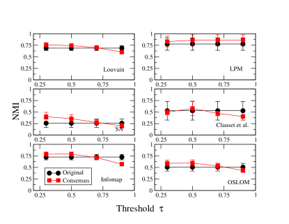
Figure 11: Fidelity of consensus partition. The black curve reports the average NMI between pairs of input partitions, the red one is the average NMI between the input partitions and the consensus one, for the neural network of C. elegans.

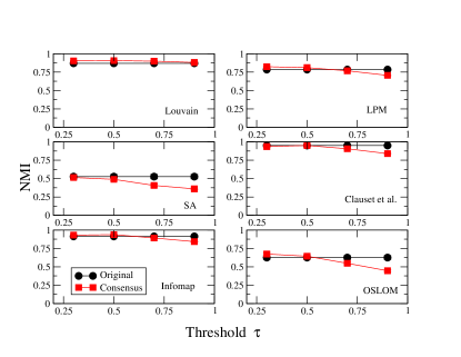
Figure 12: Fidelity of consensus partition. Same plot as Fig. 11 for a snapshot of the APS citation network, with the papers published in 1960 and those cited by them.