Theory of ultrafast quasiparticle dynamics in high-temperature superconductors: Pump fluence dependence

Abstract

We present a theory for the time-resolved optical spectroscopy of high-temperature superconductors at high excitation densities with strongly anisotropic electron-phonon coupling. A signature of the strong coupling between the out-of-plane, out-of-phase O buckling mode ($B_{1g}$) and electronic states near the antinode is observed as a higher-energy peak in the time-resolved optical conductivity and Raman spectra, while no evidence of the strong coupling between the in-plane Cu-O breathing mode and nodal electronic states is observed. More interestingly, it is observed that under appropriate conditions of pump fluence, this signature exhibits a re-entrant behavior with time delay, following the fate of the superconducting condensate.

I Introduction

Since its discovery in 1986, high-temperature superconductivity in cuprates has been a central topic of study in condensed matter physics. It is now widely believed that Cooper pair formation is essential for the superconducting condensate in these systems. However, the nature of the mediator (or glue) responsible for Cooper pairing remains hotly debated. Although the interaction of electrons with lattice vibrations is not likely to solely account for the essential properties of high-$T_{c}$ superconductors (HTSCs), many probes including angle-resolved photoemission, ALanzara:2001 ; TCuk:2004 ; TPDevereaux:2004 ; GHGweon:2004 ; WMeevasana:2006 inelastic neutron scattering, DReznik:2006 , tunneling JLee:2006 ; JXZhu:2006a and Raman MOpel:1999 spectroscopies have revealed that electron-phonon interactions have significant effects on various properties. Complementary to the time-integrated techniques, different ultrafast pump-probe techniques JDemsar:1999 ; PKusar:2008 ; RDAveritt:2002 ; EMChia:2011 ; RAKaindl:2000 ; RPSaichu:2010 have been used to disentangle microscopic interactions in HTSCs. These techniques aim to study the recombination of photoexcited quasiparticles and the resulting recovery of the superconducting condensate. In HTSCs, time-resolved (TR) angle-resolved photoemission spectroscopy LPerfetti:2007 and TR optical reflectivity NGedik:2005 have indicated that the excited quasiparticles preferentially couple to a small number of phonon subsets before decaying through anharmonic coupling to all other lattice vibrations, in support of the notion that selective optical phonon modes give rise to anisotropy of the electron-phonon (el-ph) coupling. TPDevereaux:2004 In addition, this anisotropy has also been observed in TR electron diffraction, FCarbone:2008 while resonant femtosecond study of both electronic and phononic degrees of freedom suggests strong el-ph coupling. APashkin:2010

Despite considerable progress in pump-probe experimental studies, work on microscopic modeling of the influence of el-ph interactions on observables, such as the time-dependent optical conductivity or Raman spectra, is very limited. Understanding the non-equilibrium dynamics of quantum many-body systems has, in fact, posed a theoretical challenge. Historically, theoretical attempts to model the time evolution of properties have either used quasi-equilibrium models such as $T^{*}$ and $\mu^{*}$ models EJNicol:2003 to describe non-equilibrium excitations created by a pump pulse VVKabanov:1999 or rate equation approaches based on the phenomenological Rothwarf-Taylor model ARothwarf:1967 to describe the recovery dynamics of the superconducting state. Recently, the time evolution of the optical conductivity has been studied within a microscopic model that treats the excitation and relaxation dynamics on the same footing. JUnterh:2008 All these theories are suitable for pump-probe experiments with low excitation fluence, where the superconducting condensate is merely perturbed but not destroyed. A picture of the dynamics of quasiparticles and the superconducting condensate in the photo-induced phase transition regime, CGiannetti:2009 ; MBeyer:2011 ; GLDakovski:2011 which is impulsively driven by a high excitation fluence, has as yet been beyond reach.

Here we formulate a theory for the TR optical conductivity and TR Raman scattering in HTSCs in the regime of intermediate to high intensity of pump fluence. The theory is aimed to address directly the situation where the superconducting condensate can be destroyed by pump pulse. It is based on an effective temperature model for different subsystems contributing to the response: electrons, hot phonons (i.e., out-of-plane out-of-phase O buckling $B_{1g}$ phonons and half-breathing in-plane Cu-O bond stretching phonons) that are strongly coupled to electrons, and the cold lattice. The model phenomenologically includes the effect of the pump pulse but addresses in greater depth the electron-hot phonon coupling based on a microscopic model Hamiltonian for $d$-wave superconductivity in HTSCs. This microscopic treatment goes beyond previous effective models for the normal state, PBAllen:1987 ; LPerfetti:2007 allowing us to describe the quasiparticle dynamics in both the normal and superconducting states with the same approach. Within this unified model, the time evolution of the whole set of experimental measurables can be calculated in a streamlined way. Our first test of this approach considered the $B_{1g}$ phonons as the only hot phonon mode in the calculation of the TR spectral function for a very high pump fluence. JTao:2010 In the present work, we include the half-breathing phonons as a second hot phonon mode in the calculation of the TR optical spectroscopy. Importantly, the influence of excitation density on quasiparticle dynamics in HTSCs is also investigated. Our calculations show that, in the superconducting state, in addition to the peak in the optical conductivity and Raman spectra due to the Drude response, there is another peak at higher frequencies. This high frequency peak disappears when the system evolves into the normal state, but recurs if the superconducting condensate is recovered, suggesting the significance of the superconducting gap in the TR optical properties.

The outline of the paper is as follows: In Sec. II, we lay down the effective-temperature model for the $d$-wave superconductor with electronic coupling to both $B_{1g}$ and half-breathing stretching phonon modes. The time-dependent effective temperatures for the respective subsystems are evaluated depending on the strength of pump fluence. With the obtained time-dependence of effective temperatures, the time-resolved optical conductivity and Raman spectra and their pump-fluence dependence are presented in Secs. III and IV. Finally, a conduction is given in Sec. V.

II Effective temperature model

Let us consider a two-dimensional superconductor exposed to a laser field. The model Hamiltonian can be written as JUnterh:2008 ; JTao:2010

$$H = \sum_{{\bf k}\sigma}\xi_{{\bf k}}c^{\dagger}_{{\bf k}\sigma}c_{{\bf k}\sigma}+\sum_{{\bf k}}(\Delta_{{\bf k}}c_{{\bf k}\uparrow}^{\dagger}c_{-{\bf k}\downarrow}^{\dagger}+{\rm h.c.})+\sum_{{\bf q}\nu}\hbar\Omega_{\nu{\bf q}}$$ (1)

$$\times \bigg{(}b_{\nu{\bf q}}^{\dagger}b_{\nu{\bf q}}+\frac{1}{2}\bigg{)}+\frac{1}{\sqrt{N_{L}}}\sum_{{\bf k}{\bf q}\nu\sigma}g_{\nu}({\bf k},{\bf q})c^{\dagger}_{{\bf k}+{\bf q},\sigma}c_{{\bf k}\sigma}A_{\nu{\bf q}}$$

$$+ H_{\rm field}(\tau),$$

where $c^{\dagger}_{{\bf k}\sigma}$ ($b_{\nu{\bf q}}^{\dagger}$) and $c_{{\bf k}\sigma}$ ($b_{\nu{\bf q}}$) are the creation and annihilation operators for an electron with momentum $\mathbf{k}$ and spin $\sigma$ (phonon with momentum $\mathbf{q}$ and vibrational mode $\nu$; $\nu=1,2$ represent the $B_{1g}$ and half-breathing modes, respectively), $A_{\nu{\bf q}}=b_{\nu,-{\bf q}}^{\dagger}+b_{\nu{\bf q}}$, $\xi_{\mathbf{k}}$ is the normal-state energy dispersion, $\mu$ the chemical potential, $\Delta_{\bf k}=(\Delta_{0}/2)(\cos k_{x}-\cos k_{y})$ is the $d_{x^{2}-y^{2}}$-wave gap function, $N_{L}$ is the total number of lattice sites, and $g_{\nu}$ the coupling matrix. Following the procedure sketched in Ref. JTao:2010, , we arrive at a four-temperature model:

$$\frac{\partial T_{e}}{\partial\tau} = \frac{1}{C_{e}}\sum_{\nu}K_{\nu}(T_{e},T_{ph,\nu})+\frac{P_{e}}{C_{e}}\;,$$ (2a)

$$\frac{\partial T_{ph,\nu}}{\partial\tau} = -\frac{K_{\nu}(T_{e},T_{ph,\nu})}{C_{ph,\nu}}-\frac{T_{ph,\nu}-T_{l}}{\tau_{\beta,\nu}}\;,$$ (2b)

$$\frac{\partial T_{l}}{\partial\tau} = \sum_{\nu}\bigg{(}\frac{C_{ph,\nu}}{C_{l}}\bigg{)}\frac{T_{ph,\nu}-T_{l}}{\tau_{\beta,\nu}}\;.$$ (2c)

Here $K_{\nu}$ is the el-ph coupling kernel, which can be calculated from the model Hamiltonian (1) with the equation-of-motion approach. It is given by

$$K_{\nu} = \frac{4\pi}{N_{L}}\sum_{{\bf k}{\bf q}}g_{\nu}^{2}(u_{\bf k}u_{{\bf k}-{\bf q}}-v_{\bf k}v_{{\bf k}-{\bf q}})^{2}\delta(E_{{\bf k}-{\bf q}}-E_{\bf k}-\Omega_{\nu{\bf q}})$$ (3)

$$\times \Omega_{\nu{\bf q}}\bigg{[}e^{(\beta_{ph}-\beta_{e})\Omega_{\nu{\bf q}}}-1\bigg{]}f_{\mathbf{k}}(1-f_{\mathbf{k}-\mathbf{q}})N_{\Omega_{\nu{\bf q}}}\;,$$

where the Bogoliubov amplitudes are $u_{{\bf k}}=[(1+\xi_{\bf k}/E_{\bf k})/2]^{1/2}$ and $v_{\bf k}=\text{sgn}(\Delta_{{\bf k}})[(1-\xi_{\bf k}/E_{\bf k})/2]^{1/2}$ with $E_{\bf k}=\sqrt{\xi_{\bf k}^{2}+\Delta_{\bf k}^{2}}$ being the quasiparticle energy, and the Fermi-Dirac and Bose-Einstein distribution functions are given by $f_{\mathbf{k}}=f(E_{\bf k})=1/(e^{\beta_{e}E_{\bf k}}+1)$, and $N_{\Omega_{0}}=N(\Omega_{0})=1/(e^{\beta_{ph}\Omega_{0}}-1)$ with $\beta_{e(ph,\nu)}=1/k_{B}T_{e(ph,\nu)}$. In Eq. (2), the specific heat for electrons per unit cell is found to be

$$C_{e}=\frac{\beta_{e}k_{B}}{N_{L}}\sum_{\bf k}\bigg{[}-\frac{\partial f(E_{\bf k})}{\partial E_{\bf k}}\bigg{]}\bigg{(}2E_{\bf k}^{2}+\beta_{e}\Delta_{k}\frac{\partial\Delta_{k}}{\partial\beta_{e}}\bigg{)}\;,$$ (4)

while that for each hot phonon mode is given by

$$C_{ph,\nu}=\frac{k_{B}}{4}(\hbar\Omega_{\nu}\beta_{ph,\nu})^{2}\bigg{[}{\rm coth}^{2}\bigg{(}\frac{\hbar\Omega_{\nu}\beta_{ph,\nu}}{2}\bigg{)}-1\bigg{]}\;$$ (5)

in the Einstein mode approximation $\Omega_{\nu{\bf q}}=\Omega_{\nu}$. Finally, $P_{e}$ is the power intensity (i.e., power per unit cell) for pumping electrons and $\tau_{\beta\nu}$ the anharmonic decay time of each hot phonon mode.

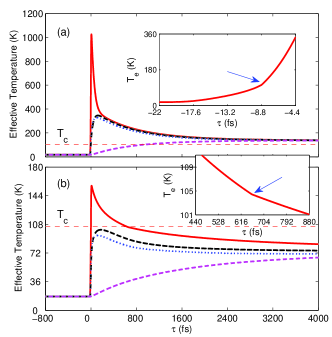
Figure 1: (Color online) Time evolution of effective temperatures of electrons $T_{e}$ (red-solid line), $B_{1g}$-phonon mode $T_{ph,1}$ (blue-dotted line), half-breathing phonon mode $T_{ph,2}$ (black-dashed line), and cold lattice $T_{l}$ (magenta-dashed line) for the powers (a) $P_{0}=0.436\;\mu\text{W}$ and (b) $P_{0}=0.022\;\mu\text{W}$. The inset in panel (a) shows a zoomed-in view of $T_{e}$ rising up above $T_{c}$, while that in panel (b) shows an enlarged view of $T_{e}$ cooling down below $T_{c}$.

Throughout the paper, we use a five-parameter tight-binding model MRNorman:1995 to describe the normal-state energy dispersion, which is typical to the optimally doped Bi₂Sr₂CaCu₂O_8+x (Bi-2212):

$$\xi_{\mathbf{k}} = -2t(\cos k_{x}+\cos k_{y})-4t^{\prime}\cos k_{x}\cos k_{y}$$ (6)

$$-2t^{\prime\prime}(\cos 2k_{x}+\cos 2k_{y})$$

$$-4t^{\prime\prime\prime}(\cos 2k_{x}\cos k_{y}+\cos k_{x}\cos 2k_{y})$$

$$-4t^{\prime\prime\prime\prime}\cos 2k_{x}\cos 2k_{y}-\mu\;,$$

where the hopping integrals $t=1$, $t^{\prime}=-0.2749$, $t^{\prime\prime}=0.0872$, $t^{\prime\prime\prime}=0.0938$, $t^{\prime\prime\prime\prime}=-0.0857$, and $\mu=-0.8772$. The absolute energy of $t$ is 150 meV. A feature of this dispersion is a flat band with a saddle point at the $M$ points of the Brillouin zone. The temperature-dependence of the $d$-wave gap magnitude is given by FGross:1986

$$\Delta_{0}(T_{e})=\Delta_{00}{\rm tanh}\{(\pi/z)\sqrt{ar(T_{c}/T_{e}-1)}\}\;,$$ (7)

where $z=\Delta_{00}/(k_{B}T_{c})$. In our calculations, we set $\Delta_{00}=30\;\text{meV}$, the critical temperature $T_{c}=104\;\text{K}$ (from the setting of $T_{c}=0.06t$ for simplicity), the specific heat jump at $T_{c}$ is $r=\Delta C_{e}/C_{e}\sim 1.43$, and $a=2/3$. We take the anisotropic el-ph coupling in the form given in Refs. TPDevereaux:2004, ; JXZhu:2006b, with $\Omega_{1}=45\;\text{meV}$ and $g_{1}^{(0)}=90\;\text{meV}$ and $\Omega_{2}=70\;\text{meV}$ and $g_{2}^{(0)}=120\;\text{meV}$, $\tau_{\beta,1}=\tau_{\beta,2}=880\;\text{fs}$, and $C_{ph,1}=C_{ph,2}=0.2C_{l}$. The pump is represented by a Gaussian pulse $P=P_{0}e^{-\tau^{2}/(2\sigma^{2})}$, with a FWHM (full width at half maximum) of 2.35 $\sigma$. Hereafter, we set $\sigma=4.4\;\text{fs}$, giving a FWHM of about 10.34 fs. This value is smaller than the commonly used experimental values of about 30-50 fs but is indeed close to that value of 12 fs used in the recent TR experiment on YBa₂Cu₃O_7-δ. APashkin:2010 We believe that this variation will not affect the qualitative physics, as will be presented below. We take the number of $\mathbf{k}$ points to be $40\times 40$ in the Brillouin zone for the temperature evolution and use $256\times 256$ for the TR optical conductivity and Raman scattering spectral function. All calculations are done with the system initially in the superconducting state, for $T\ll T_{c}$.

Figure 1 shows the time evolution of the effective temperature for each subsystem for (a) a large pump power intensity $P_{0}=0.436\;\mu\text{W}$ and (b) an intermediate value of $P_{0}=0.022\;\mu\text{W}$. These values of pump power corresponds to $120\;\mu\text{J}/\text{cm}^{2}$ and $6\;\mu\text{J}/\text{cm}^{2}$ of pump fluence in Bi-2212 by assuming a 60 nm of optical absorption depth. Starting from the initial temperature $T_{e}=T_{ph,\nu}=T_{l}=17\;\text{K}$, the electron temperature $T_{e}$ increases rapidly after photoexcitation, and the superconductor is driven into the normal state while exhibiting a kink structure at $T_{c}$ (inset of Fig. 1(a)) for both power intensities. In addition, $T_{e}$ shows a very narrow peak for the large $P_{0}$ (see Fig. 1(a)), with a broader peak for the intermediate $P_{0}$ (see Fig. 1(b)), due to the fact that the highest temperature achieved by electrons is very sensitive to the pump fluence. In both cases, the hot phonon subsystems are first heated up through their coupling to the photoexcited electrons, and after reaching their maximum temperature, they cool down by dissipating energy into the cold lattice through anharmonic coupling. A noticeable difference between the large and intermediate pump fluences is that in the latter case, the superconducting state recovers more rapidly (i.e., $T_{e}\leq T_{c}$) in a very short time ($\sim 650\;\text{fs}$), with the kink recurring during the cooling stage (inset of Fig. 1(b)). Further energy relaxation is then slowed down significantly due to the opening of the superconducting gap.

III Time-resolved optical conductivity

Within the Kubo formalism, the real part of the TR optical conductivity is given by: FMarsiglio:1991

$$\sigma_{1}(\omega)=-\frac{e^{2}{\rm Im}\Pi(\omega)}{\omega}\;,$$ (8)

where

$${\rm Im}\Pi(\omega)=-\frac{2\pi^{2}}{N_{L}}\sum_{\bf k}\biggl{(}\frac{\partial\xi_{\bf k}}{\partial k_{x}}\biggr{)}^{2}I_{\Pi}({\bf k},\omega)\;,$$ (9)

and

$$I_{\Pi}({\bf k},\omega) = 2i\int d\tau^{\prime}\text{Tr}\text{Im}[{\hat{F}}^{*}({\bf k},\tau^{\prime}){\hat{A}}({\bf k},\tau^{\prime})]e^{i\omega\tau^{\prime}}\;.$$ (10)

Here ${\hat{A}}({\bf k},\tau^{\prime})$ and ${\hat{F}}({\bf k},\tau^{\prime})$ are the Fourier transform of the TR spectral functions ${\hat{A}}({\bf k},\epsilon)$ and ${\hat{F}}({\bf k},\epsilon)\equiv{\hat{A}}({\bf k},\epsilon)f(\epsilon)$. In the derivation of Eq. (9), we have used the Hilbert transform

$$\hat{g}({\bf k},i\omega_{n})=\int_{-\infty}^{\infty}d\epsilon\frac{{\hat{A}}({\bf k},\epsilon)}{i\omega_{n}-\epsilon}\;,$$ (11)

with the single-particle spectral function

$${\hat{A}}({\bf k},\epsilon)=-\frac{1}{\pi}~{}{\rm Im}[{\hat{g}}({\bf k},i\omega_{n}\rightarrow\epsilon+i\delta)]\;,$$ (12)

where the Green’s function ${\hat{g}}$ and $\hat{A}$ are $2\times 2$ matrices in the Nambu space. Since this spectral function as calculated with the method of Ref. JTao:2010, is a function of the effective electronic temperature, which is time dependent (see the discussion in Sec. II), it is time resolved. Therefore, the optical conductivity and the Raman spectra as discussed in the next section are also time dependent.

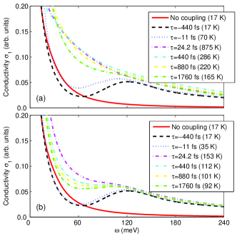
Figure 2: (Color online) Real part of the time-resolved optical conductivity at several different time delays for (a) $P_{0}=0.436\;\mu\text{W}$ and (b) $0.022\;\mu\text{W}$. The number in parentheses is $T_{e}$.

Figure 2 shows the time evolution of the real part of the optical conductivity $\sigma_{1}(\omega)$ at several selected time delays. From Fig. 2, one can see that at all time delays, the optical conductivity shows the well-known Drude peak at $\omega=0$, due to the nodal quasiparticles for the $d$-wave gap symmetry. In addition, for $\tau=-440$ fs and $-11$ fs, at which the material is superconducting and $\Delta_{0}\approx 30$ meV, we observe that $\sigma_{1}(\omega)$ exhibits a broad peak at about $\omega=2\Delta_{0}+\Omega_{ph,1}$. (The specific location may be affected by several factors, although $2\Delta_{0}+\Omega_{ph,1}$ plays a substantial role.) Our observation is consistent with earlier study of optical conductivity in the thermal equilibrium state of HTSCs. SMaiti:2010 In contrast, no peak at $\omega=\Omega_{ph,2}$ is observed (a signature of the coupling between electrons and the half-breathing mode along the nodal directions). This is due to the fact that the coupling between electrons and the $B_{1g}$ phonon mode is the strongest at the $M$ points, at which the van Hove singularity is also located. This is further verified by the observation that no such peak appears when the el-ph coupling is turned off in the initial superconducting state $T_{e}=17\;\text{K}$ (red solid line in Fig. 2). After photoexcitation, the superconducting gap, with its time-dependence encoded in the effective electron temperature $\Delta_{0}(T_{e})$, is decreased and the high-frequency peak shifts toward lower frequencies, merging into the zero-frequency Drude peak in the normal state. For large $P_{0}$, the Drude peak remains for the whole time-delay range being simulated. However, for intermediate $P_{0}$, once the superconducting condensate recovers, the ($2\Delta_{0}(T_{e})+\Omega_{ph,1}$)-peak recurs— a re-entrant behavior. The absence of the peak at $\Omega_{ph,2}$ is robust with time delay.

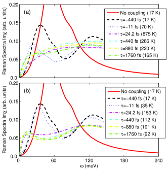
Figure 3: (Color online) Time-resolved Raman scattering spectrum at several different time delays for (a) $P_{0}=0.436\;\mu\text{W}$ and (b) $0.022\;\mu\text{W}$. The number in parentheses is $T_{e}$.

IV Time-resolved Raman scattering spectrum

The time-resolved Raman scattering intensity is calculated via a simple relation MBakr:2009 from the imaginary part of the Raman response function. In the bare vertex approximation, TPDevereaux:1994 ; TPDevereaux:2007 it is found as:

$$\text{Im}\chi(i\Omega_{m}\rightarrow\omega+i\delta)=-\frac{2\pi^{2}}{N_{L}}\sum_{\bf k}\gamma_{\bf k}^{2}I_{\chi}({\bf k},\omega)\;,$$ (13)

where

$$I_{\chi}({\bf k},\omega)=2i\int d\tau^{\prime}~{}\text{Tr}\text{Im}[\hat{\tau}_{3}{\hat{F}}^{*}({\bf k},\tau^{\prime})\hat{\tau}_{3}{\hat{A}}({\bf k},\tau^{\prime})]e^{i\omega\tau^{\prime}}.$$ (14)

Here ${\hat{\gamma}}_{\bf k}$ is the nonresonant bare Raman vertex given by ${\hat{\gamma}}_{\bf k}=\gamma_{\bf k}{\hat{\tau}}_{3}$ with ${\hat{\tau}}_{3}$ being the Pauli matrix and $\gamma_{\bf k}=\sum_{\alpha,\beta}e_{\alpha}^{S}\frac{\partial^{2}\xi_{\bf k}}{\partial k_{\alpha}\partial k_{\beta}}e_{\beta}^{I}$. ${\bf e}^{I,S}$ are the polarization unit vectors of the incident and scattered photons, and $\xi_{\bf k}$ the electronic normal-state dispersion of the conduction band.

Figure 3 shows the time evolution of the Raman scattering spectrum. When the electron-hot phonon coupling is switched off, the Raman spectrum rises with $\omega$ and has a large peak at twice the gap, $2\Delta_{0}$, at the initial temperature (red solid line in Fig. 3). A small shoulder in the curve around 90 meV arises due to the van Hove singularity. In the presence of the electron-hot phonon coupling, the superconducting gap function is renormalized, which shifts the original $2\Delta_{0}$-peak to lower frequencies. Simultaneously, another peak develops at $2\Delta_{0}+\Omega_{ph,1}$ but no peak develops at $\Omega_{ph,2}$, for the same reason for the optical conductivity (Fig. 2). After photoexcitation, this double-peak structure evolves into a very broad peak as the system enters the normal state. For large $P_{0}$, this broad peak remains for a few picoseconds. However, for intermediate $P_{0}$, once the superconducting state recovers, the double-peak structure appears again. This result is fully consistent with our calculations of the TR optical conductivity described above.

V Conclusion

We have presented a theory for the time-resolved optical conductivity and Raman spectrum, based on the TR spectral function that we have recently formulated for HTSCs. Our calculations show that the signature of the electron-$B_{1g}$ mode coupling in the TR optical conductivity and Raman spectrum is more pronounced than the consequence of the coupling between electrons and the half breathing mode. This is the result of a concurrence of anisotropy of the el-ph coupling, band structure, and $d$-wave energy gap in HTSCs. Even more interestingly, this signature also shows a re-entrant behavior in concurrence with the superconducting condensate, which can be controlled by the pump fluence. The observation of the broad peak in the TR Raman spectra and their re-entrant behavior provides a direct evidence of the el-ph coupling.

- (1) A. Lanzara, P. V. Bogdanov, X. J. Zhou, S. A. Kellar, D. L. Feng, E. D. Lu, T. Yoshida, H. Eisaki, A. Fujimori, K. Kishio, J. -I. Shimoyama, T. Noda, S. Uchida, Z. Hussain and Z. X. Shen, Nature (London) 412, 510 (2004).
- (2) T. Cuk, F. Baumberger, D. H. Lu, N. Ingle, X. J. Zhou, H. Eisaki, N. Kaneko, Z. Hussain, T. P. Devereaux, N. Nagaosa, and Z.-X. Shen, Phys. Rev. Lett. 93, 117003 (2004).
- (3) T. P. Devereaux, T. Cuk, Z.-X. Shen, and N. Nagaosa, Phys. Rev. Lett. 93, 117004 (2004).
- (4) G. H. Gweon, T. Sasagawa, S. Y. Zhou, J. Graf, H. Takagi, D. H. Lee, and A. Lanzara, Nature (Londo) 430, 187 (2004).
- (5) W. Meevasana, N. J. C. Ingle, D. H. Lu, J. R. Shi, F. Baumberger, K. M. Shen, W. S. Lee, T. Cuk, H. Eisaki, T. P. Devereaux, N. Nagaosa, J. Zaanen, and Z.-X. Shen, Phys. Rev. Lett. 96, 157003 (2006).
- (6) D. Reznik, L. Pintschovius, M. Ito, S. Iikubo, M. Sato, H. Goka, M. Fujita, K. Yamada, G. D. Gu, and J. M. Tranquada, Nature (London) 440, 1170 (2006).
- (7) J. Lee, K. Fujita, K. McElroy, J. A. Slezak, M. Wang, Y. Aiura, H. Bando, M. Ishikado, T. Masui, J.-X. Zhu, A. V. Balatsky, H. Eisaki, S. Uchida, and J. C. Davis, Nature (London) 442, 546 (2006).
- (8) J.-X. Zhu, K. McElroy, J. Lee, T. P. Devereaux, Qimiao Si, J. C. Davis, and A. V. Balatsky, Phys. Rev. Lett. 97, 177001 (2006).
- (9) M. Opel, R. Hackl, T. P. Devereaux, A. Virosztek, A. Zawadowski, A. Erb, E. Walker, H. Berger, and L. Forró, Phys. Rev. B 60, 9836 (1999).
- (10) J. Demsar, B. Podobnik, V. V. Kabanov, Th. Wolf, and D. Mihailovic, Phys. Rev. Lett. 82, 4918 (1999).
- (11) P. Kusar, V. V. Kabanov, J. Demsar, T. Mertelj, S. Sugai, and D. Mihailovic, Phys. Rev. Lett. 101, 227001 (2008).
- (12) R. D. Averitt and A.J. Taylor, J. Phys.: Condens. Matter 14, R1357 (2002).
- (13) E. E. M. Chia, J.-X. Zhu, D. Talbayev, and A. J. Taylor, Physica Status Solidi RRL 5, 1 (2011).
- (14) R. A. Kaindl, M. Woerner, T. Elsaesser, D. C. Smith, J. F. Ryan, G. A. Farnan, M. P. McCurry, D. G. Walmsley, Science 287, 470 (2000).
- (15) R. P. Saichu, I. Mahns, A. Goos, S. Binder, P. May, S. G. Singer, B. Schulz, A. Rusydi, J. Unterhinninghofen, D. Manske, P. Guptasarma, M. S. Williamsen, and M. Rübhausen, Phys. Rev. Lett. 102, 177004 (2009).
- (16) L. Perfetti, P. A. Loukakos, M. Lisowski, U. Bovensiepen, H. Eisaki, and M. Wolf, Phys. Rev. Lett. 99, 197001 (2007).
- (17) N. Gedik, M. Langner, J. Orenstein, S. Ono, Yasushi Abe, and Yoichi Ando, Phys. Rev. Lett. 95, 117005 (2005).
- (18) F. Carbone, Ding-Shyue Yang, Enrico Giannini, and Ahmed H. Zewail Proc. Natl. Acad. Sci. 105, 20161 (2008).
- (19) A. Pashkin, M. Porer, M. Beyer, K. W. Kim, A. Dubroka, C. Bernhard, X. Yao, Y. Dagan, R. Hackl, A. Erb, J. Demsar, R. Huber, and A. Leitenstorfer, Phys. Rev. Lett. 105, 067001 (2010).
- (20) E. J. Nicol and J. P. Carbotte, Phys. Rev. B 67, 214506 (2003).
- (21) V. V. Kabanov, J. Demsar, B. Podobnik, and D. Mihailovic, Phys. Rev. B 59, 1497 (1999).
- (22) A. Rothwarf and B. N. Taylor, Phys. Rev. Lett. 19, 27 (1967).
- (23) J. Unterhinninghofen, D. Manske, and A. Knorr, Phys. Rev. B 77, 180509(R) (2008).
- (24) Claudio. Giannetti, Giacomo Coslovich, Federico Cilento, Gabriele Ferrini, Hiroshi Eisaki, Nobuhisa Kaneko, Martin Greven, and Fulvio Parmigiani, Phys. Rev. B 79, 224502 (2009).
- (25) M. Beyer, D. Städter, M. Beck, H. Schäfer, V. V. Kabanov, G. Logvenov, I. Bozovic, G. Koren, and J. Demsar, Phys. Rev. B 83, 214515 (2011).
- (26) G. L. Dakovski et al. (unpublished).
- (27) P. B. Allen, Phys. Rev. Lett. 59, 1460 (1987).
- (28) J. Tao and J.-X. Zhu, Phys. Rev. B 81, 224506 (2010).
- (29) M.R. Norman, M. Randeria, H. Ding, and J. C. Campuzano, Phys. Rev. B 52, 615 (1995).
- (30) F. Gross, B.S. Chandrasekhar, D. Einzel, K. Andres, P.J. Hirschfeld, H.R. Ott, J. Beuers, Z. Fisk, and J.L. Smith, Z. Phys. B 64, 175 (1986).
- (31) J.-X. Zhu, A.V. Balatsky, T.P. Devereaux, Q. Si, J. Lee, K. McElroy, and J.C. Davis, Phys. Rev. B 73, 014511 (2006).
- (32) F. Marsiglio, Phys. Rev. B 44, 5373 (1991).
- (33) S. Maiti and A. V. Chubukov, Phys. Rev. B 81, 245111 (2010).
- (34) M. Bakr, A. P. Schnyder, L. Klam, D. Manske, C. T. Lin, B. Keimer, M. Cardona, and C. Ulrich, Phys. Rev. B 80, 064505 (2009).
- (35) T.P. Devereaux, D. Einzel, B. Stadlober, R. Hackl, D. H. Leach, and J. J. Neumeier, Phys. Rev. Lett. 72, 396 (1994).
- (36) T.P. Devereaux and R. Hackl, Rev. Mod. Phys. 79, 175 (2007).