Pairing and radio-frequency spectroscopy in two-dimensional Fermi gases

Abstract

We theoretically study the normal phase properties of strongly interacting two-component Fermi gases in two spatial dimensions. In the limit of weak attraction, we find that the gas can be described in terms of effective polarons. As the attraction between fermions increases, we find a crossover from a gas of non-interacting polarons to a pseudogap regime. We investigate how this crossover is manifested in the radio-frequency (rf) spectroscopy. Our findings qualitatively explain the differences in the recent rf spectroscopy measurements of two-dimensional Fermi gases [Sommer et al., Phys. Rev. Lett. 108, 045302 (2012) and Zhang et al., Phys. Rev. Lett. 108, 235302 (2012)].

I Introduction

Pairing of fermions in two spatial dimensions has become one of the main themes in condensed-matter physics due to the discovery of high-temperature superconductivity in copper oxide compounds Abrahams (2010). Ultracold gases of fermionic atoms provide a flexible platform for testing the various pairing mechanisms. Advances in manipulating atoms in optical lattices can ultimately lead to direct simulation of materials relevant to high-temperature superconductivity. To achieve this milestone, one first needs to understand pairing in simpler systems, such as Fermi gases confined to continuous two-dimensional (2D) geometries. Several recent experiments have probed different aspects of strongly interacting 2D Fermi gases, ranging from polaron physics Fröhlich et al. (2011); Koschorreck et al. (2012); Zhang et al. (2012) to pairing and confinement-induced molecules Dyke et al. (2011); Sommer et al. (2012); Feld et al. (2011); Baur et al. (2012). Another interesting direction is a dimensional crossover from two dimensions to three dimensions Dyke et al. (2011); Sommer et al. (2012).

One of the intriguing aspects of both high-temperature superconductors and atomic Fermi gases is the possible existence of preformed Cooper pairs above the superfluid transition temperature Abrahams (2010); Loktev et al. (2001); Perali et al. (2002); Rohe and Metzner (2001); Hu et al. (2010); Tsuchiya et al. (2009); Chien et al. (2010). This regime is referred to as the pseudogap phase, and in the context of Fermi gases, the properties of the pseudogap regime have been experimentally probed in both two-dimensional and three-dimensional (3D) systems Gaebler et al. (2010); Perali et al. (2011); Feld et al. (2011); Stewart et al. (2008). The nature of the normal state of a strongly interacting Fermi gas is still an open question since it can also be interpreted in terms of the Fermi-liquid framework Nascimbène et al. (2011). Furthermore, recent experiments have suggested that a 2D Fermi gas can be described as a gas of noninteracting polarons even in the absence of any population imbalance Zhang et al. (2012), while other experiments indicate the existence of confinement-induced molecules in the normal phase Sommer et al. (2012).

In this work, we probe the properties of the normal state of strongly interacting 2D Fermi gases. In particular, we aim to qualitatively explain the differences in the recent experiments performed in the Zwierlein group at Massachusetts Institute of Technology (MIT) Sommer et al. (2012) and in the Thomas group at North Carolina State University (NCSU) Zhang et al. (2012). We find that the normal state of weakly attractive Fermi gases can be described in terms of effective polarons, whereas strongly attractive Fermi gases are characterized by a Bardeen-Cooper-Schrieffer (BCS) -like effective dispersion and suppression of a single-particle density of states (DOS) near the Fermi energy. Such characteristics are commonly attributed to the pseudogap regime Perali et al. (2002); Stewart et al. (2008); Tsuchiya et al. (2009); Haussmann et al. (2009); Hu et al. (2010); Gaebler et al. (2010); Mueller (2011). Our analysis suggests a crossover from a gas of non-interacting polarons to the pseudogap regime with increasing attraction and qualitatively explains the different experimental results reported in Refs. Sommer et al. (2012); Zhang et al. (2012). We note that the earlier experiments reported in Ref. Fröhlich et al. (2011) regarding molecule formation in 2D Fermi gases have already been interpreted in terms of dynamically created polarons Schmidt et al. (2012) and therefore we do not discuss this experiment in the present work.

The experiments reported in Refs. Sommer et al. (2012); Zhang et al. (2012) used radio-frequency (rf) spectroscopy to probe the properties of 2D Fermi gases. Both experiments can be schematically described by an interacting, population balanced initial mixture of spin-$\uparrow$ and spin-$\downarrow$ atoms. A short rf pulse is applied to convert spin-$\downarrow$ atoms into a final-state $|f\rangle$ and the number of converted atoms (or, equivalently, atoms remaining in state $|\downarrow\rangle$) is subsequently measured. By varying the detuning of the rf pulse from the bare atomic transition, one obtains information on the single-particle excitation spectrum. For this reason, rf spectroscopy has been extensively used to probe the pairing mechanisms in strongly interacting Fermi gases Chin et al. (2004); Shin et al. (2007); Schunck et al. (2007, 2008); Schirotzek et al. (2008); Stewart et al. (2008). Although both experiments probed, in principle, the same initial system, the final conclusions were quite different. The MIT experiment Sommer et al. (2012) was interpreted in terms of confinement-enhanced pairing Randeria et al. (1989), whereas the NCSU experiment Zhang et al. (2012) found the resonances in the rf spectra to be best explained by transitions between polarons in the initial and final-states.

To analyze the different contributions to the experimentally measured rf spectra, one needs to take into account interactions between the initial-state atoms ($|\uparrow\rangle$ and $|\downarrow\rangle$) and the final-state atoms ($|\uparrow\rangle$ and $|f\rangle$). On the other hand, interactions between atoms in states $|\downarrow\rangle$ and $|f\rangle$ are irrelevant since the rf pulse coherently rotates the atomic spin Stoof et al. (2009). We note that both the MIT and the NCSU experiments correspond to relatively weak final-state interactions Sommer et al. (2012); Zhang et al. (2012). Therefore we consider the final-state interactions only phenomenologically and concentrate on the strong initial-state interactions. The contribution of the final-state interactions to the MIT experiment has recently been discussed in Ref. Langmack et al. (2012). In Sec. II, we describe the non-self-consistent $T$-matrix formalism which we use to calculate the spectral properties of the initial- and the final-state atoms. Section III describes the different schemes for calculating the chemical potential of the population balanced initial state. The quasiparticle spectrum of the initial- and the final-state atoms is discussed in Sec. IV. The rf spectroscopy corresponding to the experiments in Refs. Sommer et al. (2012); Zhang et al. (2012) is studied in Sec. V, and concluding remarks are presented in Sec. VI.

II T-matrix and the ladder approximation

II.1 Initial state

We study the properties of the population balanced initial state using a non-self-consistent $T$-matrix approximation where the $T$-matrix is computed by summing over all ladder diagrams. This approximation has been extensively utilized in the literature to study the properties of Fermi gases in the normal phase Noziéres and Schmitt-Rink (1985); Schmitt-Rink et al. (1989); Tokumitu et al. (1993); Tsuchiya et al. (2009); Rohe and Metzner (2001); Perali et al. (2002); Punk and Zwerger (2007). Alternative theoretical approaches have been discussed in Ref. Chien et al. (2010). The dressed Green’s function can be calculated from the Dyson’s equation,

$$\mathcal{G}_{\sigma}^{-1}(\bm{k},i\omega_{n})=\mathcal{G}_{0,\sigma}^{-1}(\bm{k},i\omega_{n})-\Sigma_{\sigma}(\bm{k},i\omega_{n}),$$ (1)

where the bare Green’s function is given by $\mathcal{G}_{0,\sigma}^{-1}(\bm{k},i\omega_{n})=i\omega_{n}-\varepsilon_{\bm{k}}+\mu_{\sigma}$, and $\sigma=\uparrow,\downarrow$. The fermionic Matsubara frequencies are defined as $\omega_{n}=(2n+1)\pi/\beta$ and $\beta=1/k_{B}T$. Furthermore, we have set $\hbar=1$. Within the non-self-consistent ladder approximation Noziéres and Schmitt-Rink (1985); Schmitt-Rink et al. (1989); Tokumitu et al. (1993); Tsuchiya et al. (2009); Rohe and Metzner (2001); Perali et al. (2002); Punk and Zwerger (2007), the self-energy is given by the $T$-matrix and the bare Green’s function,

$$\Sigma_{\sigma}(\bm{k},i\omega_{n})=\frac{1}{\beta}\sum_{i\Omega_{m}} \int\frac{\mathrm{d}\bm{q}}{(2\pi)^{2}}\,T_{\uparrow\downarrow}(\bm{q},i\Omega_{m})\,\times$$

$$\quad\quad\mathcal{G}_{0,-\sigma}(\bm{q}-\bm{k},i\Omega_{m}-i\omega_{n}).$$ (2)

Notation $-\sigma$ indicates a spin opposite of $\sigma$ and $\Omega_{n}=2\pi n/\beta$ denote the bosonic Matsubara frequencies. The many-body $T$-matrix can be calculated from the Bethe-Salpeter equation using the ladder approximation and the bare Green’s function

$$\frac{1}{T_{\uparrow\downarrow}(\bm{q},i\Omega_{m})}=\frac{1}{V_{0}}+\chi_{0}(\bm{q},i\Omega_{m}),$$ (3)

such that the polarization operator is given by

$$\chi_{0}(\bm{q},i\Omega_{m})=\frac{1}{\beta}\sum_{i\omega_{n}}\int\frac{\mathrm{d}\bm{k}}{(2\pi)^{2}}\,\mathcal{G}_{0,\uparrow}(\bm{q} -\bm{k},i\Omega_{m}-i\omega_{n})$$

$$\times\,\mathcal{G}_{0,\downarrow}(\bm{k},i\omega_{n}).$$ (4)

The ladder approximation for computing the self-energy is illustrated in Fig. 1.

We assume the gas has equal densities of spin-$\downarrow$ and spin-$\uparrow$ particles, which implies $\mu_{\downarrow}=\mu_{\uparrow}=\mu$. To cancel the ultraviolet (UV) divergence associated with the polarization operator, we use the vacuum $T$-matrix

$$T_{0}(\omega)=\frac{4\pi/m}{\ln(\varepsilon_{B}/\omega)+i\pi},$$ (5)

where $\varepsilon_{B}=1/ma_{2D}^{2}>0$ is the two-body bound-state energy. The many-body $T$-matrix takes the form

$$\frac{1}{T_{\uparrow\downarrow}(\bm{q},i\Omega_{m})}=\frac{1}{T_{0}(i\Omega_{m}+2\mu-\frac{1}{2}\varepsilon_{\bm{q}})}+\chi_{0}^{\text{reg}}(\bm{q},i\Omega_{m}),$$ (6)

where the regularized polarization operator $\chi_{0}^{\text{reg}}(\bm{q},i\Omega_{m})$ is given by

$$\chi_{0}^{\text{reg}} (\bm{q},i\Omega_{m})=$$

$$\int\frac{\mathrm{d}\bm{k}}{(2\pi)^{2}}\,\frac{n_{F}(\varepsilon_{\bm{k}+\bm{q}/2}-\mu)+n_{F}(\varepsilon_{\bm{k}-\bm{q}/2}-\mu)}{i\Omega_{m}-2\varepsilon_{\bm{k}}-\frac{1}{2}\varepsilon_{\bm{q}}+2\mu},$$ (7)

and $n_{F}(\omega)$ denotes the Fermi function. In this work, we are interested in finite temperatures above the superfluid phase-transition temperature, and the polarization operator in Eq. (II.1) has to be computed numerically.

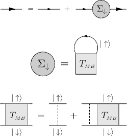
Figure 1: Ladder approximation for the self-energy. We restrict the analysis to the fluctuation part since the exchange part is important only in the case of magnetic ordering. Furthermore, we assume equal densities of spin-$\downarrow$ and spin-$\uparrow$ atoms, which makes the diagrams interchangeable with respect to spin-$\uparrow$ and spin-$\downarrow$.

After the analytic continuation $i\omega_{n}\rightarrow\omega+i0^{+}$, the retarded self-energy $\Sigma_{\downarrow}(\bm{q},\omega+i0^{+})$ can be computed from Eq. (2) using contour integration. Since the $T$-matrix may have poles away from the real axis, we cannot directly apply the spectral representation of the $T$-matrix to compute the self-energy. However, assuming that the $T$-matrix has poles either on the real axis or symmetrically with respect to the real axis, we arrive at a simple result for the imaginary part of the self-energy,

$$\text{Im}\,\Sigma_{\downarrow}(\bm{q},\omega)=\int \frac{\text{d}\bm{k}}{(2\pi)^{2}}\big{[}n_{B}(\omega+\varepsilon_{\bm{k}}-\mu)+n_{F}(\varepsilon_{\bm{k}}-\mu)\big{]}$$

$$\quad\times\,\text{Im}\,T_{\uparrow\downarrow}(\bm{q}+\bm{k},\omega+\varepsilon_{\bm{k}}-\mu),$$ (8)

where $n_{B}(\omega)$ denotes the Bose distribution. We have numerically verified that, for the parameter regime considered in this work, the $T$-matrix has poles at most on the real axis. The real part of the self-energy is calculated using the Kramers-Kronig relation

$$\text{Re}\,\Sigma_{\downarrow}(\bm{q},\omega)=\mathcal{P}\,\int_{-\infty}^{\infty}\frac{\text{d}z}{\pi}\,\frac{\text{Im}\,\Sigma_{\downarrow}(\bm{q},z)}{z-\omega},$$ (9)

where $\mathcal{P}$ denotes principal-value integration.

In 3D systems the appearance of poles in the $T$-matrix with a nonzero imaginary part is associated with the onset of the superfluid phase. This is the Thouless criterion Thouless (1960), and it can be used to identify the superfluid transition temperature $T_{c}$. In 2D Fermi gases, the superfluid transition takes place via the Berezinskii-Kosterlitz-Thouless (BKT) transition, which is not captured by our non-self-consistent $T$-matrix theory Loktev et al. (2001). In order to access the BKT physics, one needs to either consider the vertex corrections to the $T$-matrix formalism Loktev et al. (2001) or explicitly include phase fluctuations to a mean-field formalism Botelho and Sá de Melo (2006). Our non-self-consistent $T$-matrix theory should therefore be used at temperatures above $T_{c}$ where it provides a reasonable description of the system.

The retarded Green’s function is obtained by analytic continuation $G_{\downarrow}^{R}(\bm{q},\omega)=\mathcal{G}_{\downarrow}(\bm{q},i\omega_{n}\rightarrow\omega+i0^{+})$ from the thermal Green’s function given by the Dyson’s equation (1). The corresponding spectral function is defined as $A_{\downarrow}(\bm{q},\omega)=-2\,\text{Im}\,G_{\downarrow}^{R}(\bm{q},\omega)$, and it satisfies a sum rule $\int_{-\infty}^{\infty}\frac{\mathrm{d}\omega}{2\pi}\,A_{\downarrow}(\bm{q},\omega)=1$. We use this sum rule to verify the consistency of the numerical calculation. To obtain a physically correct spectral function for a strongly interacting initial gas of spin-$\uparrow$ and spin-$\downarrow$ atoms, the chemical potential $\mu$ has to be determined self-consistently. In the next section, we discuss the different self-consistent schemes for computing $\mu$.

II.2 Final state

In Ref. Zhang et al. (2012), the experimental findings were interpreted in terms of transitions between initial- and final-state polarons. In order to test this hypothesis, we consider the properties of the final-state atoms when they are dressed by the interactions with the initial state atoms. We take the interactions between atoms in hyperfine spin states $|\uparrow\rangle$ and $|f\rangle$ into account, using again the $T$-matrix formalism Schmidt et al. (2012). For the final-state atoms, the regularized polarization operator is given by

$$\chi_{0}^{\text{reg}} (\bm{q},i\Omega_{m})=$$

$$\int\frac{\mathrm{d}\bm{k}}{(2\pi)^{2}}\,\frac{n_{F}(\varepsilon_{\bm{k}+\bm{q}/2}-\mu)+n_{F}(\varepsilon_{\bm{k}-\bm{q}/2}+\Delta_{\uparrow f})}{i\Omega_{m}-2\varepsilon_{\bm{k}}-\frac{1}{2}\varepsilon_{\bm{q}}-\Delta_{\uparrow f}+\mu},$$ (10)

where $\Delta_{\uparrow f}$ is the level splitting between states $|\uparrow\rangle$ and $|f\rangle$. We have also denoted $\mu=\mu_{\downarrow}$. Since the final-state is initially empty, we have taken the final-state chemical potential to be $\mu_{f}=0$. We use the vacuum $T$-matrix to regularize the UV divergence. This introduces an additional interaction parameter $\varepsilon_{B}^{\prime}$ characterizing the final-state interactions.

Calculation of the dressed Green’s function is analogous to the polaron problem considered in Ref. Schmidt et al. (2012), and we obtain the self-energy $\Sigma_{f}$ by convoluting $\mathcal{G}_{0,\uparrow}$ with the many-body $T$-matrix $T_{\uparrow f}$. Since the $T$-matrix corresponding to the final-state interactions does not have poles away from the real axis Schmidt et al. (2012), we can directly apply spectral representation for the $T$-matrix and obtain Engelbrecht and Randeria (1992)

$$\text{Im}\,\Sigma_{f}(\bm{q},\omega)=\int \frac{\text{d}\bm{k}}{(2\pi)^{2}}\big{[}n_{B}(\omega+\varepsilon_{\bm{k}}-\mu)+n_{F}(\varepsilon_{\bm{k}}-\mu)\big{]}\,$$

$$\quad\times\,\text{Im}\,T_{\uparrow f}(\bm{q}+\bm{k},\omega+\varepsilon_{\bm{k}}-\mu).$$ (11)

Using Eq. (II.2), we calculate the real part using the Kramers-Kronig relation (9). In Ref. Schmidt et al. (2012), the self-energy of the final-state atoms was calculated at $T=0$ without invoking the Kramers-Kronig relation. As a check for the numerical calculation, we have verified that we reproduce the results of Ref. Schmidt et al. (2012) in the appropriate limit.

III Calculation of the chemical potential

In this section, we compare two different schemes for calculating the chemical potential of the initial-state atoms. The first one is the Noziéres–Schmitt-Rink (NSR) approximation Noziéres and Schmitt-Rink (1985); Schmitt-Rink et al. (1989); Tokumitu et al. (1993); Sá de Melo et al. (1993) and the second method is based on the number density given by the dressed Green’s function Serene (1989); Tsuchiya et al. (2009). The motivation for studying the two approximations is the fact that the NSR scheme is numerically much more affordable but expected to be accurate only when self-energy corrections are small Serene (1989). We are not aware of any explicit comparison of the two schemes for 2D systems.

Both aforesaid methods start from the thermodynamical potential $\Omega[\Sigma,\mathcal{G}]$ Serene (1989), where $\Sigma$ and $\mathcal{G}$ are self-energy and dressed Green’s function, respectively. The density is given by $n=-\frac{\partial\Omega}{\partial\mu}$, and the NSR approximation is obtained by replacing $\Omega[\Sigma,\mathcal{G}]\rightarrow\Omega[\Sigma,0]$. A more rigorous approximation suggested by Serene Serene (1989) corresponds to $\Omega[\Sigma,\mathcal{G}]\rightarrow\Omega[\Sigma,\mathcal{G}_{0}]$. The NSR approximation results in a number equation of the form Schmitt-Rink et al. (1989); Tokumitu et al. (1993); Serene (1989); Li and Yamada (2000)

$$n= 2\int\frac{\text{d}\bm{q}}{(2\pi)^{2}}\,n_{F}(\varepsilon_{\bm{q}}-\mu)+$$

$$\quad\quad\quad\frac{\partial}{\partial\mu}\int\frac{\text{d}\bm{q}}{(2\pi)^{2}}\,\mathcal{P}\int_{-\infty}^{+\infty}\frac{\mathrm{d}\omega}{\pi}\,n_{B}(\omega)\,\delta(\bm{q},\omega),$$ (12)

where $\delta(\bm{q},\omega)$ is the phase shift of the $T$-matrix, that is, $T_{\uparrow\downarrow}(\bm{q},\omega)=\big{|}T_{\uparrow\downarrow}(\bm{q},\omega)\big{|}\,e^{i\delta(\bm{q},\omega)}$. The total density can be written in terms of the Fermi energy as $n=m\varepsilon_{F}/\pi$. Numerical solution of Eq. (III) determines the chemical potential $\mu$ in terms of the Fermi energy $\varepsilon_{F}=k_{F}^{2}/2m$. We denote the temperature corresponding to Fermi energy by $T_{F}$.

A more rigorous alternative to the NSR number equation is a full number equation where the density is given by the dressed Green’s function Serene (1989); Perali et al. (2002); Tsuchiya et al. (2009)

$$n=\frac{2}{\beta}\sum_{i\omega_{n}}\int\frac{\text{d}\bm{q}}{(2\pi)^{2}}\,\mathcal{G}(\bm{q},i\omega_{n})\,e^{i\omega_{n}0^{+}},$$ (13)

such that $\mathcal{G}(\bm{q},i\omega_{n})$ is obtained from the Dyson’s equation (1). Using the spectral representation, we can cast Eq. (13) into

$$n=2\int\frac{\text{d}\bm{q}}{(2\pi)^{2}}\int_{-\infty}^{\infty}\frac{\mathrm{d}\omega}{2\pi}\,A(\bm{q},\omega)\,n_{F}(\omega).$$ (14)

The NSR number equation is obtained from Eq. (13) if $\mathcal{G}(\bm{q},i\omega_{n})$ is replaced with Serene (1989); Tsuchiya et al. (2009)

$$\mathcal{G}^{\text{NSR}}(\bm{q},i\omega_{n})=\mathcal{G}_{0}(\bm{q},i\omega_{n})+\mathcal{G}_{0}(\bm{q},i\omega_{n})\Sigma(\bm{q},i\omega_{n})\mathcal{G}_{0}(\bm{q},i\omega_{n}).$$ (15)

The NSR approximation is therefore formally reliable when corrections due to nonzero self-energy are small.

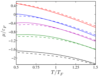
Figure 2: (Color online) Chemical potential as a function of temperature for different values of the interaction parameter $\eta$. From top to bottom: $\eta=1.5,\,0.5,\,0.25,\,0,$ and $-0.25$. The solid line corresponds to the full number equation [Eq. (14)] and the dashed line is the NSR approximation [Eq. (III)].

Before analyzing the 2D case, we note that in 3D (at the critical temperature), the NSR approximation and the full number equation yield chemical potentials that are almost identical Tsuchiya et al. (2009). In Fig. 2 we compare the results of the NSR approximation and the full number equation for a 2D Fermi gas. We present the results in terms of a dimensionless interaction parameter Feld et al. (2011); Schmidt et al. (2012),

$$\eta=-\frac{1}{2}\ln(\varepsilon_{B}/2\varepsilon_{F})=\ln(k_{F}a_{2D}).$$ (16)

The 2D unitarity is defined as $\eta=0$ since perturbative expansions in terms of $1/\eta$ diverge at this point Bloom (1975). A BCS-type superfluid and a Bose-Einstein condensate (BEC) of tightly bound molecules correspond to $\eta\gg 1$ and $\eta\ll-1$, respectively Randeria et al. (1989); Bertaina and Giorgini (2011). We observe that the difference between the NSR approximation and the full number equation is surprisingly small and the NSR theory is in fact a good approximation for the full number equation in the regime of parameters relevant to this work. As one would expect, the NSR approximation works best in the weakly interacting regime where $\eta>1$ (BCS limit). We will use, however, the chemical potential computed from the full number equation (14) in the subsequent calculations. In Fig. 3, we show the chemical potential as a function of the interaction parameter $\eta$ at different temperatures.

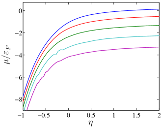
Figure 3: (Color online) Chemical potential at different temperatures as a function of the interaction parameter $\eta$. From top to bottom: $T/T_{F}=1.0,\,1.5,\,2.0,\,2.5,$ and $3.0$.

IV Spectral functions and quasiparticle spectrum

We consider two separate cases of strongly interacting Fermi atoms: (A) a balanced mixture of spin-$\downarrow$ and spin-$\uparrow$ atoms and (B) an impurity problem where an atom in a state $|f\rangle$ is immersed in a Fermi sea of spin-$\uparrow$ atoms. In the context of rf spectroscopy Sommer et al. (2012); Zhang et al. (2012), case (A) corresponds to the initial state of the system and case (B) describes the final-state atoms interacting with spin-$\uparrow$ atoms. In case (B) we assume that the impurity only interacts with spin-$\uparrow$ atoms since the rf pulse transferring atoms from state $|\downarrow\rangle$ to the final-state $|f\rangle$ simply rotates the atomic spin.

IV.1 Initial balanced mixture

The spectral function $A_{\downarrow}(\bm{k},\omega)$ for different values of the interaction parameter $\eta$ is shown in Fig. 4 for $T/T_{F}=0.5$ and $1.0$. In order to reach qualitative agreement with experimentally measured spectral functions Feld et al. (2011), one has to average the spectral function over the inhomogeneous density to account for the free atoms residing at the edge of the trap. Such atoms typically give rise to a peak at $\omega=-\mu$ He et al. (2005); Massignan et al. (2008); Chen and Levin (2009) (see also Sec. V.3). To understand the properties of the resulting rf spectra, we analyze next the different contributions to the quasiparticle spectra. For $\eta=-0.5$ and $0$, we find two distinct features in the spectral function: a broad incoherent band and a narrow coherent band. This two-band structure is a first indication of the pseudogap regime Perali et al. (2002); Stewart et al. (2008); Tsuchiya et al. (2009); Haussmann et al. (2009); Hu et al. (2010); Gaebler et al. (2010); Mueller (2011); Chien et al. (2010) since it suggests that removing a spin-$\downarrow$ particle from the system corresponds to creating and annihilating a pair of quasiparticles as in the usual BCS theory Tsuchiya et al. (2009).

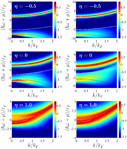
Figure 4: (Color online) Spectral function in the energy-momentum plane. Left panels: $T/T_{F}=0.5$. Right panels: $T/T_{F}=1.0$. The color scale is given by $\log_{10}A_{\downarrow}(\bm{k},\omega)$. For $\eta=-0.5$ and $\eta=0$, the dashed lines indicate a BCS-like dispersion given by Eq. (18) and the solid line is the threshold given by Eq. (17). For $\eta=1.0$, the dashed line corresponds to the free particle dispersion $\varepsilon_{\bm{k}}=\bm{k}^{2}/2m$ and the solid line indicates the dispersion of the attractive polaron.

We observe that the threshold for the incoherent branch in the spectral function (for $\eta=-0.5$ and $0$) is approximately given by

$$\omega_{\text{th}}(\bm{q})=\varepsilon_{\text{pair}}(\bm{q})+\mu,$$ (17)

where the bound-state energy $\varepsilon_{\text{pair}}(\bm{q})$ is given by the pole of the many-body $T$-matrix. We find that the poles have only a vanishingly small imaginary part. The threshold $\omega_{\text{th}}(\bm{q})$ is obtained from a simple argument: to create a spin-$\downarrow$ quasiparticle excitation with momentum $\bm{q}$, one can create a fermion pair with momentum $\bm{q}+\bm{k}$ and remove a spin-$\uparrow$ atom with momentum $\bm{k}$. This requires energy $E=\varepsilon_{\text{pair}}(\bm{k}+\bm{q})-(\varepsilon_{\bm{k}}-\mu_{\downarrow})$ and the threshold is obtained for $|\bm{k}|\simeq 0$. In a balanced system, this results in an energy threshold $\omega_{\text{th}}(\bm{q})=\varepsilon_{\text{pair}}(\bm{q})+\mu$ for the incoherent part of the quasiparticle spectrum. We note that a similar argument has been put forward earlier in Ref. Mueller (2011).

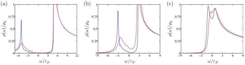
Figure 5: (Color online) Density of states $\rho(\omega)$ for (a) $\eta=-0.5$, (b) $\eta=0$, and (c) $\eta=1.0$. The upper (lower) curves with respect to the left peak correspond to $T/T_{F}=0.5$ ($T/T_{F}=1.0$). The density of states is measured in the units of density of states for an ideal Fermi gas, $\rho_{0}=m/\hbar^{2}$. The parameters are the same as in Fig. 4.

To gain more insight into the two branches of the spectral function for $\eta=-0.5$ and $0$, we fit a BCS-like dispersion Perali et al. (2002); Haussmann et al. (2009); Tsuchiya et al. (2009); Gaebler et al. (2010); Chien et al. (2010),

$$\varepsilon_{\text{BCS}}(\bm{k})=\sqrt{(\varepsilon_{\bm{k}}+U-\mu)^{2}+\Delta_{\text{pg}}^{2}},$$ (18)

to the numerical data. The pseudogap in Eq. (18) is denoted by $\Delta_{\text{pg}}$ and $U$ corresponds to a Hartree shift. The spectral function in Fig. 4 is shown relative to the chemical potential $\mu$ and therefore the two bands are described by an effective dispersion, $E_{\pm}(\bm{k})=\mu\pm\varepsilon_{\text{BCS}}(\bm{k})$ Haussmann et al. (2009); Chen and Levin (2009). The spectral function itself is peaked around the effective BCS-like dispersion given by $\varepsilon_{\pm}(\bm{k})=\pm\varepsilon_{\text{BCS}}(\bm{k})$. Results from a least squares fit are shown in Table 1 and we observe that the pseudogap $\Delta_{\text{pg}}$ decreases with increasing temperature and $\eta$. In general, we find that the coherent particle branch tends to be more accurately described by the BCS-like dispersion than the hole branch. From Fig. 4 and Table 1, we conclude that for $\eta=-0.5$ and $\eta=0$, the pseudogap regime extends at least up to $T=T_{F}$ if we define it to correspond to a regime where $\Delta_{\text{pg}}$ is nonzero. We note that the true pairing gap corresponding to the superfluid phase of a 2D Fermi gas has been calculated at $T=0$ in Ref. Bertaina and Giorgini (2011).

$\eta$	$T/T_{F}$	$\Delta_{\text{pg}}/\varepsilon_{F}$	$U/\varepsilon_{F}$
-0.5	0.5	3.90	0.08
-0.5	1.0	3.64	0.11
0	0.5	2.57	0.07
0	1.0	2.15	0.10

Table 1: Pseudogap $\Delta_{\text{pg}}$ and Hartree shift $U$ arising from a least-squares fit of a BCS-like dispersion to the numerical data in Fig. 4.

In the context of 3D Fermi gases, the pseudogap regime has been investigated by analyzing the density of states Tsuchiya et al. (2009); Mueller (2011). For 2D systems, the corresponding DOS is given by

$$\rho(\omega)=\int\frac{\mathrm{d}\bm{k}}{(2\pi)^{2}}\,A(\bm{k},\omega).$$ (19)

In Fig. 5, we show the DOS corresponding to Fig. 4. The density of states is measured with respect to the corresponding density of states of a noninteracting Fermi gas. In two spatial dimensions, ideal-gas DOS is a constant, $\rho_{0}=m/\hbar^{2}$. In terms of DOS, the pseudogap regime can be identified as a regime where DOS becomes strongly suppressed at zero energy (with respect to chemical potential) Tsuchiya et al. (2009); Mueller (2011). Using this criterion, we observe that the system is in the pseudogap regime for $\eta=-0.5$ and $\eta=0$ at least up to temperature $T=T_{F}$; see Fig. 5. On the other hand, the pseudogap practically vanishes for $\eta=1.0$ at $T/T_{F}=0.5$ and $1.0$. Another characteristic of the pseudogap regime is “backbending” of the quasiparticle dispersion in the single-particle spectral function near the Fermi wave vector $k_{F}$ Perali et al. (2011). From Fig. 4, we observe that the backbending near $k_{F}$ is clearly manifested in the spectral function for $\eta=-0.5$ and $\eta=0$ at $T/T_{F}=0.5$. We note that the backbending in the normal state of a Fermi gas has been discussed in Ref. Schneider and Randeria (2010), but in this case the backbending is expected to take place at $|\bm{k}|\gg k_{F}$. The BCS-like dispersion, suppression of DOS near zero energy, and backbending of the dispersion suggest that the gas is in the pseudogap regime for $\eta=-0.5$ and $\eta=0$ at least up to $T=T_{F}$.

For $\eta=1.0$, we find that the $T$-matrix does not have any poles (for $T/T_{F}=0.5$ and $1.0$) as the bound state is pushed against the two-particle continuum in the molecule spectral function. From Fig. 4, we observe that the spectral function (for $\eta=1.0$) at large momenta corresponds to free-particle-like excitations. The low-momentum part is more interesting since it is best described in terms of non-interacting polarons. In this regime ($|\bm{k}|<k_{F}$), the spectral weight is centered around energies that coincide with the dispersion of the attractive polaron. We define the (attractive) polaron energy as in Refs. Schmidt et al. (2012); Combescot et al. (2007); Massignan and Bruun (2011), that is, we consider a single spin-$\downarrow$ impurity embedded to a Fermi sea of spin-$\uparrow$ atoms. The polaron dispersion follows from equations

$$\omega(\bm{k})+\mu_{\downarrow}^{\prime}-\varepsilon_{\bm{k}}-\text{Re}\,\Sigma_{\downarrow}\big{(}\bm{k},\omega(\bm{k})\big{)}=0,$$ (20)

$$\omega_{p}(\bm{k})=\omega(\bm{k})+\mu_{\downarrow}^{\prime},$$ (21)

where $\mu_{\downarrow}^{\prime}$ is tuned such that state $|\downarrow\rangle$ is empty. To ensure that the calculation is self-consistent, we set $\mu_{\uparrow}=\mu$, where $\mu$ is solved from the number equation (14) corresponding to the original balanced system. Equations (20) and (21) generalize the zero-temperature analysis Schmidt et al. (2012) to finite temperatures. Moreover, at $T=0$, Eqs. (20) and (21) are equivalent to the analysis based on a variational wave function for the polaron Zöllner et al. (2011); Parish (2011).

Our analysis suggests that outside the pseudogap regime, even a balanced 2D Fermi gas can be effectively described as a gas of noninteracting polarons. For 2D systems, the polaron description has been used by Zhang et al. Zhang et al. (2012) as a possible explanation for their experimental observations. For 3D systems, similar speculations have appeared earlier in Ref. Schirotzek et al. (2009). Our findings thus support the scenario put forward in Ref. Zhang et al. (2012) and indicate a crossover (at fixed temperature) from a polaron gas for small attraction to a pseudogap regime at strong attraction.

IV.2 Final state – impurity

The quasiparticle excitations of the final state have been thoroughly discussed in Ref. Schmidt et al. (2012) at $T=0$. The main features in the final-state spectral function correspond to the attractive and the repulsive polaron Massignan and Bruun (2011); Schmidt et al. (2012); Schmidt and Enss (2011), while the contribution from a bound state carries only a small spectral weight. Here we briefly discuss the qualitative changes that the finite temperature induces. As in Ref. Schmidt et al. (2012), we first assume that the initial mixture of spin-$\uparrow$ and spin-$\downarrow$ atoms is noninteracting. The chemical potential is then given by the ideal gas expression $\mu_{0}(T)=k_{B}T\,\ln\big{(}e^{\varepsilon_{F}/k_{B}T}-1\big{)}$. The finite temperature results in two qualitative changes: the attractive polaron acquires a finite lifetime and the molecule-hole continuum merges with the attractive polaron branch. Furthermore, as the temperature increases, the spectral weight is distributed more equally between attractive and repulsive polarons. We note that the properties of 2D polarons have recently been studied experimentally in Refs. Fröhlich et al. (2011); Koschorreck et al. (2012) and the experimental data agrees reasonably well with the non-self-consistent $T$-matrix calculation Schmidt et al. (2012); Koschorreck et al. (2012).

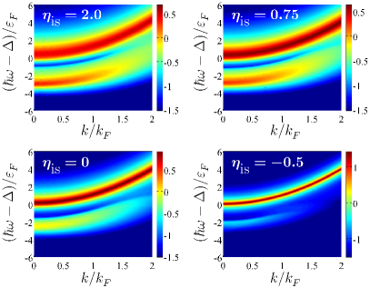
Figure 6: (Color online) Spectral function of the final-state atom (impurity) when the majority atoms are dressed by strong initial-state interactions. The color scale corresponds to $\log_{10}A_{f}(\bm{k},\omega)$. The strength of the initial-state interaction is denoted by $\eta_{\text{is}}$ in the figure. The temperature is set to $T=T_{F}$ and interactions between the final-state atom and spin-$\uparrow$ atoms correspond to $\eta_{\text{fs}}=0$. The level splitting between states $|\uparrow\rangle$ and $|f\rangle$ is denoted by $\Delta$ and is assumed to be positive.

Next we consider the case where the impurity (final-state atom) is dynamically created from an interacting, balanced gas of spin-$\uparrow$ and spin-$\downarrow$ atoms. The chemical potential is now determined by the interacting initial state and it is solved from the number equation (14). In Fig. 6, we show the spectral function of the final state atoms for different initial-state interactions. For illustrative purposes, we fix the final-state interaction to $\eta_{\text{fs}}=0$. In contrast to the experiments in Refs. Sommer et al. (2012); Zhang et al. (2012), this final-state interaction is in the strongly interacting regime. With increasing initial-state attraction, the initial state becomes increasingly paired, and the added impurity is less likely to distort the cloud of majority atoms. Thus the impurity behaves more and more like a free particle as one approaches the BEC limit. In Fig. 6, this is manifested as a suppression of the spectral weight associated with the polaron states.

V Radio-frequency spectroscopy

We consider radio-frequency spectroscopy in which a balanced mixture of atoms in hyperfine states $|i_{1}\rangle\equiv|\uparrow\rangle$
and $|i_{2}\rangle\equiv|\downarrow\rangle$ is coupled to rf photons inducing a transition $|\downarrow\rangle\rightarrow|f\rangle$ Chen et al. (2009). Within the linear response framework, one obtains

$$I_{\mathrm{rf}}(\omega_{\mathrm{rf}})=-\pi\Omega_{\mathrm{rf}}^{2}\,\text{Im}\,\chi_{R}(\bm{k}=0,-\omega_{\mathrm{rf}}-\mu_{\downarrow}+\mu_{f}).$$ (22)

At finite temperatures, the retarded correlation function $\chi_{R}$ can be computed from the corresponding time-ordered correlation function as Doniach and Sondheimer (1974)

$$\text{Im}\,\chi_{R}(\bm{k},\omega)=\tanh(\frac{1}{2}\beta\omega)\,\text{Im}\,\chi(\bm{k},\omega),$$ (23)

where

$$\chi(\bm{r}-\bm{r}^{\prime},t-t^{\prime})=$$

$$-i\theta(t-t^{\prime})\langle[\psi_{f}^{\dagger}(\bm{r},t)\psi_{\downarrow}(\bm{r},t),\psi_{\downarrow}^{\dagger}(\bm{r}^{\prime},t^{\prime})\psi_{f}(\bm{r}^{\prime},t^{\prime})]\rangle.$$ (24)

Since we evaluate the correlation function for $\omega=-\omega_{\mathrm{rf}}-\mu+\mu_{f}\ll-\varepsilon_{F}$, we have $\tanh(\frac{1}{2}\beta\omega)\approx-1$. We neglect the vertex corrections Perali et al. (2008); Pieri et al. (2009, 2011) and obtain

$$\chi(\bm{k}= 0,i\Omega_{n})=$$

$$\frac{1}{\beta}\sum_{i\omega_{m}}\int\frac{\mathrm{d}\bm{q}}{(2\pi)^{2}}\mathcal{G}_{f}(\bm{q},i\omega_{m})\mathcal{G}_{\downarrow}(\bm{q},i\Omega_{n}+i\omega_{m}).$$ (25)

Using the spectral representation for the Green’s functions, the analytic continuation can be performed exactly and we obtain

$$I_{\mathrm{rf}}(\omega)= \frac{\pi}{2}|\Omega_{\mathrm{rf}}|^{2}\int\frac{\mathrm{d}\bm{q}}{(2\pi)^{2}}\int\frac{\mathrm{d}z}{2\pi}\,A_{\downarrow}(\bm{q},z-\omega-\Delta_{\uparrow f}-\mu_{\downarrow})$$

$$\times A_{f}(\bm{q},z)\big{[}n_{F}(z-\omega-\Delta_{\uparrow f}-\mu_{\downarrow})-n_{F}(z)\big{]},$$ (26)

where $\Delta_{\uparrow f}$ is the level splitting between states $|\downarrow\rangle$ and $|f\rangle$ and we have defined the detuning $\omega=\omega_{\mathrm{rf}}-\Delta_{\uparrow f}$. If interactions between states $|\uparrow\rangle$ and $|f\rangle$ are negligible, then the final-state spectral function becomes $A_{f}(\bm{q},z)=2\pi\delta(z-\varepsilon_{\bm{q}}-\Delta_{\uparrow f})$. Here we have set $\mu_{f}=0$ since the final state is initially empty. We have also taken explicitly into account the level splitting $\Delta_{\uparrow f}$. The rf current takes the form

$$I_{\mathrm{rf}}(\omega)=\frac{\pi|\Omega_{\mathrm{rf}}|^{2}}{2}\int\frac{\mathrm{d}\bm{q}}{(2\pi)^{2}}\,A_{\downarrow}(\bm{q},\varepsilon_{\bm{q}}-\mu_{\downarrow}-\omega)\,n_{F}(\varepsilon_{\bm{q}}-\mu_{\downarrow}-\omega),$$ (27)

where we have neglected the term $n_{F}(\varepsilon_{\bm{q}}+\Delta_{\uparrow f})$ corresponding to the occupation of the final state. At finite temperatures this term is, in principle, nonzero but we assume $\Delta_{\uparrow f}\gg\varepsilon_{F}$, which renders $n_{F}(\varepsilon_{\bm{q}}+\Delta_{\uparrow f})$ negligible. In the current experiments Zhang et al. (2012); Sommer et al. (2012), the Zeeman splitting between the relevant hyperfine spin states is $\Delta_{\uparrow f}\sim 50$ MHz Bartenstein et al. (2005), whereas the Fermi energy is in the range $\varepsilon_{F}\sim 10-250$ kHz Zhang et al. (2012); Sommer et al. (2012). Hence, we expect that neglecting the occupation of the final state is justified even at temperatures $T\sim T_{F}$.

We note that the more general form of the rf current in Eq. (V) is phenomenological since all vertex corrections are excluded. Therefore our formalism does not include bound-to-bound transitions Schunck et al. (2008); Pieri et al. (2009). Since Eq. (V) contains information about the final-state polarons, we will use it to analyze the NCSU experiment.

V.1 Quasi-2D geometry and experimental parameters

To compare our results to the experiments Sommer et al. (2012); Zhang et al. (2012), we need to establish a connection between the dimensionless interaction parameter $\eta$ and an external magnetic field $B$ which is used to tune the interactions via the Feshbach resonance. Since the experiments are performed in a quasi-2D geometry, we calculate the two-body binding energy $\varepsilon_{B}$ in terms of the 3D scattering length $a_{3D}$ using the quasi-2D form of the $T$-matrix Petrov and Shlyapnikov (2001); Bloch et al. (2008); Pietilä et al. (2012),

$$\mathcal{T}_{0}(\omega)=\frac{2\sqrt{2\pi}/m}{\ell_{z}/a_{3D}-\mathcal{F}(-\omega/\omega_{z})},$$ (28)

where function $\mathcal{F}(z)$ is given by

$$\mathcal{F}(z)=\int_{0}^{\infty}\,\frac{\mathrm{d}u}{\sqrt{4\pi}}\,\frac{1}{u^{3/2}}\bigg{(}1-\frac{e^{-zu}}{\sqrt{\frac{1}{2u}(1-e^{-2u})}}\bigg{)}.$$ (29)

The trap frequency along the tightly confined direction is denoted by $\omega_{z}$ and the length scale associated with the confinement is given by $\ell_{z}=\sqrt{1/m\omega_{z}}$ for atoms with mass $m$. The two-body binding energy $\varepsilon_{B}$ corresponds to a pole of the vacuum $T$-matrix and is determined by the equation (we assume $\varepsilon_{B}>0$)

$$\ell_{z}/a_{3D}-\mathcal{F}(\varepsilon_{B}/\omega_{z})=0.$$ (30)

We solve Eq. (30) numerically to obtain $\varepsilon_{B}=\varepsilon_{B}(\ell_{z}/a_{3D})$. To convert the external magnetic field to the 3D scattering length $a_{3D}$, we use the parameters of Ref. Bartenstein et al. (2005). The two-body binding energy is converted to the dimensionless interaction parameter $\eta$ using Eq. (16).

V.2 MIT experiment Sommer et al. (2012)

The MIT experiment Sommer et al. (2012) is performed using the three lowest sublevels $|1\rangle$, $|2\rangle$, and $|3\rangle$ on the ⁶Li ground-state manifold Bartenstein et al. (2005). The set of initial states is given by $\{|\uparrow\rangle,|\downarrow\rangle\}=\{|1\rangle,|3\rangle\}$, and the final state corresponds to $|f\rangle=|2\rangle$. Interactions between atoms in the two initial states are enhanced by a Feshbach resonance at $B=690.4$ G. The initial state $|\downarrow\rangle$ coupled with the final state $|f\rangle$ is chosen such that the final-state interactions are minimized Sommer et al. (2012). In the MIT experiment, the two-body binding energy of the final state dimer is much larger than the initial-state dimer energy, $\varepsilon_{B}^{\prime}\gg\varepsilon_{B}$. As in the 3D case Schunck et al. (2008), the final-state interactions are important only if $\eta_{\uparrow f}$ corresponding to $\varepsilon_{B}^{\prime}$ is close to the 2D unitarity $\eta=0$. The MIT experiment is outside this regime and hence we neglect the final-state interactions altogether. We note that the final-state interactions are important for the bound-to-bound transition in the rf spectrum Langmack et al. (2012), but we do not consider this transition in the present work. Although the MIT experiment studied the whole dimensional crossover from 3D to 2D, we concentrate on the 2D limit of the experiment. Using the methods of Ref. Pietilä et al. (2012), it is possible to study rf spectroscopy across the whole dimensional crossover. Due to the multiple bands involved with this formalism, the calculation becomes numerically more demanding and we postpone such studies for future research.

B [G]	$\eta_{\uparrow\downarrow}$
690.7	-0.504
720.7	-0.364

Table 2: Interaction parameter $\eta$ corresponding to the 2D limit of the MIT experiment. The values of the experimental parameters can be found from Ref. Sommer et al. (2012). To convert the external magnetic field to the 3D scattering length $a_{3D}$, we have used the parameters from Ref. Bartenstein et al. (2005).

The dimensionless interaction parameter $\eta$ for the initial-state interactions is shown in Table 2 for the relevant values of the external magnetic field. The temperature at the MIT experiment was estimated to be of the order of $T_{F}$ and the peak Fermi energy was approximately $\varepsilon_{F}=h\times 10$ kHz Sommer et al. (2012). We note that the data corresponding to the deepest optical lattice (the regime of our interest) was deeply in the 2D regime since $\varepsilon_{F}/\hbar\omega_{z}\approx 0.04$. Thus we expect that this limit is well described by our 2D calculation.

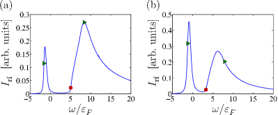
Figure 7: (Color online) Radio-frequency spectra corresponding to the MIT experiment Sommer et al. (2012). The external magnetic field is (a) $B=690.7$ G and (b) $B=720.7$ G. The dimensionless interaction parameter $\eta$ for the initial-state interactions is given in Table 2. The temperature is (a) $T/T_{F}=1.5$ and (b) $T/T_{F}=2.0$. The dots indicate the threshold given by Eq. (31) and the triangles arise from the BCS-like dispersion at zero momentum; see Eqs. (18) and (32).

Since the final-state interactions mainly affect the tails of the rf spectra and round off the onset of the pairing peak Sommer et al. (2012); Langmack et al. (2012), the qualitative features of the rf spectra measured in Ref. Sommer et al. (2012) can be understood by studying the spectral function of the initial state. In the absence of final-state interactions, Eq. (27) suggests that the broad peak (“pairing peak”) at positive detuning arises from the incoherent part of the spectral function corresponding to the dissociation of the preformed pairs (see Fig. 4). In Sec. IV.1 we showed that the threshold for the incoherent part is approximately given by $\omega_{\text{th}}(\bm{q})=\varepsilon_{\text{pair}}(\bm{q})+\mu$. Using Eq. (27) we obtain a threshold

$$\omega_{0}=-\omega_{\text{th}}(\bm{q}=0)-\mu=-\varepsilon_{\text{pair}}(\bm{q}=0)-2\mu.$$ (31)

Thus the onset of the pairing peak is related to the binding energy of the paired fermions. From Fig. 7, we observe that the onset of the incoherent peak is indeed given quite accurately by $\omega_{0}$.

In the pseudogap regime, the spectral function is peaked around an effective BCS-like dispersion and Eq. (27) can be used to find the corresponding frequencies in the rf spectrum,

$$\omega_{\pm}(\bm{q})=\varepsilon_{\bm{q}}\pm\varepsilon_{\text{BCS}}(\bm{q})-\mu.$$ (32)

However, evaluating $\omega_{\pm}(\bm{q})$ at $\bm{q}=0$ does not directly give the peak location since the spectral function is integrated over momentum; see Fig. 7. Furthermore, we note that the quasiparticle dispersion starts to deviate from the BCS form for $T/T_{F}=2.0$ in Fig. 7(b).

The experimentally measured binding energies (the onset of the pairing peak) were found to agree reasonably well with the energies of the two-body bound states in quasi-2D systems Sommer et al. (2012); Orso et al. (2005). Our calculation for the chemical potential at the regime of the MIT experiment ($T\gtrsim T_{F}$ and $\eta<0$) predicts $\mu$ to be large and negative. Hence, the polarization operator $\chi_{0}^{\text{reg}}(\bm{q},\omega)$ in Eq. (II.1) gives a negligible contribution to the many-body $T$-matrix. In this limit, the poles of the $T$-matrix can be solved exactly and we obtain $\varepsilon_{\text{pair}}(\bm{q})=-\varepsilon_{B}-2\mu+\frac{1}{2}\varepsilon_{\bm{q}}$. The onset of the pairing peak becomes $\omega_{0}(\bm{q})=\varepsilon_{B}-\frac{1}{2}\varepsilon_{\bm{q}}$, which explains why the experiment is in good agreement with the two-body calculation. In order to observe many-body effects, one should either consider lower temperatures or quench the system rapidly to the strongly interacting regime as suggested in Ref. Pietilä et al. (2012).

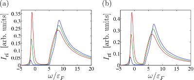
Figure 8: (Color online) Radio-frequency spectrum at different temperatures corresponding to the 2D limit of Ref. Sommer et al. (2012). The external magnetic field is (a) $B=690.7$ G and (b) $B=720.7$ G. The dimensionless interaction parameter $\eta$ for the initial-state interactions is shown in Table 2. The temperatures are given by $T/T_{F}=1.0,1.5,$ and $2.0$ (from top to bottom with respect to the peak on the right-hand side) in both panels.

To probe the temperature dependence of the rf spectra, we show the calculated rf current at different temperatures in Fig. 8. We find the best qualitative agreement with Ref. Sommer et al. (2012) for temperatures $T/T_{F}\simeq 1.5$ at the Feshbach resonance ($B=690.7$ G) and $T/T_{F}\simeq 2.0$ on the BCS side of the resonance ($B=720.7$ G). To reach a quantitative agreement with the experimental data, the rf signal needs to be averaged over the inhomogeneous density. Furthermore, one has to use the temperature and the Fermi energy as fitting parameters since they were not exactly known in Ref. Sommer et al. (2012).

Since the spectral weight carried by the coherent branch of the spectral function increases with increasing temperature (see Fig. 4), the corresponding peak in the rf spectrum at negative detuning becomes stronger with increasing temperature (Fig. 8). Within our theory, this peak arises from thermally excited quasiparticles and corresponds to unpaired atoms. For the fairly high temperatures required to obtain a qualitative agreement with the MIT data, the depletion in the density of states is qualitatively the same as in Fig. 5(a). The gas is therefore at the crossover region between the pseudogap regime and the regime of a normal gas of bosonic molecules Watanabe et al. (2010).

V.3 NCSU experiment Zhang et al. (2012)

In contrast to the MIT experiment, the NCSU experiment found resonances in the rf spectrum that do not correspond to paired fermions but transitions between polaronic states. Our analysis in Sec. IV.1 suggests that a balanced gas (the initial state) in the weakly attractive regime can be considered as a gas of noninteracting polarons. Since the atoms in the final state can be described in terms of polarons (see Sec. IV.2), the experimental picture of transitions between polaronic states arises naturally.

B [G]	$\eta_{\uparrow\downarrow}$	$\eta_{\downarrow f}$
719	-0.330	1.626
810	0.967	1.767

Table 3: Dimensionless interaction parameters corresponding to the NCSU experiment Zhang et al. (2012). initial-state interactions are denoted by $\eta_{\uparrow\downarrow}$, and $\eta_{\downarrow f}$ corresponds to the final-state interactions. For other magnetic fields and trap depths considered in Ref. Zhang et al. (2012), the initial- and the final-state interactions are similar and give qualitatively the same results.

We first analyze the line shape of the rf spectrum in a homogeneous system for the parameters of the NCSU experiment. The dimensionless parameters $\eta_{\uparrow\downarrow}$ and $\eta_{\uparrow f}$ characterizing the initial- and final-state interactions are shown in Table 3. We use the values reported in Ref. Zhang et al. (2012) for the initial and the final-state dimer energies and determine the interaction parameter $\eta$ using Eq. (16). Since the final-state interactions are weak, we expect that our phenomenological model in Eq. (V) is a good description of the dressed final-state atoms.

The rf spectra corresponding to the parameters of Table 3 are shown in Fig. 9. For strong attraction [Fig. 9(a)], the pairing peak at positive detuning $\omega$ is again characterized by the threshold frequency $\omega_{0}$ given by Eq. (31). The sharp peak around zero detuning arises from the unpaired atoms as in the MIT experiment. We find that the inclusion of the final-state interactions tends to lower the peak corresponding to the unpaired atoms. A crucial difference between Figs. 9(a) and (b) is the absence of a pole in the $T$-matrix for the parameters of Fig. 9(b). Since most of the data presented in Ref. Zhang et al. (2012) fall to the same regime of initial- and final-state interactions as Fig. 9 (b), the measured rf spectra cannot be explained in terms of confinement-induced molecules.

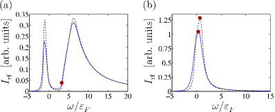
Figure 9: (Color online) Radio-frequency spectrum corresponding to the NCSU experiment Zhang et al. (2012) for (a) $B=719$ G and (b) $B=810$ G (solid lines). The dimensionless interaction parameters for the initial- and the final-state interactions are shown in Table 3. The temperature is $T/T_{F}=1.5$ in both panels. The dashed line denotes the rf spectrum in the absence of final state interactions. In panel (a), the dot indicates the threshold given by Eq. (31), and in panel (b), the dots correspond to the polaron threshold; see the main text. The single peak structure in panel (b) persists down to $T/T_{F}=0.5$, which is the lowest temperature considered in this work.

Based on the analysis in Sec. IV.1, we argue that the origin of the single peak in Fig. 9(b) is related to the effective description of the gas in terms of noninteracting polarons. In the absence of final state interactions, we expect the location of the peak to be given by $\omega_{0}=-\omega_{p}^{\text{(is)}}(\bm{k}=0)$, where $\omega_{p}^{\text{(is)}}(\bm{k})$ is the initial-state polaron energy given by Eq. (21). Furthermore, when the final-state interactions are included, the free-particle dispersion of the final-state atoms is effectively replaced by the final-state polaron dispersion, and we obtain an estimate for the peak location: $\omega_{0}^{\prime}=-\omega_{p}^{\text{(is)}}(\bm{k}=0)+\omega_{p}^{\text{(fs)}}(\bm{k}=0)$, where $\omega_{p}^{\text{(fs)}}(\bm{k}=0)$ is the energy of the final-state polaron. From Fig. 9 (b), we observe that the estimates $\omega_{0}$ and $\omega_{0}^{\prime}$ are indeed quite accurate.

Similarly to the MIT experiment Sommer et al. (2012), the NCSU experiment has a dual peak structure in the measured rf spectra Zhang et al. (2012). Since our calculation for a homogeneous system predicts only a single peak, we argue that the second peak is due to the averaging of the rf signal over an inhomogeneous density. As in 3D systems He et al. (2005); Massignan et al. (2008); Chen and Levin (2009), the auxiliary peak arises from unpaired atoms in the low-density region at the edge of the trap. To show this explicitly, we average the rf signal over the inhomogeneous density using the local density approximation (LDA) Chiofalo et al. (2002). Within the LDA, the local chemical potential is given by $\mu(\bm{r})=\mu-\frac{1}{2}m\omega_{\perp}^{2}r^{2}$. The local density $n_{\text{LDA}}(\bm{r})$ is calculated using the number equation (14) and the density averaged rf signal is obtained as $I_{\text{rf}}^{\text{LDA}}(\omega)=\int\text{d}\bm{r}\,n_{\text{LDA}}(\bm{r})I_{\text{rf}}(\omega,\bm{r})$, where $I_{\text{rf}}(\omega,\bm{r})$ is the rf signal given by Eq. (V) for the local chemical potential $\mu(\bm{r})$.

Rather than attempting to exactly reproduce the experimentally measured lineshapes, we use the LDA to confirm that the auxiliary peak in the rf spectrum near the zero detuning is due to trap average. To this end, we fix the initial- and the final-state interaction strengths to the values given in Table 3 and take the Fermi energy $\varepsilon_{F}=\omega_{\perp}\sqrt{N_{\text{tot}}}$ to be $114.5$ kHz; see Ref. Zhang et al. (2012). The total number of atoms is given by $N_{\text{tot}}=\int\text{d}\bm{r}\,n_{\text{LDA}}(\bm{r})$ and the peak value of the chemical potential can be tuned to reach a desired number of atoms Massignan et al. (2008); Chiofalo et al. (2002). In Fig. 10, we show the rf current for different numbers of atoms. We implicitly assume that the trap frequency is tuned such that $\varepsilon_{F}$ remains constant.

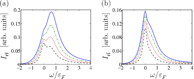
Figure 10: (Color online) Trap-averaged rf signal corresponding to (a) $T/T_{F}=0.5$ and (b) $T/T_{F}=1.0$. The dimensionless interaction parameters are $\eta_{\uparrow\downarrow}=0.967$ and $\eta_{\downarrow f}=1.767$. The rf current is scaled by the total number of particles which is given by (a) $N_{\text{tot}}=2234,1791,1476,1214$, and (b) $N_{\text{tot}}=2073,1810,1494,1190$ (from top to bottom).

On a qualitative level, our theoretical calculation agrees with the picture put forward in Ref. Zhang et al. (2012): in the regime of the experimental parameters, the rf spectrum is best described in terms of transitions between noninteracting polaronic states. In general, we find that the location of the right-hand side peak in the trap-averaged rf signal [Fig. 10 (a)] is not directly related to the polaron energy corresponding to the peak chemical potential. Therefore, locally resolved rf spectroscopy Schirotzek et al. (2008) is desirable to confirm the polaron picture. Within the appropriate temperature range, our LDA calculation qualitatively reproduces the double-peak structure observed in the experiment; see Fig. 10(a). The auxiliary peak due to the trap average becomes more pronounced at high temperatures and renders the polaron peak indistinguishable if the total number of atoms is too small [Fig. 10(b)].

VI Discussion

In this work, we analyzed pairing in two-dimensional Fermi gases above the superfluid transition temperature. For a gas composed of an equal number of spin-$\uparrow$ and spin-$\downarrow$ fermions, we found evidence of a crossover from a noninteracting gas of polarons to a pseudogap regime characterized by a BCS-like dispersion and reduced single-particle density of states near the Fermi energy. The details of this crossover as well as the properties of the effective polarons in a balanced Fermi gas clearly call for further investigations.

We also analyzed two recent experiments that performed radio-frequency spectroscopy for 2D Fermi gases Sommer et al. (2012); Zhang et al. (2012). To take into account the polaronic properties of the final-state atoms, we introduced a phenomenological model that uses dressed Green’s functions for both initial- and final-state atoms in the calculation of the rf spectrum. Although this approach does not include the vertex corrections Perali et al. (2008); Pieri et al. (2009, 2011), our model qualitatively explains the different observations in Refs. Sommer et al. (2012); Zhang et al. (2012). In particular, our polaron-to-pseudogap crossover can be used to explain the apparent dichotomy in Refs. Sommer et al. (2012); Zhang et al. (2012). Our calculations suggest that Ref. Sommer et al. (2012) probed the pseudogap regime, while Ref. Zhang et al. (2012) provided data from the polaron side of the crossover.

In Ref. Sommer et al. (2012), the measured binding energies were found to be close to the energies of the corresponding two-body bound states. We demonstrated that this effect arises at the high-temperature regime, where many-body contributions to the experimentally measured thresholds in the rf spectrum become negligibly small. In order to clearly see the effect of many-body corrections to the measured binding energies, the temperature should be lower or the system should be quickly quenched to the strongly interacting regime as suggested in Ref. Pietilä et al. (2012).

Another interesting and theoretically largely unexplored direction is the dimensional crossover from 2D to 3D. In Ref. Sommer et al. (2012), the dimensional crossover was explicitly probed, and in Ref. Zhang et al. (2012), implications of the quasi-2D nature of the gas seem to be unavoidable since the Fermi energy was larger than the level splitting in the tightly confined direction. The formalism constructed for molecule formation in quasi-2D systems Pietilä et al. (2012) has recently been extended to study the polaron problem Levinsen and Baur and could be used to investigate the rf spectroscopy of quasi-2D systems.

Note added in proof: Recently, two preprints discussing the pseudogap phase in 2D Fermi gases have appeared Klimin et al. ; Watanabe et al. .