A new approach to the optimization of the extraction of astrometric and photometric information from multi-wavelength images in cosmological fields.

Abstract

This paper describes a new approach to the optimization of information extraction in multi-wavelength image cubes of cosmological fields.
The objective is to create a framework for the automatic identification and tagging of sources according to various criteria (isolated source, partially overlapped, fully overlapped, cross-matched, etc) and to set the basis for the automatic production of the SEDs (spectral energy distributions) for all objects detected in the many multi-wavelength images in cosmological fields.
In order to do so, a processing pipeline is designed that combines Voronoi tessellation, Bayesian cross-matching, and active contours to create a graph-based representation of the cross-match probabilities. This pipeline produces a set of SEDs with quality tags suitable for the application of already-proven data mining methods.
The pipeline briefly described here is also applicable to other astrophysical scenarios such as star forming regions.

1 Introduction

Single-field multi-wavelength studies obtained with very heterogeneous instruments and telescopes are very common nowadays. Deep cosmological surveys are extreme examples of such studies that combine photometric data from the $\gamma$-rays to the radio-wavelengths, offering complementary yet astonishingly different views of the same extragalactic objects. These image cubes carry both astrometric and photometric information of tens of thousands of sources, which bring their analysis into the realm of statistics and data mining.

One of the key aspects of the systematic analysis of these image cubes is the reliability of the scientific products derived from them. In this work, we concentrate on the generation of spectral energy distributions (SEDs) of extragalactic sources in deep cosmological fields. The techniques outlined here are nevertheless of much wider application in other astrophysical scenarios. We concentrate in particular in the problem of tagging the quality of a derived SED from the perspective of the underlying cross-match decisions.

In Section 2 we describe the project and its aims, and the techniques utilized to derive spectral energy distributions from deep cosmological image cubes; Section 3 briefly summarizes the Bayesian approach that serves as the basis for the developments presented in Section 4 which introduces the possibility of non-detections in the Bayesian formalism. Finally, Section 5 describes the results obtained for the application of the extended formalism to a toy problem, and Section 6 summarizes the main conclusions.

2 Deep cosmological fields: the analysis pipeline

In this work we address the problem of deriving spectral energy distributions and the labelling of the different sources detected in multi-wavelength deep images of cosmological fields. Is is compounded of several sub-tasks, such as the cross-matching of the sources detected in individual images, the tagging of potential overlaps and the derivation of optimal regions for sky subtraction.

Images of the same field obtained with different spatial resolutions, sensitivities and in various wavelengths will offer complementary views of the same sources, but also views that can be inconsistent if we do not take into account all these factors. Let us take for example the case where a galaxy A detected in low resolution infrared bands has a flux density below the detection threshold of a mid-infrarred survey, and has several potential counterparts in visible wavelengths, many of which do not actually correspond to galaxy A, but to galaxies close to the line of sight. In addition to this, let us consider the possibility where one of the visible counterparts (but not the source that corresponds to galaxy A) is actually detected in the mid-infrared image. A sound cross-matching approach must necessarily address this problem in a probabilistic manner, including a requirement on astrometric and photometric consistency. The approach that we propose here is based on a Bayesian formalism of the problem of cross-matching catalogues that, as a by-product produces a quantitative measure of the validity of the counterpart assignment and flags SEDs that may be affected by source overlapping within and across images taken in several bands.

In the first stage of our analysis pipeline, the catalogue extraction tool Sextractor Astron.Astrophys.Suppl.Ser:117.393-404 is applied to each image separately. The catalogue thus obtained (including astrometric and photometric information) is used as the basis for a 2D Voronoi (Delaunay) tessellation of the images that defines a polygon in the corresponding coordinates (e.g., celestial, pixel) for each source.

This 2D Voronoi tessellation of the images provides us with a preliminary categorization of sources into the candidate categories of isolated source and partially or totally contaminated by neighbouring sources. A source is labelled as candidate for isolated source if it is fully contained in its Voronoi cell and none of the sources from the Voronoi cells surrounding the source under consideration is contaminating it. In this initial stage, the source extension is defined by its Kron ellipse Astron.Astrophys.Suppl.Ser:117.393-404 although subsequent refinements can be applied with more refined contours (active contours for example). This labelling procedure only considers information from one single image. The definition can be extended by defining an isolated source as one which is i) isolated in the lowest resolution image; ii) only has one counterpart in the projection of its Voronoi cell in all other images and, iii) each of these counterpars is also isolated in the sense defined above.

Figure 1 shows an example of the result of the implementation of this preliminary labelling process to the Hubble Deep Field image taken by the IRAC instrument on channel $3.6\mu m$.

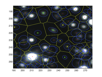
Figure 1: Examples of isolated and partially contaminated sources in the Hubble Deep Field image of IRAC instrument on channel $3.6\mu m$.

A simple improvement of this approach consists in taking into account the source morphology in the determination of the isolation cell by applying Support Vector Machines for the determination of the maximum margin hyperplanes separating sources.

The result from the previous steps will produce a set of two-dimensional vectors, $\vec{x_{ij}}$ ,which represent the celestial coordinates of the source $j$ in catalogue $i$ together with the preliminary labelling described in the previous paragraphs. From this set of vectors, we aim at constructing reliable SEDs by cross-matching them taking into account the astrometric information, the photometric information and the instrument sensitivities. In the following, we will summarize the Bayesian formalism developed in APJ.679:301-309 that we further extend to potential non-detections.

3 Cross-Matching of multi-wavelength astronomical sources

The work presented in APJ.679:301-309 , and summarized in the following paragraphs, proposes a bayesian approach for the decision-making problem of defining counterparts in multi-band image cubes.

Let us define $M$ as the hypothesis that the position of a source is on the celestial sphere, and let us parametrize this position in terms of a three-dimensional normal vector $\vec{m}$. Let us assume that we have $n$ overlapping images of a given field, and let us call data $D=\{\vec{x_{1}},\vec{x_{2}},...,\vec{x_{n}}\}$ the $n$-tuple composed of the locations of $n$ sources in the sky from the $n$ different channels or images. Then, two hypothesis can be identified in this context:

• $H$: hypothesis that the positions in the $n$-tuple correspond to a single source.

• $K$: hypothesis that the positions do not correspond to a single source.

Hypothesis H will be parametrized by a single common location $\vec{m}$ and the alternative hypothesis K will be parametrized by $n$ positions $\{\vec{m_{i}},i:1,2,...,n\}$.

Therefore:

$$P(D|H)=\int\int\int p(\vec{m}|H)\cdot(\prod_{i=1}^{n}p(\vec{x_{i}}|\vec{m},H))\,d^{3}m$$ (1)

$$P(D|K)=\int\int\int(\prod_{i=1}^{n}p(\vec{m_{i}}|K)\cdotp(\vec{x_{i}}|\vec{m_{i}},K))\,d^{3}m_{i}$$ (2)

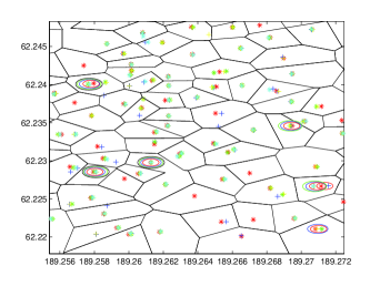
Figure 2: Examples of implementation of an iterative procedure for multi-wavelength cross-matching in the Hubble Deep Field image.

In APJ.679:301-309 , Budavari et al propose an iterative procedure based on the thresholding of the Bayes factor computed from equations 1 and 2 for the identification of counterparts in several catalogues. We have implemented this procedure and tested it with five real catalogues (one catalogue from IRAC and four catalogues from SUBARU). Figure 2 shows one example of this implementation. A threshold of $B_{0}=5$ was chosen to collect all possible candidates and the low-probability ones have been weeded out in subsequent steps. A unique astrometric precision of $\sigma\leq 0.2^{{}^{\prime\prime}}$ for all catalogues has been considered.

4 Extended Bayesian inference for the consideration of non-detection

The possibility of having non-detected sources has not been taken into account so far in the formalism described above. In APJ.679:301-309 , Budavari et al. suggest one step further by thresholding a combined Bayes factor that includes the astrometric and the photometric Bayes factors. In their proposal, the photometric Bayes factor gauges the two hypothesis that i) the photometric measurements of an $n$-tuple correspond to a single model SED (where a choice of parameterized models is available for galactic SEDs), or they come from independent and different SEDs. This allows us in general to reject a cross-matched proposal, but does not help in refining it by excluding inconsistent measurements. Here, we elaborate on that proposal in order to extract that kind of information that may allow us to construct a SED even if incomplete.

Let us take as starting point $n+1$- tuples derived from the algorithm proposed in APJ.679:301-309 which uses only astrometric information. For obvious reasons, we define the $n+1$-tuple as a set of potential counterparts to the source detected in the lowest resolution image which drives the Voronoi tessellation in celestial coordinates described in section 3. Let us define this image as $i=n+1$ in the following.

In order to include the photometric information into the inference process, we will assume that there exists a model for the galactic SED which is parametrized by the set $\{\eta_{k},k=1,2,...,K\}$. In APJ.679:301-309 , the authors parametrize each SED by a discrete spectral type $T$, the redshift $z$ and an overall scaling factor for the brightness, $\alpha$; an additional simplification which makes $\alpha=1$ can be obtained here by normalizing the SED.

It is important to note that each instrument has its own detection limit which depends, in general and amongst other factors, on the spatial flux density of a source and not on the total integrated flux; however, and for the sake of simplicity we will only consider here flux thresholds instead of fully modelling the detection process, which is always the correct approach, specially when dealing with extended sources.

The cross-matching problem described in section 3 requires the ability to identify the same source across different images with different measurement instruments. The consideration of having sources not detected under study has not been taken into account so far for the model described in APJ.679:301-309 .

Let us take as starting point $N$ tuples of n$+1$ elements derived from the algorithm proposed in APJ.679:301-309 .

For the sake of simplicity of this preliminary model, the existence of one and only one detected source in the channel which drives the voronoi tessellation in celestial coordinates described in section 3 will be assumed, therefore there will always exist a detection in this channel.

To deal with the concept of non-detection, the use of photometric information is required and for that purpose the photometric model proposed in APJ.679:301-309 will be used and extended. As indicated in arXiv:astro-ph.CO/1008.0395v1 , a wealth of models has been created with the goal of choosing and extracting useful information from SEDs. In our case we will follow the same simple model for the SED as the one indicated in APJ.679:301-309 . Let us consider the data $D^{\prime}$ as an n$+1$-tuple of the measured fluxes: $D^{\prime}=\{\vec{g_{1}},\vec{g_{2}},...,,\vec{g_{n+1}}\}$.

The Bayesian inference for this photometric model will be run on the following two mutually exclusive hypothesis:

• H₁: all the fluxes $\vec{g_{i}}$ correspond to the same source.

• K₁: not all the fluxes $\vec{g_{i}}$ correspond to the same source.

The evidences for the hypothesis H₁ and K₁ are:

$$p(D^{\prime}|H_{1})=\int p(\vec{\eta}|H_{1})\prod_{i=1}^{n+1}p_{i}(\vec{g_{i}}|\vec{\eta},H_{1})d^{r}\eta$$ (3)

where:

• $\vec{\eta}$ are the parameters for modelling the spectral energy distribution.

• $p(\vec{\eta}|H_{1})$ is the prior probability which should be carefully chosen from one of the models proposed in arXiv:astro-ph.CO/1008.0395v1 , for example, SWIRE database could be a good option for IRAC catalogues.

• $p_{i}(\vec{g_{i}}|\vec{\eta},H_{1})$ is the probability that one source with SED parameters $\vec{\eta}$ has a measured flux of $\vec{g_{i}}$.

For hypothesis K₁ we will take on board the consideration for the possibilities of having sources non-detected in one or several channels. This means that the hypothesis K₁ contains a combinatorial number of sub-hypothesis (i.e. that the source has not been detected in any possible combination of channels, and that the detections in these channels correspond to nearby sources in the celestial sphere).

In this way, one new sub-hypothesis is established per combination found; therefore there will be:

• $C_{n,1}=n$ sub-hypothesis for one non-detection.

• $C_{n,p}=\frac{n!}{p!\cdot(n-p)!}$ sub-hypothesis for p non-detections.

• $C_{n,n}=1$ sub-hypothesis for n non-detections.

The formalism proposed here for the hypotheis K₁ will include all the independent sub-hypothesis described before.

Let us be $P_{n,p}=\{L_{\{i_{1},...,i_{p}\}}\}$ the set of sub-hypothesis with $p$ non-detections and with $n-p$ detections.

The generic expression for hypothesis K₁, taking on board all the possibilities of non-detections from an n+1-tuple is as follows:

$$p(D^{\prime}|K_{1})=\prod_{i=1}^{n+1}\left\{\int p(\vec{\eta_{i}}|L)\cdot p_{i}(\vec{g_{i}}|\vec{\eta_{i}},L)d^{r}\eta_{i}\right\}$$ (4)

$$=\sum_{p=1}^{n}\sum_{L\in P_{n,p}}\prod_{i=\{i_{1},...,i_{p}\}}\left\{\int\int_{-\infty}^{\theta_{thi}}p_{i}(\vec{g_{i}}|\eta_{i},L)p(\vec{\eta_{i}}|L)d\vec{g_{i}}d^{r}\eta_{i}\right\}\cdot\prod_{j=1,j\neq i}^{j=n+1}\left\{\int p(\vec{\eta}|L)\cdot p_{j}(\vec{g_{j}}|\vec{\eta},L)d^{r}\eta\right\}$$

Where the non-detection for the source $i$ can be modelled as the area below the detection threshold, $\theta_{thi}$, of a Gaussian distribution.

The evidence for hypothesis K₁, as expressed in equation 4, includes the combinatorial number of the exclusive sub-hypothesis presented before. In this way, an unambiguous description of each specific combination of non-detection(s) among the channels of the n$+1$-tuple is feasible.

The use of the different Bayes Factors per sub-hypothesis will allow the identification of the most favourable model; alternatively other statistics as the Bayesian Model Averaging (BMA) can also provide the assessment on how probable is a model given the data conditionally on a set of models considered, L₁,…,L_p,…,L_n, being L_p the set of sub-hypothesis corresponding to $p$ non-detections. Initially we would assign the same value for each sub-hypothesis.

5 Toy example

Let us model the radiation of a black body using Planck’s law. This function depends on the frequency $\nu$.

$$I(\nu,T)=\frac{2h\nu^{5}}{c^{3}}\cdot\frac{1}{e^{\frac{h\nu}{KT}}-1}$$ (5)

Let us consider a set of measurements $g_{i}$ of the black body intensities $I(\nu,T)$, therefore for a 6-tuple we will have the following data: $D^{\prime}=\{g_{1},....g_{6}\}$; for the prior we will use a flat function as a first approximation and we will assume a Gaussian distribution for the uncertainties measurement $p_{i}(g_{i}|T)$. Note that in this case the example has been modelled in such a way that the measurement in channel $3$, $g_{3}$, will not correspond to the cross-matching.

Applying equations 3 and 4 we obtain the following Bayes factor:

$$B=\frac{p(D|H_{1})}{p(D|K_{1})}=1.92\cdot 10^{-2}$$ (6)

Therefore the model K₁ will be clearly more favourable than the model H₁. We can go a step further by applying here the extended Bayesian formalism presented, from which the Bayes Factors of all possible sub-hypothesis are obtained, resulting sub-hypothesis $L_{\{3\}}$ the most favourable one, as expected.

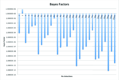
Figure 3: Bayes Factors for all sub-hypothesis included in the hypothesis $K_{1}$

6 Conclusions

The proposed extended Bayesian formalism for the probabilistic cross-matching problem drives the identification of the most favourable model among many when all the posible exclusive combinations of having non-detected sources within the n$+1$-tuple are taken into account; this stage leads to an obvious refinement phase in the construction of consistent SEDs, allowing a more precise labelling process for sources detected in multi-wavelength deep images of cosmological fields.

References

- (1) Tamas Budavari and Alexander S. Szalay: Probabilistic Cross-Identification of Astronomical Sources, The American Astronomical Society. 2008, May 20.
- (2) E. Bertin and S.Arnouts: SExtractor: Software for source extraction. Institut d’Astrophysique de Paris, France, European Southern Observatory, Chile.
- (3) M. R. Calabretta and E.W. Greisen: Representations of celestial coordinates in FITS (ESO 2002) doi: 10.1051/0004-6361:20021327
- (4) G.D’Agostini: Bayesian Inference in Processing Experimental Data. Principles and Basic Applications, Universita La Sapienza and infn, Roma, Italia, 2003
- (5) Roberto Trotta: Bayes in the sky: Bayesian inference and model selection in cosmology, Oxford University, Astrophysics Department, Denys Wilkinson Building, Keble Rd, Oxford, OX1 3RH, UK, March 28,2008.
- (6) Jakob Walcher.Brent Groves.Tamas Budavari.Daniel Dale: Fitting the integrated Spectral Energy Distributions of Galaxies, Research and Scientific Supporot Department, European Space Agency, Keplerlaan 1, 2200AG Noordwijk, The Netherlands, Sterrewacht Leiden, Leiden University, P.O. Box 9513, 2300 RA Leiden, The Netherlands, Dept. of Physics and Astronomy, The Johns Hopkins University, 3400 N. Charles Street, Baltimore, MD 21218, USA, Dept. of Physics and Astronomy, University of Wyoming, Laramie, WY 82071, USA. 2010