Revisiting the D-iteration method: from theoretical to practical computation cost
Abstract
In this paper, we revisit the D-iteration algorithm in order to better explain its connection to the Gauss-Seidel method and different performance results that were observed. In particular, we study here the practical computation cost based on the execution runtime compared to the theoretical number of iterations. We also propose an exact formula of the error for PageRank class of equations.
category:
G.1.3 Mathematics of Computing Numerical Analysiskeywords:
Numerical Linear Algebracategory:
G.2.2 Discrete Mathematics Graph Theorykeywords:
Graph algorithmskeywords:
Numerical computation; Iteration; Fixed point; Gauss-Seidel; Eigenvector.1 Introduction
2 Connection to Gauss-Seidel iteration
We recall the equation on the history vector associated to the D-iteration method:
| (1) |
where is the identity matrix, a matrix with all entries equal to zero except for the -th diagonal term: , the initial condition vector (equal to ) and the -th choice of node for the diffusion. The choice of the sequence with is the main optimization factor of the D-iteration.
The above equation (1) is in fact equivalent to:
which is exactly the Gauss-Seidel iteration equation if we apply the diagonal term elimination (division by ). This means that the history vector we obtain with the D-iteration is exactly the same results than the Gauss-Seidel’s result when applying the same sequence . In particular, it means that one can apply the Gauss-Seidel method for any infinite sequence of and the limit is not modified. However, the main difference is that with the D-iteration, we don’t use the equation (1). Instead, we use the column vector to update (, ): the advantage of introducing and working with is that (cf. pseudo-code [3]):
-
•
we know exactly in advance the amount of fluid on which the diffusion is applied (so the consequence in advance: how much remains and how much disappears): if from (and line vector application), we want to optimize the way the sequence is built, it is not obvious (and this explains why up to now only the cyclic iteration is done) and it would in fact require the information of ;
-
•
the computation cost is reduced: this will be illustrated below. The main reason is that when the diffusion is applied, each computation is useful (each diffusion adds fluid effectively to its children nodes), whereas with the line vector application on , we may have a lot of redundant computation. To understand this last idea, assume that % of are constant or almost constant. With the line vector application, there will be % of operations that will be repeated and that could be avoided if the diffusion approach is applied (cf. results comparison of Section 4.7).
3 Improving the error estimate
It has been shown in [4] that is an exact distance (for norm) to the limit when has all columns summing-up tp . In case of the PageRank equation, we may have zero-column vector in (if we don’t do the completion operation cf. [5]). Indeed if zero-column vector of (corresponding to dangling nodes) is to be completed by , any iteration scheme would do useless computations. When, we are working on the matrix without completion, the limit we obtain need to be renormalized (by a constant multiplication for diffusion approach or by constant addition for power iteration).
To take into account this effect precisely, we count the total amount of fluid that left the system when a diffusion is applied on a dangling node: we call this quantity (at step of the D-iteration). This quantity should have been put in the system by adding on each node, which means that the initial fluid should have been instead of . But then the fluid would have produced after steps that disappears by dangling nodes, etc. Applying the argument recursively, the correction that is required on the residual fluid (equal to ) is to replace the initial condition by:
And need to be renormalized (multiplication) by so that the exact distance is equal to:
Below, in the D-iteration approach, we updated by:
if is a dangling node.
4 Analysis of the computation cost
4.1 Web graph dataset
For the evaluation purpose, we used the
web graph imported from the dataset uk-2007-05@1000000
(available on [1]) which has
41,247,159 links on 1,000,000 nodes.
Below we vary from to extracting from the dataset the information on the first nodes. Few graph properties are summarized in Table 1:
-
•
L: number of non-null entries (links) of ;
-
•
D: number of dangling nodes (0 out-degree nodes);
-
•
E: number of 0 in-degree nodes: the 0 in-degree nodes are defined recursively: a node , having incoming links from nodes that are all 0 in-degree nodes, is also a 0 in-degree node; from the diffusion point of view, those nodes are those who converged exactly in finite steps;
-
•
O: number of loop nodes ();
-
•
(maximum in-degree, the in-degree of is the number of non-null entries of the -th line vector of );
-
•
(maximum out-degree, the out-degree of is the number of non-null entries of the -th column vector of ).
| N | L/N | D/N | E/N | O/N | ||
|---|---|---|---|---|---|---|
| 12.9 | 0.041 | 0.032 | 0.236 | 716 | 130 | |
| 12.5 | 0.008 | 0.145 | 0.114 | 7982 | 751 | |
| 31.4 | 0.027 | 0.016 | 0.175 | 34764 | 3782 | |
| 41.2 | 0.046 | 0 | 0.204 | 403441 | 4655 |
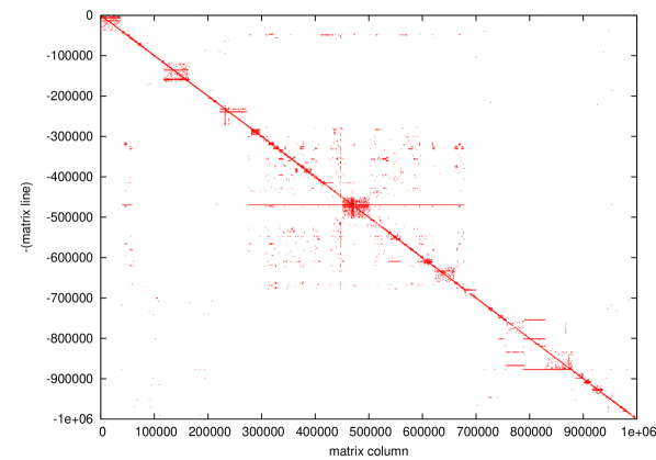
4.2 Programming environment
For the evaluation of the computation cost, we used codes () on a Linux (Ubuntu) machine:
Intel(R) Core(TM)2 CPU, U7600, 1.20GHz, cache size 2048 KB.
The runtime has been measured based on the library time.h with the function (with a precision of 10 ms). The runtime below measures the computation time from the time we start iterations (time to build the iterators are excluded).
4.3 First comparison tests
The first algorithms that we evaluated in this section are:
-
•
PI: Power iteration (equivalent to Jacobi iteration);
-
•
GS: Gauss-Seidel iteration (cyclic sequence);
-
•
GS’: Gauss-Seidel iteration (cyclic sequence): keeping diagonal terms;
-
•
DI-CYC: D-iteration with cyclic sequence (a node is selected, if );
-
•
DI-MAX: D-iteration with by threshold (by threshold means that we apply the diffusion to all nodes above the threshold value; when there is no such node, we decrease multiplicatively the threshold, by default by 1.2, which we call the decrement factor);
-
•
DI-OP: D-iteration with by threshold, diffusions are applied first on the 0 in-degree nodes (recursively, such that we need to apply the diffusion exactly once to each of those nodes).
Because, we are currently limited by the memory size on a single PC, we introduced an arbitrary function each time a non zero entry of need to be used by introducing a finite iteration of
void ArbitraryFunction(int m){
double x = 1.0;
for (int i=0; i < m; i++){
x := a * x + b;
}
}
( is the number of times we iterates): this would correspond exactly to the reality if the operation is to be replaced by an operator whose computation cost is exactly the finite iteration we introduced arbitrarily.
As one can observe in the results of Tables 2 and 3, the main improvements are brought by:
-
•
coordinate level update with the iteration GS and DI-CYC (against vector level update of PI);
-
•
a better choice of the nodes for the diffusion process: we see a significant jump with the very basic solution DI-MAX;
-
•
then with DI-OP (we observed similar improvements with all variants of the idea of the argmax of weighted fluid).
The impact of the diagonal term elimination and the impact of the redundant computation of line-vector operations in GS is limited here.
We see also that the computation cost estimate with the number of iterations is a very good approximation when the matrix product operations (the multiplications) are the dominant component of the computation run time cost (when is introduced).
When we set (real runtime), we see that the real speed-up gain may be in fact much more important than those estimates (for large ). Also, we can notice a surprising efficiency of DI-CYC: if the main speed-up gain is from DI-MAX for the number of iterations, the maim improvement is brought by DI-CYC for the runtime.
| PI | GS’ | DI-CYC | DI-MAX | DI-OP | |
|---|---|---|---|---|---|
| nb iter | 28 | 22 | 20.8 | 14.4 | 12.8 |
| speed-up | 1.0 | 1.3 | 1.4 | 1.9 | 2.2 |
| time (s) | 303 | 238 | 225 | 157 | 138 |
| speed-up | 1.0 | 1.3 | 1.4 | 1.9 | 2.2 |
| time (s) | 0.02 | 0.02 | 0.02 | 0.02 | 0.02 |
| speed-up | 1.0 | 1.0 | 1.0 | 1.0 | 1.0 |
| nb iter | 43 | 38 | 34.9 | 17.2 | 13.8 |
| speed-up | 1.0 | 1.1 | 1.2 | 2.5 | 3.1 |
| time (s) | 453 | 401 | 367 | 181 | 146 |
| speed-up | 1.0 | 1.1 | 1.2 | 2.5 | 3.1 |
| time (s) | 0.29 | 0.28 | 0.13 | 0.23 | 0.11 |
| speed-up | 1.0 | 1.0 | 2.2 | 1.3 | 2.6 |
| nb iter | 52 | 43 | 42.9 | 21.1 | 16.2 |
| speed-up | 1.0 | 1.2 | 1.2 | 2.5 | 3.2 |
| time (s) | 1386 | 1146 | 1131 | 560 | 431 |
| speed-up | 1.0 | 1.2 | 1.2 | 2.5 | 3.2 |
| time (s) | 9.0 | 8.0 | 2.7 | 3.6 | 2.1 |
| speed-up | 1.0 | 1.1 | 3.3 | 2.5 | 4.3 |
| nb iter | 66 | 57 | 57 | 18.3 | 15.7 |
| speed-up | 1.0 | 1.2 | 1.2 | 3.6 | 4.2 |
| time (s) | 2639 | 2275 | 2051 | 693 | 586 |
| speed-up | 1.0 | 1.2 | 1.3 | 3.8 | 4.5 |
| time (s) | 223 | 198 | 45 | 49 | 27 |
| speed-up | 1.0 | 1.1 | 5.0 | 4.6 | 8.3 |
| PI | GS | DI-CYC | DI-MAX | DI-OP | |
|---|---|---|---|---|---|
| nb iter | 28 | 18.7 | 17.5 | 13.3 | 11.3 |
| speed-up | 1.0 | 1.5 | 1.6 | 2.1 | 2.5 |
| time (s) | 303 | 202 | 190 | 144 | 123 |
| speed-up | 1.0 | 1.5 | 1.6 | 2.1 | 2.5 |
| time (s) | 0.02 | 0.02 | 0.02 | 0.02 | 0.02 |
| speed-up | 1.0 | 1.0 | 1.0 | 1.0 | 1.0 |
| nb iter | 43 | 30.7 | 26.4 | 16.0 | 12.2 |
| speed-up | 1.0 | 1.4 | 1.6 | 2.7 | 3.5 |
| time (s) | 453 | 324 | 277 | 170 | 129 |
| speed-up | 1.0 | 1.4 | 1.6 | 2.7 | 3.5 |
| time (s) | 0.29 | 0.23 | 0.10 | 0.17 | 0.09 |
| speed-up | 1.0 | 1.3 | 2.9 | 1.7 | 3.2 |
| nb iter | 52 | 36.8 | 34.7 | 20.1 | 15.5 |
| speed-up | 1.0 | 1.4 | 1.5 | 2.6 | 3.4 |
| time (s) | 1386 | 981 | 915 | 531 | 410 |
| speed-up | 1.0 | 1.4 | 1.5 | 2.6 | 3.4 |
| time (s) | 9.0 | 6.9 | 2.1 | 3.6 | 1.9 |
| speed-up | 1.0 | 1.3 | 4.3 | 2.5 | 4.7 |
| nb iter | 66 | 41.8 | 39.8 | 17.8 | 15.3 |
| speed-up | 1.0 | 1.6 | 1.7 | 3.7 | 4.3 |
| time (s) | 2639 | 1670 | 1431 | 670 | 567 |
| speed-up | 1.0 | 1.6 | 1.8 | 3.9 | 4.7 |
| time (s) | 223 | 147 | 31 | 44 | 36 |
| speed-up | 1.0 | 1.5 | 7.2 | 5.1 | 6.0 |
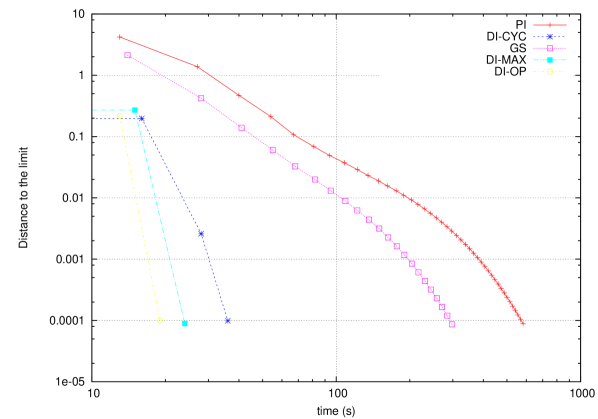
Figure 2 and 3 shows the evolution of the distance to the limit w.r.t. the computation costs: as we said, we can observe that the number of iterations is a very good estimate of the real cost when the multiplication operations with the entries of the matrix is the dominant component of the computation.
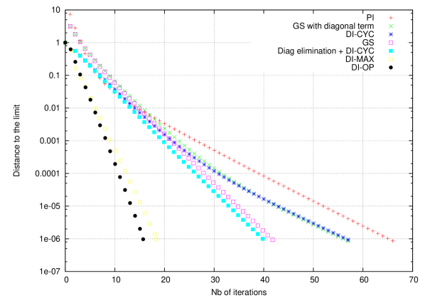
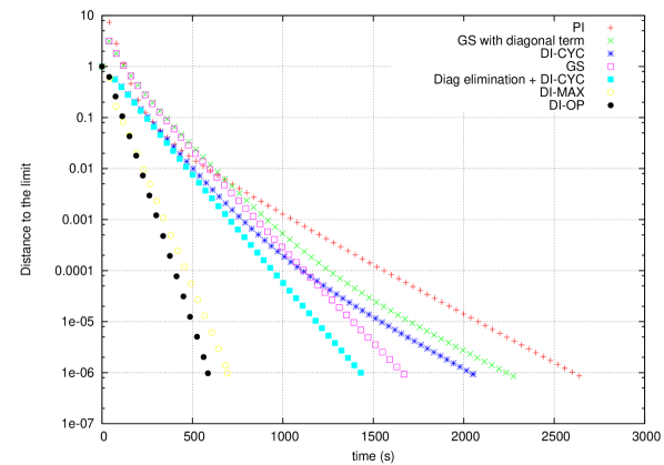
The visible difference in the number of iterations and runtime for DI-CYC we noticed above can be explained by the fact that for the practical numerical computation point of view, it is not necessarily good to look for the optimal sequence: instead of spending time to select the best nodes for the diffusion, it suggests that it would be better to choose quickly suboptimal nodes for the diffusion: the simplest is DI-CYC, but we’ll see that we can do better.
4.4 Second comparison tests
Based on the first observation, we next re-evaluated the computation cost, decreasing the cost of the node selection: or by increasing the threshold decrement factor (DI-OP2, DI-MAX2) or by taking all nodes above a certain average (and not choosing the threshold from the maximum) with DI-OP3, with the idea of wasting less time to find the optimal nodes for diffusion. Below, the different algorithms for the second tests:
-
•
DI-OP: D-iteration with by threshold (decrement factor 1.2), diffusions are applied first on the O in-degree nodes (recursively, such that they need to send exactly once);
-
•
DI-OP2: as DI-OP, decrement factor 10.0;
-
•
DI-OP3: D-iteration with node selection if ; the value is the remaining fluid value computed by cycle ;
-
•
DI-MAX2: as DI-MAX, with node selection if ;
When simplifying the node selection method, we obtain results presented in Table 4. We see that DI-OP3 is a good compromise between the number of iterations reduction and runtime reduction. Note that the results of DI-MAX2 clearly shows a poor performance of the runtime w.r.t. what is expected from the number of iterations: the reason is that the number of nodes having fluid above the value is not important and we end up spending a lot of time testing the node selection condition. And this explains also why DI-OP3 works better (less useless test operations) for the runtime, whereas for the number of iterations, DI-MAX2 and DI-OP3 are much closer.
| DI-OP | DI-OP2 | DI-OP3 | DI-MAX2 | |
| nb iter | 12.2 | 17.1 | 12.9 | 13.0 |
| time | 0.09 | 0.09 | 0.09 | 0.11 |
| nb iter | 15.5 | 20.2 | 15.7 | 18.3 |
| time | 1.9 | 1.6 | 1.5 | 2.9 |
| nb iter | 15.3 | 20.4 | 15.8 | 15.8 |
| time | 36 | 20 | 18 | 39 |
Table 5 gives the runtime comparison of different approach when we eliminate all operations indirectly linked to the iterations, such as normalization, convergence test (only kept for DI-OP3) and printing results (time2). We see that its impact (time2 compared to time1) can be neglected for PI, GS and DI-CYC, much less for DI-MAX2 and DI-OP3. We see that for , we can improve PI by factor 15 and GS by factor 10. This gain factor is much more than the ratio on the number of iterations. In order to explain this difference, we also introduced time3, which is the runtime obtained when at the compilation level of the source code () the optimization option () was not used. We see that the results are closer to the predicted values from the number of iterations. However, we still observe a difference of about a factor 2 on DI variants.
| PI | GS | DI-CYC | DI-MAX2 | DI-OP3 | |
| nb iter | 43 | 30.7 | 26.4 | 13.0 | 12.9 |
| time1 (s) | 0.29 | 0.23 | 0.10 | 0.11 | 0.09 |
| time2 (s) | 0.26 | 0.21 | 0.07 | 0.09 | 0.05 |
| time3 (s) | 0.83 | 0.65 | 0.40 | 0.45 | 0.24 |
| nb iter | 52 | 36.8 | 34.7 | 18.3 | 15.7 |
| time1 (s) | 9.0 | 6.9 | 2.2 | 2.9 | 1.5 |
| time2 (s) | 8.8 | 6.8 | 1.9 | 2.5 | 1.1 |
| time3 (s) | 25.9 | 18.1 | 11.1 | 12.4 | 5.6 |
| nb iter | 66 | 41.8 | 39.8 | 15.8 | 15.8 |
| speed-up | 1 | 1.6 | 1.7 | 4.2 | 4.2 |
| time1 (s) | 223 | 147 | 31 | 39 | 18 |
| time2 (s) | 221 | 147 | 29 | 31 | 14.4 |
| speed-up | 1 | 1.5 | 7.6 | 7.1 | 15.3 |
| time3 (s) | 496 | 323 | 164 | 169 | 70 |
| speed-up | 1 | 1.5 | 3.0 | 2.9 | 7.1 |
4.5 Further analysing the speed-up factors
We first shows in Figures 4 and 5 the evolution of the speed-up factor with for different approaches. We observe a quite promising trend of speed-up factor for the runtime: Figure 5 shows that the gain factor due to the sequence choice is significantly increasing with the size .
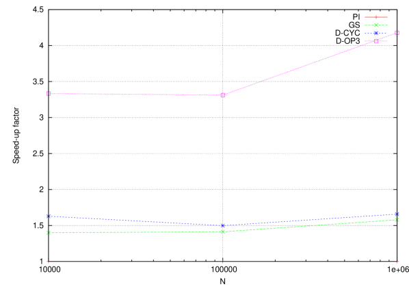
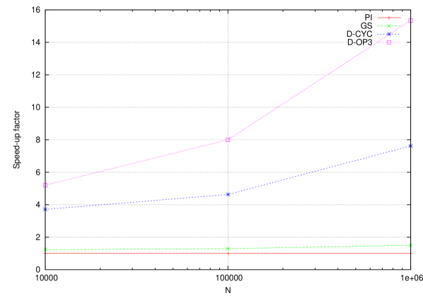
For the considered matrix associated to the web graph, we can approximately decompose the speed-up gain factor for as follows (for runtime):
-
•
Entry level update (GS): factor 1.5;
-
•
Use of (all) column vectors instead of (all) line vectors: factor 3 (compilation/processor optimization, cache memory management); this factor is highly dependent on the structure of the graph and the compilation optimization (with Java code, we observed very different performance); this factor may be less than one (for instance if -transposition of - is to be considered);
-
•
Impact of sequence choice: factor 4:
-
–
take columns with positive fluid (DI-CYC): factor 2;
-
–
better selected choice of columns (DI-OP3): factor 2.
-
–
As we observed in the previous section, there is a significant gap between the computation cost in runtime or in number of iterations. We suspect that the main reason comes from a factor relative to the compilation level (as we saw, such as the optimization option), or the way the processor manages the cache memory access. To validate our assumption, we did the following tests: we evaluated the impact of the use of the column or line vectors of in terms of the runtime. On the case , we run the codes for column and line iterators:
Code for line iterator:
double result = 0.0;
double count = 0;
while ( count < 100 ){
count++;
for (int i = 0; i < N; i++){
for (list<int>::iterator j = line[i].begin();
j != line[i].end(); j++){
result += *j;
}
}
}
where line[i] is the iterator on the -th line of ().
Code for column iterator:
double result = 0.0;
double count = 0;
while ( count < 100 ){
count++;
for (int i = 0; i < N; i++){
for (list<int>::iterator j = column[i].begin();
j != column[i].end(); j++){
result += *j;
}
}
}
where column[i] is the iterator on the -th column of ().
By iterating the above schemes, we obtained a runtime of 21 (line) and 6 (column) seconds (difference of factor 3.3). When the compilation option is not used, we observed quite close results. The reason of this difference may be in the property of the graph: Figure 6 shows the number of incoming and outgoing links per node position. We clearly see that the variance of the number of outgoing links is much more smaller than the variance of the number of incoming links. We can expect such a property may be quite general when the graph is built from human contributions: the outgoing links of a node are likely to be produced by one person or a small group of persons. Whereas when a web site or a content is very popular, it may receive a huge number of incoming links (following a popularity law such as Zipf’s law).
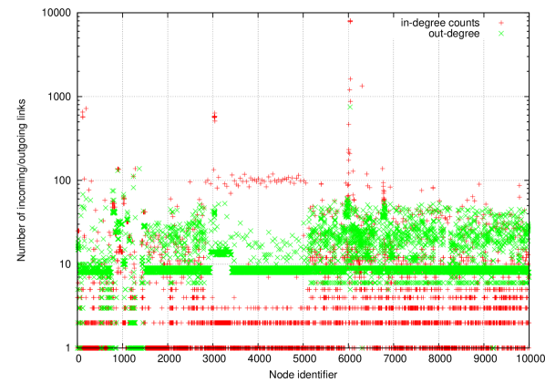
This means that for the operations with the line vector (collection), we end up with lists of very variable sizes. The operations with the column vector (diffusion) require lists of more regular sizes with less variance.
For a better clarification of the runtime speed-up results, we consider now the different algorithms for the matrix (transposition of ). If the above explanation is consistent, we should have line-iterator operations much faster than column-iterator operations. The results are shown in Table 6: they are roughly as expected. If the gain factor from the line or column iteration is about 3.3, taking the we should have an impact of about and this is what we observe on the ratio (time1 for DI-OP3). This is of course a very approximative explanation since the behaviours of the compiler and of the processor are very complex.
| PI | GS | DI-CYC | DI-OP3 | |
|---|---|---|---|---|
| nb iter | 66/78 | 42/46 | 40/43 | 16/42 |
| speed-up | 1/1 | 1.6/1.5 | 1.7/1.6 | 4.1/1.6 |
| time1 (s) | 223/99 | 147/59 | 31/165 | 18/176 |
| speed-up | 1/1 | 1.5/1.7 | 7.2/0.6 | 16.7/0.6 |
| time3 (s) | 496/388 | 323/244 | 164/291 | 70/284 |
| speed-up | 1/1 | 1.5/1.6 | 3.0/1.3 | 7.1/1.4 |
4.6 A sub-optimal scheme
Based on the above results, we understood that in the real computation cost of the iteration scheme, the optimization of the iterator plays an important role. In particular, when we have a column of with a too large number of non-zero entries, its diffusion should be carefully controlled (limit as much as possible). This helped us to define the following scheme:
-
•
DI-SOP (sub-optimal compromise solution): D-iteration with node selection, if , where is the out-degree of and is computed per cycle .
| PI | GS | DI-CYC | DI-SOP | |
|---|---|---|---|---|
| nb iter | 52/51 | 37/38 | 35/35 | 14/17 |
| speed-up | 1/1 | 1.4/1.3 | 1.5/0.5 | 3.7/3.0 |
| time1 (s) | 9.0/5.0 | 6.9/3.8 | 2.2/7.2 | 1.0/3.6 |
| speed-up | 1/1 | 1.3/1.3 | 4.1/0.7 | 9.0/1.4 |
| time3 (s) | 26/20 | 18/16 | 11/15 | 5/8 |
| speed-up | 1/1 | 1.4/1.2 | 2.3/1.3 | 5.6/2.5 |
| nb iter | 66/78 | 42/46 | 40/43 | 14/17 |
| speed-up | 1/1 | 1.6/1.7 | 1.7/1.8 | 4.7/4.6 |
| time1 (s) | 223/99 | 147/59 | 31/165 | 13.2/50 |
| speed-up | 1/1 | 1.5/1.7 | 7.2/0.6 | 16.9/2.0 |
| time3 (s) | 496/388 | 323/244 | 164/291 | 59.4/107 |
| speed-up | 1/1 | 1.5/1.6 | 3.0/1.3 | 8.4/3.6 |
Table 7 shows that DI-SOP performs pretty robustly even in worst conditions (). The intuition of DI-SOP is very clear: we choose all nodes such that the unitary diffusion cost is above the average diffusion cost . Indeed, can be decomposed as (average fluid per node) divided by (average out-degree).
| PI | GS | DI-CYC | DI-SOP | |
|---|---|---|---|---|
| nb iter | 54 | 31.4 | 29.1 | 18.2 |
| speed-up | 1.0 | 1.7 | 1.9 | 3.0 |
| time (s) | 0.63 | 0.38 | 0.34 | 0.20 |
| speed-up | 1.0 | 1.7 | 1.9 | 3.1 |
| nb iter | 67 | 44.6 | 39.0 | 17.8 |
| speed-up | 1.0 | 1.5 | 1.7 | 3.8 |
| time (s) | 1.44 | 0.99 | 0.62 | 0.30 |
| speed-up | 1.0 | 1.5 | 2.3 | 4.8 |
| nb iter | 77 | 50.7 | 48.6 | 20.0 |
| speed-up | 1.0 | 1.5 | 1.6 | 3.9 |
| time (s) | 14.6 | 11.1 | 4.3 | 2.5 |
| speed-up | 1.0 | 1.3 | 3.4 | 5.8 |
| nb iter | 92 | 55.7 | 53.7 | 19.5 |
| speed-up | 1.0 | 1.7 | 1.7 | 4.8 |
| time (s) | 309 | 194 | 41.5 | 20.0 |
| speed-up | 1.0 | 1.6 | 7.4 | 15 |
Table 8 summarizes the results of the comparison for different , introducing only for differentiation purpose. Table 9 shows the results obtained when we set a large value of damping factor (this makes the global convergence speed slower): the difference of performance is better illustrated: it seems that there is more gain when more iterations are required (we could guess it from Figure 3: only DI-variants are linear). With , we gained here a factor 36 in runtime.
| PI | GS | DI-CYC | DI-SOP | |
|---|---|---|---|---|
| nb iter | 399 | 303 | 268 | 111 |
| speed-up | 1.0 | 1.3 | 1.5 | 3.6 |
| time (s) | 0.17 | 0.15 | 0.09 | 0.03 |
| speed-up | 1.0 | 1.1 | 1.9 | 5.7 |
| nb iter | 544 | 480 | 404 | 71.3 |
| speed-up | 1.0 | 1.1 | 1.3 | 7.6 |
| time (s) | 3.46 | 3.45 | 1.36 | 0.29 |
| speed-up | 1.0 | 1.0 | 2.5 | 12 |
| nb iter | 790 | 579 | 543 | 117 |
| speed-up | 1.0 | 1.4 | 1.5 | 6.8 |
| time (s) | 137 | 107 | 34 | 9.2 |
| speed-up | 1.0 | 1.3 | 4.0 | 15 |
| nb iter | 1028 | 648 | 614 | 98 |
| speed-up | 1.0 | 1.6 | 1.7 | 10 |
| time (s) | 3455 | 2257 | 480 | 95 |
| speed-up | 1.0 | 1.5 | 7.2 | 36 |
We globally observe that when a sufficiently large is used, the relative computation time to PI is close to the prediction (number of iterations ratio) at least for GS and DI-CYC. For , it seems that the computation time gain relative to PI for DI-variants may be higher then the prediction when is effectively large (for and with [1]), possibly due to the cache memory access time optimization by the processor (likely to have fewer elements in the cache with D-variants): the impact of the compilation or the processor level optimization is clearly very important, but this is another complex research issue which is out of scope of this paper. We hope to address this problem in a future work.
4.7 Revisiting another dataset
Below, we used the web graph gr0.California
(available on http://www.cs.cornell.edu/Courses/cs685/ 2002fa/).
The main motivation was here to try to understand the unexpected (too much) gain
observed in [4] for this graph.
| L/N | D/N | E/N | O/N | ||
|---|---|---|---|---|---|
| 1.67 | 0.48 | 0.91 | 0 | 199 | 164 |
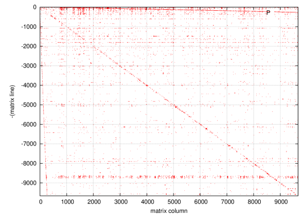
As Table 10 shows, this graph is very specific in that more than 90% of nodes are 0 in-degree nodes. This is quite interesting, because it illustrates clearly here the difference between collection (line vector use) or diffusion (column vector use) approaches: because the 0 in-degree nodes converges in finite iterations, GS is recomputing 90% of redundant operations, whereas with the diffusion approach, the 0 in-degree nodes are very easily identified as nodes having 0 fluid and DI-CYC will only apply diffusion on 10% of nodes, explaining the gain factor of almost 10 between PI/GS and DI-CYC (Table 11).
| PI | GS | DI-CYC | DI-OP3 | DI-SOP | |
|---|---|---|---|---|---|
| nb iter | 43 | 22 | 3.1 | 1.6 | 1.6 |
| speed-up | 1 | 2 | 14 | 27 | 27 |
| time1 | 582 | 298 | 42 | 9.2 | 12.2 |
| speed-up | 1 | 2.0 | 14 | 63 | 48 |
| time2 | 0.06 | 0.04 | 0.03 | 0.02 | 0.01 |
| speed-up | 1 | 1.5 | 2.0 | 3.0 | 6.0 |
| time3 | 0.16 | 0.13 | 0.04 | 0.02 | 0.03 |
| speed-up | 1 | 1.2 | 4.0 | 8.0 | 5.3 |
Table 12 presents the results of the computation cost associated to the matrix for comparison.
| PI | GS | DI-CYC | DI-OP3 | DI-SOP | |
|---|---|---|---|---|---|
| nb iter | 28 | 16 | 5.6 | 2.0 | 1.8 |
| speed-up | 1 | 1.8 | 5.0 | 14 | 16 |
| time1 | 379 | 217 | 75.2 | 17.7 | 9.3 |
| speed-up | 1 | 1.7 | 5.0 | 21 | 40 |
| time2 | 0.04 | 0.04 | 0.02 | 0.02 | 0.01 |
| speed-up | 1 | 1.0 | 2.0 | 2.0 | 4.0 |
| time3 | 0.11 | 0.10 | 0.05 | 0.04 | 0.03 |
| speed-up | 1 | 1.1 | 2.2 | 2.8 | 3.7 |
5 Conclusion
In this paper we revisited the D-iteration method with a practical consideration of the computation cost: step-by-step, we tried to understand and analyse the different components in the runtime cost. This led us to a more practical solution DI-SOP which seems to be a very good heuristic candidate for the choice of the sequence for the diffusion.
References
- [1] http://law.dsi.unimi.it/datasets.php.
- [2] G. H. Golub and C. F. V. Loan. Matrix Computations. The Johns Hopkins University Press, 3rd edition, 1996.
- [3] D. Hong. D-iteration method or how to improve gauss-seidel method. arXiv, http://arxiv.org/abs/1202.1163, February 2012.
- [4] D. Hong. Optimized on-line computation of pagerank algorithm. submitted, http://arxiv.org/abs/1202.6158, 2012.
- [5] A. N. Langville and C. D. Meyer. Deeper inside pagerank. Internet Mathematics, 1(3), 2004.
- [6] Y. Saad. Iterative Methods for Sparse Linear Systems. Society for Industrial and Applied Mathematics, Philadelphia, PA, USA, 2nd edition, 2003.