Theory of frequency-filtered and time-resolved
$N$-photon correlations

Abstract

A theory of correlations between $N$ photons of given frequencies and detected at given time delays is presented. These correlation functions are usually too cumbersome to be computed explicitly. We show that they are obtained exactly through intensity correlations between two-level sensors in the limit of their vanishing coupling to the system. This allows the computation of correlation functions hitherto unreachable. The uncertainties in time and frequency of the detection, which are necessary variables to describe the system, are intrinsic to the theory. We illustrate the power of our formalism with the example of the Jaynes–Cummings model, by showing how higher order photon correlations can bring new insights into the dynamics of open quantum systems.

Photons emerged as a theoretical concept to explain fundamental properties of the electromagnetic field, such as the relationship between the energy of light and its frequency, thermal equilibrium of light and matter or the photo-electric effect. With the advances in the generation, emission, transmission and detection of photons, quantum systems are increasingly addressed at the single photon level and there is a pressing need for generalizations as well as refinements of the theory of photo-detection Vogel and Welsch (2006). For instance, photon correlations combining both their frequency and time information are now routinely measured in the laboratory. These experiments have proven extremely powerful in characterising quantum systems such as a resonantly driven emitter Aspect et al. (1980); Schrama et al. (1991); Ulhaq et al. (2012), the strong coupling of light and matter Press et al. (2007); Hennessy et al. (2007); Kaniber et al. (2008), to perform quantum state tomography Akopian et al. (2006), to monitor heralded single photon sources Moreau et al. (2001) or to access spectral diffusion of single emitters Sallen et al. (2010).

At this level of fine control of the attributes of the quantum particles, one needs a theoretical description significantly more involved than general mathematical statements, such as the Wiener–Khinchin theorem which assumes abstract and unphysical properties of the light field. Eberly and Wódkiewicz, for instance, have shown how the physics of the detector needs to be included if a more realistic description of the light field is required Eberly and Wódkiewicz (1977). In general, the more detailed is the characterization of a quantum system, the more necessary it becomes to describe its measurement. A bridge between the quantum system and the observer can be made with the so-called input-output formalism: the photons inside the system, say with operator $a$ (we consider a single mode for simplicity), are weakly coupled to an outside continuum of modes, with operators $A_{\omega}$ (corresponding to their frequency $\omega$). In the Heisenberg picture, the output field allows to compute the time-dependent power spectrum of emission as the density of output photons with frequency $\omega_{1}$ at time $T_{1}$, i.e., $S^{(1)}(\omega_{1},T_{1})=\langle A^{\dagger}_{\omega_{1}}(T_{1})A_{\omega_{1}}(T_{1})\rangle$. This quantity is physical only if the uncertainties of detection in both time and frequency are jointly taken into account Eberly and Wódkiewicz (1977). Mathematically, this amounts to adding two exponential decays in the Fourier transform of the time-autocorrelation $S_{\Gamma_{1}}^{(1)}(\omega_{1},T_{1})=\frac{\Gamma_{1}}{2\pi}\iint_{-\infty}^{T_{1}}dt_{1}^{\prime}dt_{4}^{\prime}e^{-\frac{\Gamma_{1}}{2}(T_{1}-t_{1}^{\prime})}e^{-\frac{\Gamma_{1}}{2}(T_{1}-t_{4}^{\prime})}e^{i\omega_{1}(t_{4}^{\prime}-t_{1}^{\prime})}\langle{a^{\dagger}}(t_{1}^{\prime})a(t_{4}^{\prime})\rangle$ where $\Gamma_{1}$ is interpreted as the linewidth of the detector. This so-called physical spectrum reduces to the Wiener–Khinchin theorem in the steady state and in the limit $\Gamma_{1}\rightarrow 0$.

Extending this result for the detection of two photons was initially motivated by the Aspect et al. experiment Aspect et al. (1980) of resonance fluorescence in the Mollow triplet regime Mollow (1969), where the peaks of the triplet were found to exhibit strong intensity correlations. These were described theoretically at first by dedicated methods for the problem at hand, from Cohen–Tannoudji et al. (dressed atom picture) Cohen-Tannoudji and Reynaud (1979); Reynaud (1983) and Dalibard et al. (diagrammatic expansion)Dalibard and Reynaud (1983). The extension of photo-detection in the spirit of Eberly and Wódkiewicz by considering two detectors with respective linewidths $\Gamma_{1}$ and $\Gamma_{2}$ was impulsed by Knöll et al. Knöll et al. (1984) and Arnoldus and Nienhuis Arnoldus and Nienhuis (1984). The expressions were of general validity, even though, due to their complexity, the authors still focused on the particular case of resonance fluorescence for illustration. The mathematical foundations, shaky in their initial development, were firmly established in the course of the following years Knöll and Weber (1986); Knöll et al. (1986); Cresser (1987). The multiplicity of photons requires a careful time ($\mathcal{T}_{\pm}$) and normal ($:$) ordering of the operators Cresser (1987); Knöll et al. (1986), and it was realized that it is the time ordering of $\langle{:}A^{\dagger}_{\omega_{1}}(T_{1})A_{\omega_{1}}(T_{1})A^{\dagger}_{\omega_{2}}(T_{2})A_{\omega_{2}}(T_{2}){:}\rangle$ which provides the physical two-photon spectrum $S_{\Gamma_{1}\Gamma_{2}}^{(2)}(\omega_{1},T_{1};\omega_{2},T_{2})=\frac{\Gamma_{1}\Gamma_{2}}{(2\pi)^{2}}\iint_{-\infty}^{T_{1}}dt_{1}^{\prime}dt_{4}^{\prime}e^{-\frac{\Gamma_{1}}{2}(T_{1}-t_{1}^{\prime})}e^{-\frac{\Gamma_{1}}{2}(T_{1}-t_{4}^{\prime})}\iint_{-\infty}^{T_{2}}dt_{2}^{\prime}dt_{3}^{\prime}e^{-\frac{\Gamma_{2}}{2}(T_{2}-t_{2}^{\prime})}e^{-\frac{\Gamma_{2}}{2}(T_{2}-t_{3}^{\prime})}e^{i\omega_{1}(t_{4}^{\prime}-t_{1}^{\prime})}e^{i\omega_{2}(t_{3}^{\prime}-t_{2}^{\prime})}\times\langle\mathcal{T}_{-}[{a^{\dagger}}(t_{1}^{\prime}){a^{\dagger}}(t_{2}^{\prime})]\mathcal{T}_{+}[a(t_{3}^{\prime})a(t_{4}^{\prime})]\rangle$. Here, we have defined $\mathcal{T}_{+}$ (resp. $\mathcal{T}_{-}$) to order the operators in a product with the latest time to the far left (resp. far right) Vogel and Welsch (2006). Normalising this expression yields the sought time- and frequency- resolved two-photon correlation function $g_{\Gamma_{1}\Gamma_{2}}^{(2)}(\omega_{1},T_{1};\omega_{2},T_{2})=S_{\Gamma_{1}\Gamma_{2}}^{(2)}(\omega_{1},T_{1};\omega_{2},T_{2})\big{/}\big{[}S_{\Gamma_{1}}^{(1)}(\omega_{1},T_{1})S_{\Gamma_{2}}^{(1)}(\omega_{2},T_{2})\big{]}$. It is positive and finite, and reflects that frequency and time of emission cannot be both measured with arbitrary precision, in accordance with Heisenberg’s uncertainty principle. The limiting behaviours of $g_{\Gamma_{1}\Gamma_{2}}^{(2)}$ defined in this way are those expected on physical grounds: photons are uncorrelated at infinite delays, $\lim_{|T_{2}-T_{1}|\rightarrow\infty}g_{\Gamma_{1}\Gamma_{2}}^{(2)}(\omega_{1},T_{1};\omega_{2},T_{2})=1$ Glauber (1963), and color-blind detectors recover the standard two-time correlators, $\lim_{\Gamma_{1},\Gamma_{2}\rightarrow\infty}g_{\Gamma_{1}\Gamma_{2}}^{(2)}(\omega_{1},T_{1};\omega_{2},T_{2})=g^{(2)}(T_{1};T_{2})$. Further generalisation to $N$-photon correlations follows in this way, adding pairs of operators with their corresponding integrals Knöll and Weber (1986); Knöll et al. (1990).

The actual computation of such $g^{(N)}_{\Gamma_{1}\dots\Gamma_{N}}$, however, have proved so far intractable for $N>2$, even for simple single-mode systems, such as resonance fluorescence or the single mode laser Centeno Neelen et al. (1993). The case $N=2$ is already demanding and thus some approximations were made to simplify the algebra Nienhuis (1993); Joosten and Nienhuis (2000). More recently, the resonance fluorescence problem was revisited without approximations but still for two photons and at zero time delay only Bel and Brown (2009). The main reason for such limitations is that all the possible time orderings of the $2N$-time correlator $\langle\mathcal{T}_{-}[{a^{\dagger}}(t_{1}^{\prime})\dots a^{\dagger}(t_{N}^{\prime})]\mathcal{T}_{+}[a(t_{N+1}^{\prime})\dots a(t_{2N}^{\prime})]\rangle$ result in $(2N-1)!!2^{N-1}$ independent terms. Furthermore, each of these correlators requires the application of the quantum regression theorem $2N-1$ times. This growth of the complexity makes a direct computation hopeless for a quantity which is otherwise straightforward to measure experimentally, merely by detecting photon clicks as function of time and energy, a technology provided for instance by a streak camera Wiersig et al. (2009).

In this letter, we present a theory of $N$-photon correlations, that $i)$ allows for arbitrary time delays and frequencies, $ii)$ is applicable to any open quantum system and $iii)$ is both simple to implement and powerful. It consists in the introduction of $N$ sensors to the dynamics of the open quantum system (noted $Q$ in Fig. 1(a)). Each sensor of the set $i=1,\dots,N$ is a two-level system with annihilation operator $\varsigma_{i}$ and transition frequency $\omega_{i}$, that is matched to the frequency to be probed in the system. Its lifetime $1/\Gamma_{i}$ corresponds to the inverse detector linewidth. The coupling $\varepsilon_{i}$ to each sensor is small enough so that the dynamics of the system is unaltered by their presence, with $\langle n_{i}\rangle=\langle{\varsigma_{i}^{\dagger}}\varsigma_{i}\rangle\ll 1$. More precisely, calling $\gamma_{Q}$ any transition rate within $Q$ (either with internal or external degrees of freedom) linked to the field of interest $a$, the tunnelling rates $\varepsilon_{i}$ must be such that losses into the sensors and their back action are negligible, leading to $\varepsilon_{i}\ll\sqrt{\Gamma_{i}\gamma_{Q}/2}$. Under this condition, we solve the full quantum dynamics of the system supplemented with the $N$ sensors. The latter play the role of the output fields $A_{\omega_{i}}(t)$, but instead of formally solving the Heisenberg equations and expressing their correlations in terms of the system operators (as in the standard method exposed above), we compute directly intensity–intensity correlations between sensors, which is a considerably simpler task. The main result of this letter, which is demonstrated in the supplemental material, is:

$$g_{\Gamma_{1}\dots\Gamma_{N}}^{(N)}(\omega_{1},T_{1};\dots;\omega_{N},T_{N})=\lim_{\varepsilon_{1},\dots,\varepsilon_{N}\rightarrow 0}\frac{\langle n_{1}(T_{1})\dots n_{N}(T_{N})\rangle}{\langle n_{1}(T_{1})\rangle\dots\langle n_{N}(T_{N})\rangle}$$ (1)

where the left hand side is the time- and frequency-resolved $N$-photon correlation function as defined previously . The supplemental material establishes that, for open quantum systems described by Lindblad type master equations, $\langle n_{1}(T_{1})\dots n_{N}(T_{N})\rangle=\frac{\varepsilon_{1}^{2}\dots\varepsilon_{N}^{2}}{\Gamma_{1}\dots\Gamma_{N}}(2\pi)^{N}S^{(N)}_{\Gamma_{1}\dots\Gamma_{N}}(\omega_{1},T_{1};\dots;\omega_{N},T_{N})$ to leading order in the $\varepsilon_{i}$, which proves Eq. (1). The equality is of general validity with no approximations or assumptions on the system. With this result, the complexity of computing $g_{\Gamma_{1}\dots\Gamma_{N}}^{(N)}(\omega_{1},T_{1};\dots;\omega_{N},T_{N})$ is greatly reduced as no integral needs to be computed and the quantum regression theorem needs to be applied $N-1$ times only . For the important case of zero delay, $g_{\Gamma_{1}\dots\Gamma_{N}}^{(N)}(\omega_{1};\dots;\omega_{N})$ reduces to a single-time averaged quantity. $N$ degenerate sensors with frequency $\omega$ and linewidth $\Gamma$ also provide the $N$th-order correlations of a single harmonic oscillator with frequency $\omega$ and linewidth $\Gamma$, corresponding to the case of correlations measured after the application of a single filter. This method is also useful to derive analytical results (as shown in the supplemental material).

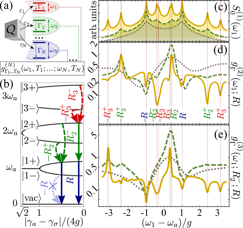
Figure 1: (Color online) (a) Scheme of our proposal to compute $N$-photon correlations between photons emitted at different times and frequencies from an open quantum open system $Q$. $N$ two-level systems of ascribed frequencies are weakly coupled to $Q$ and serve as correlation sensors at these frequencies, with their decay rate providing the detector linewidth. (b) Dissipative Jaynes–Cummings ladder up to the third rung with two of the cascades probed in panels (d) [with two sensors] and (e) [with three sensors]. Solid arrows show the fixed frequencies. Curved arrows show the scanning frequency $\omega_{1}$, at the transitions where the joint emission is strongly enhanced (dashed) or, on the other hand, suppressed (dotted). (c) Power spectra of emission probed by weak incoherent excitation ($P_{\sigma}=\gamma_{\sigma}=0.01g$) for three cavities of decreasing quality $\gamma_{a}=0.01$ (solid), $0.1$ (dashed) and $0.5g$ (dotted). (d) Two- and (e) three-photon correlations at zero delay for the three cavities, with sensor linewidths $\Gamma=\gamma_{2}$ (solid) and $\gamma_{2}/2$ (dashed and dotted).

We now illustrate its efficiency and ease of use by applying it to the Jaynes–Cummings model Jaynes and Cummings (1963), which is both an important and fundamental quantum description of light-matter interaction Shore and Knight (1993), is much more complex than resonance fluorescence as it also quantizes the light field del Valle and Laussy (2010) and is particularly suited to generate strongly correlated photons Hartmann et al. (2008); Reinhard et al. (2012). Our method recovers exactly the known results for the Mollow triplet Nienhuis (1993); Joosten and Nienhuis (2000); Bel and Brown (2009), and extends them effortlessly.

At resonance between the light mode ($a$) and the two-level emitter ($\sigma$) both with bare frequency $\omega_{a}$, the Jaynes–Cummings Hamiltonian reads $H=g({a^{\dagger}}\sigma+a{\sigma^{\dagger}})$. The master equation that describes decay ($\gamma_{a}$, $\gamma_{\sigma}$) and incoherent pumping of the emitter ($P_{\sigma}$) has the form $\partial_{t}\rho=i[\rho,H]+[\frac{\gamma_{a}}{2}\mathcal{L}_{a}+\frac{\gamma_{\sigma}}{2}\mathcal{L}_{\sigma}+\frac{P_{\sigma}}{2}\mathcal{L}_{{\sigma^{\dagger}}}](\rho)$, where $\mathcal{L}_{c}(O)=(2cO{c^{\dagger}}-{c^{\dagger}}cO-O{c^{\dagger}}c)$ and $\rho$ is the density matrix for the emitter/cavity system del Valle et al. (2009). The new density matrix that includes the sensors, $\rho_{\mathrm{sen}}$, follows a modified master equation where the photonic tunnelling terms, $H_{\mathrm{sen}}=\sum_{i=1}^{N}[\omega_{i}{\varsigma_{i}^{\dagger}}\varsigma_{i}+\varepsilon_{i}(a{\varsigma_{i}^{\dagger}}+{a^{\dagger}}\varsigma_{i})]$, are added to the original Hamiltonian, and the sensor decay terms $\sum_{i=1}^{N}\frac{\Gamma_{i}}{2}\mathcal{L}_{\varsigma_{i}}(\rho_{\mathrm{sen}})$ are added to the dissipative part. The level structure of the dressed states $\left|n,\pm\right\rangle$ with $n$ excitations is given by the dissipative Jaynes–Cummings ladder del Valle et al. (2009), which is shown in Fig. 1(b) at low pumping, $P_{\sigma}=\gamma_{\sigma}$, and in the strong-coupling regime with $\gamma_{\sigma}\leq\gamma_{a}<4g$. This gives rise to the transition frequencies $R_{n}^{\pm}=\sqrt{ng^{2}-\left(\frac{\gamma_{a}-\gamma_{\sigma}}{4}\right)^{2}}\pm\sqrt{(n-1)g^{2}-\left(\frac{\gamma_{a}-\gamma_{\sigma}}{4}\right)^{2}}$ between rungs for $n\geq 2$ with broadening $\gamma_{n}={2(n-1)\gamma_{a}+\gamma_{\sigma}}$ del Valle et al. (2009). The Rabi splitting $2R$, which arises from transitions $\left|1\pm\right\rangle\rightarrow\left|\mathrm{vac}\right\rangle$, is given by $R=\sqrt{g^{2}-\left(\frac{\gamma_{a}-\gamma_{\sigma}}{4}\right)^{2}}$ with $\gamma_{1}=(\gamma_{a}+\gamma_{\sigma})/2$. These transitions result in peaks in the power spectrum, as seen in Fig. 1(c) for the three cavity decay rates $\gamma_{a}/g=0.01$, 0.1 and 0.5 that are chosen to correspond to cavities embedding superconducting qubits Lang et al. (2011), atoms Koch et al. (2011) and quantum dots Nomura et al. (2010), respectively. They all show the first rung transitions at $\pm R$, the so-called Rabi doublet, and one can distinguish outer peaks at $\pm R_{n}^{+}$ and inner peaks at $\pm R_{n}^{-}$, up to the third rung for the best system (solid line) and to the second rung for the intermediate one (dashed line). In Fig. 1(d), we set the linewidth of the sensors $\Gamma$ at a value around $\gamma_{2}$ and compute the two-photon correlation at zero delay, $g_{\Gamma}^{(2)}(\omega_{1};\omega_{2})$, between a photon with fixed frequency at the Rabi peak, $\omega_{2}=R$ (solid arrow on the left of Fig. 1(b)), and a photon with variable frequency $\omega_{1}$ which scans the spectral range (curved arrows). When the scanning frequency $\omega_{1}$ matches the second rung transitions that are precursors of the Rabi transition $R$, the probability of joint emission is enhanced relatively to other frequencies. The filtering then tracks photons in the cascades $\left|2+\right\rangle\rightarrow\left|1+\right\rangle$ at $\omega_{1}=R_{2}^{-}$ and $\left|2-\right\rangle\rightarrow\left|1+\right\rangle$ at $-R_{2}^{+}$. This is a common feature to all three systems, which shows that even if broadening is too large to observe explicit features from higher rungs in the power spectrum, $g^{(2)}_{\Gamma}(\omega_{1};\omega_{2})$ allows to uncover them in the photon correlations. On the other hand, we obtain the expected strong suppression when the first photon is detected at the other branch of the Rabi doublet, $\omega_{1}=-R$. More features can be observed for the better systems such as dips at the two remaining transitions from the second rung, $\left|2-\right\rangle\rightarrow\left|1-\right\rangle$ at $\omega_{1}=-R_{2}^{-}$ and $\left|2+\right\rangle\rightarrow\left|1-\right\rangle$ at $R_{2}^{+}$. In the best system, we can even resolve the dips for the third rung transitions at $\omega_{1}=\pm R_{3}^{\pm}$. All these transitions do not form a consecutive cascade with the one we fixed and therefore have less probability to occur within the considered small time window $1/\gamma_{2}$.

Instead of making a comprehensive analysis of $g_{\Gamma}^{(2)}$ specifics, we now turn to higher order correlation functions, such as the simultaneous three-photon correlations $g_{\Gamma}^{(3)}(\omega_{1};\omega_{2};\omega_{3})$, which are exceedingly hard to compute with previous methods. We fix two frequencies of detection at $\omega_{2}=R_{2}^{-}$ and $\omega_{3}=R$ (solid arrows on the right of Fig. 1(b)) and again let $\omega_{1}$ vary. A strong enhancement is also observed for all systems, now at $\omega_{1}=R_{3}^{-}$ which monitors the cascade $\left|3+\right\rangle\rightarrow\left|2+\right\rangle\rightarrow\left|1+\right\rangle\rightarrow\left|\mathrm{vac}\right\rangle$ depicted in Fig. 1(b) and at $\omega_{1}=-R_{3}^{+}$ which starts it with $\left|3-\right\rangle\rightarrow\left|2+\right\rangle$. Other transitions show dips that are also clearly understood. This hints at the possible characterization of the level structure of an open quantum system. In general, however, one cannot draw conclusions from the zero-delay case only, in particular for small features, such as the small enhancement at $\omega_{1}=-R_{2}^{+}$ in $g_{\Gamma}^{(3)}$ (for the dashed line only) which is not necessarily a bunching peak and reveals itself in the $\tau$-dynamics to be antibunched, as discussed later.

In Fig. 2(a), we explore another important aspect of $g_{\Gamma}^{(N)}$, namely the dependence of correlations on the sensors linewidths, which is related to the complementary uncertainties in time and frequency. In the case $\Gamma\rightarrow 0$ of perfect detectors, $g_{0}^{(N)}=1$ for all $N$ with non-degenerate frequencies, since the complete indeterminacy in time leads to averaging photons from all possible time delays. For $M$ degenerate frequencies out of $N$, photon indistinguishability results in $M!$ ways for the sensors to measure the same configuration, that is, $\lim_{\Gamma\rightarrow 0}g^{(N)}_{\Gamma}=M!$. This limit has been misunderstood in the literature . The effect has otherwise been reported for the case $M=N=2$ by converting laser light into chaotic light with narrow filters Centeno Neelen et al. (1993). The other limit $\Gamma\rightarrow\infty$ corresponds to the opposite situation of exact $\tau$-delay between photons of completely indeterminate frequencies. This is of more interest, in particular at zero time delay, which is the case of Fig. 2(a). For the Jaynes–Cummings system at low pumping, this recovers results derived by other approaches del Valle and Laussy (2011); Gartner (2011).

The intermediate case of finite linewidth of the sensors is the most interesting. Features are the most marked when detector linewidths are of the order of those of the transitions involved, since the peaks of the spectrum are best filtered. Smaller linewidths (longer times) are to be favoured for bunching and larger linewidths (smaller times) for antibunching. One sees for instance in Fig. 2(a) that consecutive transitions, forming a cascade—such as those sketched in panel $i$ (with three photons) or $ii$ (with two photons)—show an enhancement. Conversely, the simultaneous emission from both Rabi peaks, in the configuration sketched as $iv$, is substantially suppressed, leading to strong antibunching. This observation with a microcavity containing a single quantum dot has been used to demonstrate the quantum nature of strong light-matter coupling Hennessy et al. (2007) (with detuning to better separate the peaks). Further theoretical investigations with this formalism (to be discussed elsewhere) may allow to elucidate the nature of spectral triplets also observed in such experiments Hennessy et al. (2007); Ota et al. (2009); Gonzalez-Tudela et al. (2010).

Figures 2(b-c) show an example of the $\tau$-dependence of the correlations, for the case $\Gamma=\gamma_{2}$, both at positive and negative delays. The configuration $ii$ has the typical shape of a cascade between consecutive levels, with antibunching for $\tau<0$, a step at $\tau=0$ and bunching for $\tau>0$. This behaviour is well known, for instance from the biexciton-exciton cascade Moreau et al. (2001). It is also observed for $N$ photons in any consecutive transitions, such as is shown in $i$ for three photons starting from the third rung. In contrast, the filtering of peaks which do not belong to the same cascade exhibit antibunching, as seen in $iv$ for the two Rabi peaks or $iii$ for one of its three-photon counterparts: the order of the transition does not matter anyway and the cases $\pm\tau$ show qualitatively the same behaviour. These results are, to the best of our knowledge, the first computations of three-time frequency-resolved correlation functions. They are easily extended to higher orders (a fourth order example is given in the supplemental material).

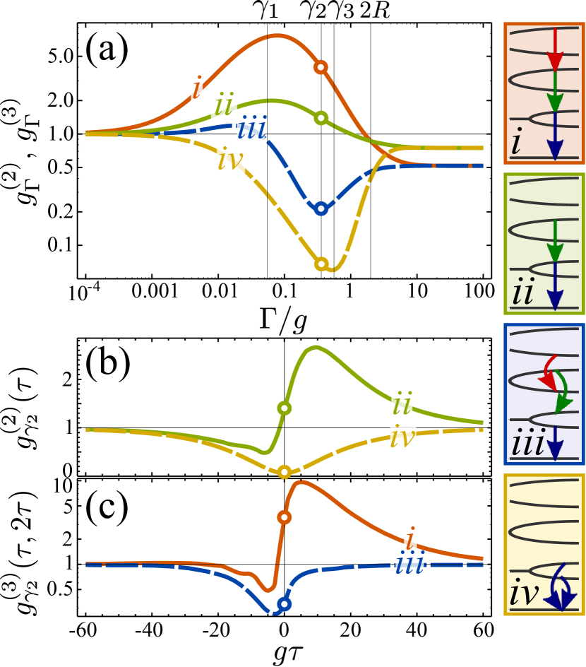
Figure 2: (Color online) (a) Two- and three-photon correlations at zero delay as a function of the sensor linewidth $\Gamma$, with frequencies of detection as shown in the insets $i$–$iv$. (b-c) $\tau$-dynamics of the correlation functions with $\Gamma=\gamma_{2}$ for, (b), two photons in the configurations of insets $ii$ and $iv$ and, (c), three photons in the configurations $i$ and $iii$. Positive $\tau$ corresponds to detection in the order from top to bottom of the ladder. Parameters: $P_{\sigma}=\gamma_{\sigma}=0.01g$, $\gamma_{a}=0.1g$.

In conclusion, we have presented a theory to efficiently compute correlations between an arbitrary number of photons of any given frequencies and time delays. All three aspects of the detection, namely frequencies, time-delays and linewidths of the detectors, are needed to characterise meaningfully the system. The method allows to compute exactly, with low effort and for general open quantum systems, properties of output fields that are otherwise defined in terms of complicated integrals. Its ease of use enabled us to present the first computation of three and four time-resolved and frequency-filtered correlation functions. Its application will allow the interpretation of experiments which are routinely implemented in the laboratory but which lacked hitherto an adequate and tractable theoretical support, and to design new ways to unravel and/or engineer the quantum dynamics of open systems.