On quantum mean-field models and their quantum annealing

Abstract

This paper deals with fully-connected mean-field models of quantum spins with $p$-body ferromagnetic interactions and a transverse field. For $p=2$ this corresponds to the quantum Curie-Weiss model (a special case of the Lipkin-Meshkov-Glick model) which exhibits a second-order phase transition, while for $p>2$ the transition is first order. We provide a refined analytical description both of the static and of the dynamic properties of these models. In particular we obtain analytically the exponential rate of decay of the gap at the first-order transition. We also study the slow annealing from the pure transverse field to the pure ferromagnet (and vice versa) and discuss the effect of the first-order transition and of the spinodal limit of metastability on the residual excitation energy, both for finite and exponentially divergent annealing times. In the quantum computation perspective this quantity would assess the efficiency of the quantum adiabatic procedure as an approximation algorithm.

I Introduction

Finding the minimum of a cost function defined on a discrete configuration space is the central task of combinatorial optimization. Depending on the problem considered (i.e. the shape of the cost function), there exists or not fast (running in polynomial time with respect to the number of variables) algorithms for classical computers that performs the minimization, as classified by the computational complexity theory GareyJohnson .

In more physical terms this problem corresponds to finding the groundstate of an Hamiltonian (cost function) depending on discrete degrees of freedom (spins). This analogy has suggested an optimization algorithm named simulated annealing sa , that proceeds through a stochastic exploration of the phase space, according to transition rules obeying the detailed balance condition for a positive temperature, which is slowly reduced from a very high value down to zero. In this way energy barriers can be jumped over through thermal fluctuations, the final state of the system is the equilibrium at zero temperature, hence concentrated in the sought-for minimum of the cost function. Provided with a quantum computer, that is a device that obeys the laws of quantum mechanics at the level of its computing units, one can follow a similar idea but with quantum fluctuations replacing the thermal ones; this strategy is known as quantum annealing qa_first ; qa , or quantum adiabatic algorithm qaa , see qa_review_santoro ; qa_book_das_chakrabarti for reviews. The control parameter that replaces the temperature allows to tune the relative strength of the potential energy (the cost function) and of the “kinetic energy” (for instance a transverse field for spins 1/2). The system is initially prepared in the groundstate of the latter, then evolves according to Schrödinger’s equation with an Hamiltonian that slowly interpolates between the kinetic and the potential energy. If this interpolation is sufficiently slow the system remains at all times in the instantaneous groundstate of the Hamiltonian, and in particular at the end of the evolution it is found in the desired minimum of the cost function.

To assess the efficiency of these algorithms one has to specify how slow the evolution of the control parameter has to be in order that the final state indeed corresponds to the groundstate. In the quantum setting, which shall be the focus of this article, this condition is provided by the quantum adiabatic theorem messiah76 which, roughly speaking, states that the interpolation time has to be larger that the inverse square of the minimal energy gap between the instantaneous groundstate and the first excited state encountered along the interpolation. It thus appears that quantum phase transitions sachdev , where the gap closes in the thermodynamic limit, constitute the bottleneck for the efficiency of the quantum annealing. First-order phase transitions, at which the gap is typically exponentially small in the system size, are in this respect worse than second-order transitions for which, at least in non-disordered systems, the gap is only polynomially small.

Random instances of combinatorial optimization problems provide useful benchmark ensembles of cost functions on which to test various algorithms random_sat . They have been the object of an intense research activity at the crossroad between computer science, mathematics and theoretical physics book_Marc_Andrea . Several phase transitions have been unveiled that affect the typical number and organization of their ground and excited states BiMoWe00 ; MePaZe02 ; pnas07 . More recently the tools that allowed the description of these transitions have been extended to take into account the additional effect of a transverse field on the corrugated random cost function cavity_first ; cavity_ours . First order phase transitions as a function of the interpolating transverse field have been observed in some models qXOR ; young10 ; this did not come as a surprise as it is a recurrent feature of mean-field quantum disordered systems that have been extensively studied Goldschmidt90 ; NiRi98 ; BiCu01 ; jorg08 .

Even if a first order transition in a given model means that the corresponding combinatorial optimization problem will only be solved exactly in a time exponentially large in the system size, many questions remain open at this point. First, one should try to compute the exponential rate of growth of the adiabatic time. Second, and maybe more importantly, one should investigate what is the final energy of an evolution that is too fast to respect the adiabaticity criterion (a question reminiscent of the Kibble-Zurek mechanism, see review_kz for a recent review). Besides its intrisic physical relevance, this point is also deeply related to important issues in computational complexity theory, namely hardness of approximation results book_vazirani . Indeed, for some combinatorial optimization problems (MAX-3-SAT for instance, or even MAX-3-XORSAT whose decision version is in P) it is not only difficult to compute the exact value of the minimum cost function, but even providing an approximate answer that is asymptotically more precise than taking the value of the function at a random point in the configuration space is also a difficult problem hastad01 . Hence a fast non-adiabatic evolution has a computational interest if one can find a good compromise between the evolution time and the residual energy. In the classical case hardness of approximation results are often obtained via the PCP theorem pcp . In the quantum complexity litterature a quantum analog of the PCP theorem has been conjectured in qpcp_conjecture . For recent works on the approximation algorithms in the quantum complexity setting we refer the readers to qpcp_hastings ; qapprox_kempe .

In this paper we shall investigate the annealing on non-adiabatic timescales for a class of ferromagnetic, non disordered, mean-field models of the fully-connected type, with $p$-spin interactions. These can of course not be considered as difficult optimization problems. However, despite their simplicity that allows for an analytical resolution, they exhibit some of the features expected also in more realistic optimization problems, and therefore constitute useful toy-models to study. The statics botet83 ; ViMoDu04 ; ribeiro06 ; ribeiro08 ; jorg10 ; FiDuVi11 ; SeNi12 and the dynamics, both for quantum annealings santoro08 ; solinas08 ; itin09_1 ; itin09_2 and for quantum quenches ViPaAs04 ; DaSeSeCh06 ; sciolla11 , of this kind of models have been largely studied. From a technical point of view these models are relatively simple because their mean-field character allows for a semi-classical treatment, the small parameter in this limit being the inverse of the size of the system (instead of $\hbar$ in usual semi-classical computations). In most of previous works this semi-classical limit has been achieved through the introduction of spin coherent-states ribeiro08 ; RiPa09 , or instantonic computations jorg10 . Here our treatment will have more of a WKB flavour, with the magnetization playing the role of a particle coordinate. Moreover most of these works dealed with second-order phase transitions, at the exception of jorg10 ; FiDuVi11 , which studied the statics of models with first-order transitions. The annealing dynamics of such models with first-order phase transition was not investigated before, to the best of our knowledge.

Let us now explain the structure of the paper. In Sec. II we introduce the definition of the models (II.1) and present their thermodynamic behavior and phase diagram (II.2). Section III contains our investigations on their static properties, at a refined level with respect to the thermodynamic quantities. As explained in a first part (Sec. III.1) of this section, their mean-field character induces strong symmetries that allow to decompose their spectrum in various disconnected sectors. We provide an ordering theorem between different sectors in Sec. III.2. In Sec. III.3 we discuss the qualitative features of the spectrum of the model, and point to the following parts of the text where they are quantitatively derived. The main technical result is established in Sec. III.4, where we show how to determine the eigenvectors, at the leading level in the thermodynamic limit. This is then applied to the computation of various quantities: the density of states inside one sector (Sec. III.5), the finite gap between levels away from transitions (Sec. III.6), and the exponentially small gaps in Sec. III.7. The latter part is divided according to the location of the quasi-degenerate levels in the spectrum, we consider in particular the exponentially small gap between the groundstate and the first excited state at a first-order transition in Sec. III.7.1, and the exponentially small gap between the two ferromagnetic phases for even $p$ in Sec. III.7.2. The dynamics of the models is studied in Sec. IV. After a precise definition of the annealing procedure in Sec. IV.1 we recall the basic mechanism of the Landau-Zener model in Sec. IV.2 and discuss the behavior of the dynamics that it suggests, in view of the properties of the spectrum derived previously. The actual results are presented in Sec. IV.4 (resp. Sec. IV.5) for annealing on exponentially large (resp. finite) timescales. A simplified model, introduced in Sec. IV.3, is also studied for comparison. We finally draw our conclusions in Sec. V. Some technical details are deferred to a series of Appendices.

II Definition and thermodynamic properties of the models

II.1 Definition

We shall consider Hamiltonians of interacting spins 1/2, acting on the Hilbert space spanned by $\{|\underline{\sigma}\rangle|\underline{\sigma}=(\sigma_{1},\dots,\sigma_{N})\in\{-1,+1\}^{N}\}$. We denote ${\widehat{\sigma}_{i}^{x}}$, ${\widehat{\sigma}_{i}^{y}}$ and ${\widehat{\sigma}_{i}^{z}}$ the Pauli matrices acting on the $i$-th spin, and recall that in this basis, ${\widehat{\sigma}_{i}^{z}}|\underline{\sigma}\rangle=\sigma_{i}|\underline{\sigma}\rangle$, ${\widehat{\sigma}_{i}^{x}}|\underline{\sigma}\rangle=|\underline{\sigma}^{(i)}\rangle$, where $\underline{\sigma}^{(i)}$ is the configuration obtained from $\underline{\sigma}$ by flipping the $i$-th spin. The transverse and longitudinal magnetization per spin operators are defined as follows :

$$\widehat{m}^{x}=\frac{1}{N}\sum_{i=1}^{N}{\widehat{\sigma}_{i}^{x}}\ ,\qquad\widehat{m}^{z}=\frac{1}{N}\sum_{i=1}^{N}{\widehat{\sigma}_{i}^{z}}\ .$$ (1)

The Hamiltonian of the fully-connected $p$-spin ferromagnet is usually defined as $-N(\widehat{m}^{z})^{p}-\Gamma N\widehat{m}^{x}$, i.e. with $p$-body interactions along the $z$ axis, and a transverse field $\Gamma$ along the $x$ axis. The dependency in $N$ is chosen to ensure the extensivity of the model in the thermodynamic limit. For future convenience we shall trade $\Gamma$ for a parameter $s\in[0,1]$ and define

$$\widehat{H}(s)=-Ns(\widehat{m}^{z})^{p}-N(1-s)\widehat{m}^{x}\ .$$ (2)

Up to a change of the energy scale these two definitions are equivalent, with the correspondance $\Gamma=\frac{1-s}{s}$. The two limits $s=0$ and $s=1$ corresponds to a pure transverse field and pure ferromagnetic interactions along $z$, respectively. The mean-field character of the model arises from the form of the interacting term, which depends on the total magnetization only. The $p=2$ case corresponds to the quantum Curie-Weiss model, which can also be viewed as the anisotropic version of the Lipkin-Meshkov-Glick (LMG) model LMG ; botet83 ; ribeiro08 (the general LMG model contains pair-wise interactions in the $y$ and $z$ directions). The case $p\geq 3$ was investigated in jorg10 , and generalized in FiDuVi11 to a model where both $\widehat{m}^{z}$ and $\widehat{m}^{x}$ are raised to arbitrary powers, and in SeNi12 with the addition of antiferromagnetic pairwise interactions. The methods and results developed in this paper for the model of Eq. (2) are easily extended to these generalizations, as sketched in the conclusions.

II.2 Thermodynamic properties

We shall first briefly explain how to compute the free-energy density of this model, in the thermodynamic limit, and discuss its phase diagram. Similar derivations can be found in cavity_ours ; jorg10 ; SeNi12 . For a rigorous treatment of such models we refer the reader to QCW_rigorous . The partition function at inverse temperature $\beta$ can be obtained by mapping the quantum problem to a classical one with one additional imaginary time direction. Using the Suzuki-Trotter formula to disentangle the two non-commuting terms in the Hamiltonian, and inserting representations of the identity between each of the ${N_{\rm s}}$ Suzuki-Trotter slices one indeed obtains:

$$Z(\beta,s)\equiv\textrm{Tr}\,e^{-\beta\widehat{H}(s)}=\lim_{{N_{\rm s}}\rightarrow\infty}\underset{\underline{\sigma}(1),\dots,\underline{\sigma}({N_{\rm s}})}{\sum}\prod_{\alpha=1}^{{N_{\rm s}}}\langle\underline{\sigma}(\alpha)|e^{\frac{\beta}{{N_{\rm s}}}sN(\widehat{m}^{z})^{p}}e^{\frac{\beta}{{N_{\rm s}}}(1-s)N\widehat{m}^{x}}|\underline{\sigma}(\alpha+1)\rangle\ .$$ (3)

In this expression $\underline{\sigma}(1),\dots,\underline{\sigma}({N_{\rm s}})$ are ${N_{\rm s}}$ Ising spin configurations, with periodic boundary conditions $\underline{\sigma}({N_{\rm s}}+1)=\underline{\sigma}(1)$. As $\widehat{m}^{z}$ is diagonal in the basis chosen one obtains

$$Z(\beta,s)=\lim_{{N_{\rm s}}\rightarrow\infty}\underset{\underline{\sigma}(1),\dots,\underline{\sigma}({N_{\rm s}})}{\sum}\prod_{\alpha=1}^{{N_{\rm s}}}e^{\frac{\beta}{{N_{\rm s}}}sN\left(\frac{1}{N}\sum_{i=1}^{N}\sigma_{i}(\alpha)\right)^{p}}\langle\underline{\sigma}(\alpha)|e^{\frac{\beta}{{N_{\rm s}}}(1-s)N\widehat{m}^{x}}|\underline{\sigma}(\alpha+1)\rangle\ .$$ (4)

Thanks to the mean-field character of the model one can reduce the problem to a single-site one by defining $m(\alpha)=\frac{1}{N}\sum_{i=1}^{N}\sigma_{i}(\alpha)$ and imposing this definition, for each $\alpha$, by an exponential representation of the Dirac distribution with conjugate parameter $\lambda(\alpha)$:

$$Z = \lim_{{N_{\rm s}}\rightarrow\infty}\int\prod_{\alpha=1}^{N_{s}}\frac{{\rm d}m(\alpha){\rm d}\lambda(\alpha)}{2\pi{N_{\rm s}}/(\beta N)}\,e^{\frac{\beta N}{N_{s}}\sum_{\alpha=1}^{N_{s}}(sm(\alpha)^{p}-\lambda(\alpha)m(\alpha))}\underset{\underline{\sigma}(1),\dots,\underline{\sigma}({N_{\rm s}})}{\sum}\prod_{\alpha=1}^{{N_{\rm s}}}\langle\underline{\sigma}(\alpha)|e^{\frac{\beta}{{N_{\rm s}}}\sum_{i=1}^{N}[\lambda(\alpha){\widehat{\sigma}_{i}^{z}}+(1-s){\widehat{\sigma}_{i}^{x}}]}|\underline{\sigma}(\alpha+1)\rangle$$ (5)

$$= \lim_{{N_{\rm s}}\rightarrow\infty}\int\prod_{\alpha=1}^{N_{s}}\frac{{\rm d}m(\alpha){\rm d}\lambda(\alpha)}{2\pi{N_{\rm s}}/(\beta N)}\,\exp\left[N\left(\frac{\beta}{N_{s}}\sum_{\alpha=1}^{N_{s}}(s\,m(\alpha)^{p}-\lambda(\alpha)m(\alpha))+\ln\,\textrm{Tr}\prod_{\alpha=1}^{N_{s}}e^{\frac{\beta}{{N_{\rm s}}}(\lambda(\alpha){\widehat{\sigma}^{z}}+(1-s){\widehat{\sigma}^{x}})}\right)\right]\ .$$

Making the natural assumption that the dominant contribution comes from values of $m(\alpha)$ and $\lambda(\alpha)$ that are constant in imaginary time and equal to $m,\lambda$ respectively, and evaluating the integral via the saddle-point method yields

$$f(\beta,s)\equiv\lim_{N\to\infty}-\frac{1}{\beta N}\ln Z(\beta,s)=\inf_{m}\underset{\lambda}{\text{ext}}\left[-s\,m^{p}+\lambda\,m-\frac{1}{\beta}\ln 2\cosh(\beta\sqrt{\lambda^{2}+(1-s)^{2}})\right]\ .$$ (6)

The stationarity conditions for this function of $(m,\lambda)$ are

$$\lambda=p\,s\,m^{p-1}\ ,\qquad m=\frac{\lambda}{\sqrt{\lambda^{2}+(1-s)^{2}}}\tanh(\beta\sqrt{\lambda^{2}+(1-s)^{2}})\ .$$ (7)

Note that an alternative derivation of this result consists in making a mean-field approximation $(\widehat{m}^{z})^{p}\to\langle\widehat{m}^{z}\rangle^{p}+p\langle\widehat{m}^{z}\rangle^{p-1}(\widehat{m}^{z}-\langle\widehat{m}^{z}\rangle)$ in the Hamiltonian and setting self-consistently the average value in the single-spin problem thus obtained BrMuTh66 ; WiViVeDu12 .

The various observables can be expressed in terms of the relevant critical point $(m_{*}(\beta,s),\lambda_{*}(\beta,s))$, in particular the longitudinal and transverse magnetization per spin read respectively

$$\langle\widehat{m}^{z}\rangle=m_{*}(\beta,s)\ ,\qquad\langle\widehat{m}^{x}\rangle=\frac{1-s}{\sqrt{\lambda_{*}(\beta,s)^{2}+(1-s)^{2}}}\tanh(\beta\sqrt{\lambda_{*}(\beta,s)^{2}+(1-s)^{2}})=\frac{1-s}{s}\frac{1}{p}m_{*}(\beta,s)^{2-p}\ .$$ (8)

These expressions are easily obtained by adding to the Hamiltonian appropriate fields conjugated to the observables and by deriving the variational free-energy with respect to these additional fields; the last expression of Eq. (8) is only valid under the assumption $m_{*}(\beta,s)\neq 0$.

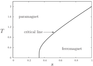
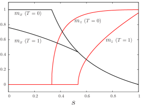
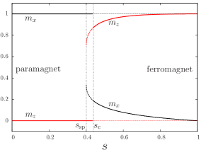
Let us first discuss the solution of these equations for $p=2$, and present the associated phase diagram. The point $(m,\lambda)=(0,0)$ is always a solution of Eq. (7). There is however a line in the $(s,\beta)$ plane separating a paramagnetic phase (at low values of $\beta,s$, i.e. high values of the temperature and transverse field) where it corresponds to the global minimum of the function in (6), from a ferromagnetic phase where it becomes a local maximum. In the latter phase there appears two global minima related by the symmetry operation $(m,\lambda)\to(-m,-\lambda)$. The spontaneous longitudinal magnetization $m_{*}(\beta,s)>0$ grows continuously from 0 at the border of the ferromagnetic phase, with the usual mean-field exponent $\beta=1/2$. The phase transition is thus of second order, the free-energy and its first derivatives being continuous at the transition. These properties are illustrated in Fig. 1.

             

Figure 1: Thermodynamic properties of the $p=2$ model. Left panel: phase diagram, the line indicates the value ${T_{\rm c}}(s)$ of the critical temperature for the second-order transition between the paramagnetic and the ferromagnetic phases. Center panel: longitudinal ($m_{z}$, red lines) and transverse ($m_{x}$, black lines) magnetizations as a function of $s$, for $T=1$ and $T=0$; in the ferromagnetic phase $m_{x}$ is independent of $T$, as apparent from the last expression of Eq. (8) with $p=2$. Right panel: free-energy density as a function of $s$ for $T=1$, and ground-state energy as a function of $s$; the arrows indicate the values $s_{\rm c}(T)$ of the transition between the paramagnet (black lines) and the ferromagnet (red lines).

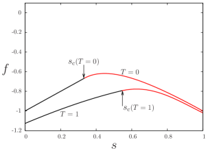
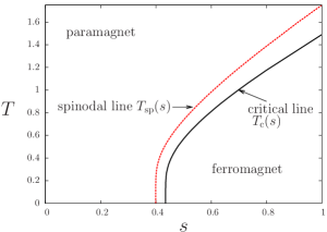
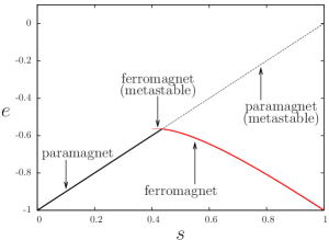
Consider now the case $p\geq 3$. The paramagnetic solution $(m,\lambda)=(0,0)$ of Eq. (7) is then a local minimum (with respect to $m$) of the function in (6) for all values of $(\beta,s)$. For low values of $\beta,s$ this is the only minimum of (6). Beyond a line $\beta_{\rm sp}(s)$ (or equivalently $s_{\rm sp}(\beta)$), another local minimum appears discontinuously in $m_{*}(\beta,s)>0$ (if $p\geq 4$ is even there is also a symmetric one in $-m_{*}(\beta,s)$). At its appearance this non-trivial local minimum corresponds to an higher free-energy density than the paramagnetic one. It is only for strictly larger values of $\beta,s$ than their free-energy density becomes equal, on the line $\beta_{\rm c}(s)>\beta_{\rm sp}(s)$ (or $s_{\rm c}(\beta)>s_{\rm sp}(\beta)$). The model thus exhibits a first-order phase transition along the line $\beta_{\rm c}(s)$, associated to a discontinuity in the first derivatives of the free-energy density, which implies in particular a discontinuity of the magnetizations. The line $\beta_{\rm sp}(s)$ is the spinodal of the ferromagnetic phase, i.e. the limit of its existence as a metastable local minimum of the free-energy. Note that the paramagnetic phase is always locally stable, there is thus no spinodal line for this phase. The features of this first-order transition are illustrated on Fig. 2; to anticipate the discussion of the rest of the paper the results displayed there are at zero temperature, yet they would be qualitatively identical at any positive temperature below the transition temperature of the classical model (at $s=1$).

             

Figure 2: Thermodynamic properties of the $p=3$ model (all cases with $p\geq 3$ are qualitatively identical). Left panel: phase diagram, the solid (black) line stands for the first-order transition line ${T_{\rm c}}(s)$, the dashed (red) line being the spinodal curve $T_{\rm sp}(s)$ for the limit of existence of the ferromagnetic phase. Center panel: longitudinal ($m_{z}$, red line) and transverse ($m_{x}$, black line) magnetizations as a function of $s$, at $T=0$. Solid thick part of the curves correspond to the thermodynamically relevant phase (paramagnetic for $s<s_{\rm c}$, ferromagnetic for $s>s_{\rm c}$), dashed light ones to the metastable ones ($s>s_{\rm c}$ for the metastable paramagnet, $s\in[s_{\rm sp},s_{\rm c}]$ for the metastable ferromagnet). Note the square-root singularity at $s_{\rm sp}$ for the magnetizations of the ferromagnetic phase. Right panel: groundstate energy density as a function of $s$; solid thick and dashed light have the same meaning as in the center panel.

In the remaining of this section we shall collect for future use some more explicit formulas valid in the zero-temperature limit, which will be the most useful case in the following of the paper. The groundstate energy density is obtained from (6) as

$$e_{\rm gs}(s)=\lim_{\beta\to\infty}f(\beta,s)=\inf_{m}\underset{\lambda}{\text{ext}}\left[-s\,m^{p}+\lambda\,m-\sqrt{\lambda^{2}+(1-s)^{2}}\right]\ .$$ (9)

One can solve explicitly the stationarity condition with respect to $\lambda$, which yields $\lambda=(1-s)m/\sqrt{1-m^{2}}$ and thus

$$e_{\rm gs}(s)=\inf_{m}\left[-s\,m^{p}-(1-s)\sqrt{1-m^{2}}\right]\ .$$ (10)

The energy corresponding to the paramagnetic state $m=0$ is $e_{\rm pm}(s)=-(1-s)$. For $p\geq 3$ the ferromagnetic phase exists when $s\in[s_{\rm sp},1]$, where $s_{\rm sp}$ is the zero-temperature limit of the spinodal line. We shall denote $m_{*}(s)>0$ the non-trivial solution of the stationarity equations corresponding to a local minimum for $s\in[s_{\rm sp},1]$, and $e_{\rm fm}(s)=-s\,m_{*}(s)^{p}-(1-s)\sqrt{1-m_{*}(s)^{2}}$ the corresponding energy. We also define $m_{\rm i}(s)$ and $e_{\rm i}(s)$ as the magnetization and energy of the local maximum (unstable phase of intermediate magnetization) of the function in (10). These magnetizations are the solutions, ordered with $0<m_{\rm i}(s)<m_{*}(s)$, of the equation

$$m=p\frac{s}{1-s}m^{p-1}\sqrt{1-m^{2}}\ .$$ (11)

The average magnetizations are then given by

$$\langle\widehat{m}^{z}\rangle=m_{*}(s)\ ,\qquad\langle\widehat{m}^{x}\rangle=\sqrt{1-m_{*}(s)^{2}}\ .$$ (12)

At the spinodal point we call $m_{\rm sp}=m_{*}(s_{\rm sp})=m_{\rm i}(s_{\rm sp})$ and $e_{\rm sp}=e_{\rm fm}(s_{\rm sp})=e_{\rm i}(s_{\rm sp})$ the longitudinal magnetization and the energy, while the first-order transition happens for $s_{\rm c}$ such that $e_{\rm pm}(s_{\rm c})=e_{\rm fm}(s_{\rm c})={e_{\rm c}}$, with ${m_{\rm c}}=m_{*}(s_{\rm c})$. Explicit formulas can be given for these quantities. Consider first the spinodal point. $m_{*}(s)$ is the solution of an implicit equation of the form $m=g(m,s)$, with the function $g$ defined by the r.h.s. of Eq. (11). The spinodal corresponds to a bifurcation of this implicit equation, in consequence $(m_{\rm sp},s_{\rm sp})$ are solutions of $m_{\rm sp}=g(m_{\rm sp},s_{\rm sp})$ and $1=\left.\frac{\partial g}{\partial m}\right|_{(m_{\rm sp},s_{\rm sp})}$. Solving this system yields

$$m_{\rm sp}=\sqrt{1-\frac{1}{p-1}}\ ,\qquad s_{\rm sp}=\frac{1}{1+p\frac{(p-2)^{(p-2)/2}}{(p-1)^{(p-1)/2}}}\ .$$ (13)

At the first-order transition point, the equation ${m_{\rm c}}=g({m_{\rm c}},s_{\rm c})$ is supplemented by the condition $e_{\rm pm}(s_{\rm c})=e_{\rm fm}(s_{\rm c})$, which leads to

$${m_{\rm c}}=\sqrt{\frac{p(p-2)}{(p-1)^{2}}}\ ,\qquad s_{\rm c}=\frac{1}{1+\frac{p}{p-1}\left(\frac{p(p-2)}{(p-1)^{2}}\right)^{\frac{p-2}{2}}}\ ,\qquad{e_{\rm c}}=-(1-s_{\rm c})\ .$$ (14)

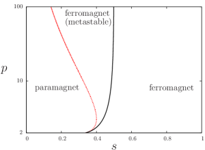
The dependency on $p$ of the spinodal and critical point parameters $s_{\rm sp}$ and $s_{\rm c}$ are plotted on Fig. 3. From the above explicit expressions one can in particular work out the large $p$ asymptotics, that read

$$m_{\rm sp}=1-\frac{1}{2p}+O(p^{-2})\ ,\quad s_{\rm sp}=\frac{e^{1/2}}{\sqrt{p}}+O(p^{-3/2})\ ,\quad{m_{\rm c}}=1-\frac{1}{2p^{2}}+O(p^{-3})\ ,\quad s_{\rm c}=\frac{1}{2}-\frac{1}{8p}+O(p^{-2})\ .$$ (15)

Figure 3: Spinodal line $s_{\rm sp}(p)$ and phase transition line $s_{\rm c}(p)$ in the $(s,p)$ plane, in logarithmic scale on the $p$ axis. For $p$ large, $s_{\rm c}\rightarrow 1/2$ whereas $s_{\rm sp}\rightarrow 0$ (the domain of existence of the metastable ferromagnetic phase grows with growing $p$).

III Detailed description of the spectrum

We shall now turn to a refined description of the statics of the model, beyond the computation of the thermodynamic limit of its free-energy density. This detailed study of the eigenvalues and eigenvectors of $\widehat{H}(s)$ will be crucial for the understanding of the annealing dynamics presented in Sec. IV. This section is organized as follows. In Sec. III.1 we exploit the symmetries of the model to decompose its Hilbert space into several disconnected sectors. In Sec. III.2 we prove a result on the relative ordering of the eigenvalues between different symmetry sectors, and provide a finer conjecture motivated by numerical evidences. The qualitative features of the spectrum inside one symmetry sector are discussed in Sec. III.3, and the rest of the section is devoted to the quantitative derivation of these properties. In Sec. III.4 we obtain the solution of the eigenvalue equation inside one sector, at the leading exponential level (in a semi-classical fashion). This main technical result is then exploited to obtain the density of states inside each sector (in Sec. III.5), the finite gaps between eigenvalues (in Sec. III.6) and the exponentially small gaps (in Sec. III.7), in particular at the first order transition of models with $p\geq 3$ (see Sec. III.7.1), and in the ferromagnetic phases for even $p$ (cf. Sec. III.7.2).

III.1 Decomposition of the Hilbert space in spin sectors

The diagonalization, be it numerical or analytical, of a quantum Hamiltonian is in general a very difficult task because of the exponential growth of the dimension of the Hilbert space with the size of the system. For the fully-connected mean-field models under study this difficulty is greatly reduced thanks to their highly symmetric structure: as a matter of fact the Hamiltonian is invariant under the permutation of any pair of spin indices.

Let us first briefly explain how to exploit this symmetry in an abstract and general way. The Hilbert space ${\cal H}$ of an $N$-component system is the tensorial product ${\cal H}=V^{\otimes N}$ of the space $V$ of each component. The theory of representation FultonHarris asserts that such a tensor product can be decomposed as a direct sum of vector spaces, classified according to their symmetry properties with respect to permutations. More precisely, in order to construct $V^{\otimes N}$ one has to sum over the Young diagrams with $N$ boxes and no more than $d$ rows, where $d$ is the dimension of $V$. Each of these diagrams gives rise to a Young symmetrizer, i.e. an operator on $V^{\otimes N}$ that, roughly speaking, completely symmetrizes along each row and antisymmetrizes along each column of the diagram. The tensor product $V^{\otimes N}$ can then be written as the direct sum of the images of the Young symmetrizers; the degeneracies in this sum, as well as the dimensions of these images, can be computed from the shape of the diagram. This decomposition can be useful only if the Hamiltonian itself respect such permutation symmetries, as it becomes block-diagonal once written in this basis.

This general theory that we only sketched above greatly simplifies in our case, and its consequences can be understood with more physical arguments. The important point is that the dimension $d$ of the base space of a spin $1/2$ is only $2$ here. In consequence the Young diagrams have at most two rows, and the sum over the diagrams reduces to a sum over the number $K=0,1,\dots,{\lfloor\frac{N}{2}\rfloor}$ of elements in the second row. This number counts the pair of spins over which the antisymmetrization procedure is accomplished. It can be given a more intuitive interpretation as follows. The operators ${\widehat{S}}^{\alpha}=\frac{N}{2}\widehat{m}^{\alpha}$ with $\alpha=x,y,z$ obey the commutation rules of an angular momentum; the total spin operator ${\widehat{S}}^{2}=({\widehat{S}^{x}})^{2}+({\widehat{S}^{y}})^{2}+({\widehat{S}^{z}})^{2}$ has thus eigenvalues of the form $S(S+1)$ with $S$ integer or half-integer. It turns out that the images of a Young symmetrizer with a given value of $K$ are eigenspaces of ${\widehat{S}}^{2}$, with total spin $S=\frac{N}{2}-K$. In particular the states of maximal spin $N/2$ correspond to fully symmetric states. More generally, the results of the abstract construction can be recovered by using recursively the standard rules for the addition of angular momenta.

Let us now summarize these results and write explicit formulas for the matrix elements of the Hamiltonian. There are

$${{\cal N}^{N}_{K}}=\binom{N}{K}\frac{N+1-2K}{N+1-K}=\binom{N}{K}-\binom{N}{K-1}$$ (16)

distinct eigenspaces of ${\widehat{S}}^{2}$ with spin $S=N/2-K$ (as could be expected the fully symmetric space $K=0$ is unique). Each of them has dimension $2S+1=N+1-2K$; using the second expression of ${{\cal N}^{N}_{K}}$ an easy computation allows to check that the total dimension of the Hilbert space is indeed

$$\sum_{K=0}^{\lfloor\frac{N}{2}\rfloor}{{\cal N}^{N}_{K}}(N+1-2K)=2^{N}\ .$$ (17)

The Hamiltonian $\widehat{H}(s)$ is stable with respect to this decomposition; moreover its action on one of these subspaces depends only on the value of $K$, not on the choice of one of the ${{\cal N}^{N}_{K}}$ degenerate sectors. We shall denote $\widehat{H}^{(K)}(s)$ the restriction of $\widehat{H}(s)$ to one of the subspaces of spin $N/2-K$, or equivalently view $\widehat{H}^{(K)}(s)$ as a square matrix of order $N+1-2K$. We will also use the notation $k=K/N$. The subspace on which $\widehat{H}^{(K)}(s)$ acts is spanned by the basis of eigenvectors of $\widehat{m}^{z}$, written $|m;K\rangle_{z}$ with the $N+1-2K$ possible values of $m$: ${{\cal M}^{N}_{K}}=\{-1+2k,-1+2k+2/N,\dots,1-2k-2/N,1-2k\}$. The action of $\widehat{m}^{x}$ on this vector amounts to increase or decrease the value of $m$ by its minimal amount $2/N$, i.e.

$$\phantom{}{}_{z}\langle m;K|\widehat{m}^{x}|m^{\prime};K\rangle_{z}=\frac{1}{2}\sqrt{(1-2k+\max(m,m^{\prime}))(1-2k-\min(m,m^{\prime}))}\quad\text{for}\ |m-m^{\prime}|=2/N\ .$$ (18)

The matrix representing $\widehat{H}^{(K)}(s)$ in this basis has thus a symmetric tridiagonal form, with matrix elements:

$$\phantom{}{}_{z}\langle m;K|\widehat{H}^{(K)}(s)|m;K\rangle_{z} = -N\,s\,m^{p}\ ,$$ (19)

$$\phantom{}{}_{z}\langle m;K|\widehat{H}^{(K)}(s)|m^{\prime};K\rangle_{z} = -N\frac{1-s}{2}\sqrt{(1-2k+\max(m,m^{\prime}))(1-2k-\min(m,m^{\prime}))}\quad\text{for}\ |m-m^{\prime}|=2/N\ .$$ (20)

One can also define a second basis spanned by the eigenvectors $|m;K\rangle_{x}$ of $\widehat{m}^{x}$. The expression of $\widehat{m}^{z}$ in this basis is nothing but Eq. (18) with the interversion of the indices $z$ and $x$. In this basis the matrix representation of $\widehat{H}^{(K)}(s)$ has a diagonal part corresponding to the action of the transverse field; the interaction term $(\widehat{m}^{z})^{p}$ has a band diagonal form, with non-zero matrix elements between eigenvectors $|m;K\rangle_{x}$ and $|m^{\prime};K\rangle_{x}$ when $\frac{N}{2}(m-m^{\prime})\in\{p,p-2,\dots,-p+2,-p\}$. We shall give and use their explicit form, in the large $N$ limit, in Sec. III.4.

These symmetry considerations thus allow to reduce the complexity of the full diagonalization of the Hamiltonian from a matrix problem of size $2^{N}$ to ${\lfloor\frac{N}{2}\rfloor}+1$ matrices of sizes at most $N+1$. This great simplification will be used in the following both for numerical and analytical computations.

The above reduction is valid for any model symmetric under all permutations of spins, irrespectively of the precise form of the interactions. The Hamiltonian of Eq. (2) exhibit additional symmetries:

• for odd values of $p$ the spectrum is invariant under the transformation $E\to-E$. Consider indeed an eigenvector $|\psi\rangle$ of $\widehat{H}^{(K)}(s)$, with eigenvalue $E$, written as $|\psi\rangle=\underset{m\in{{\cal M}^{N}_{K}}}{\sum}c_{m}|m;K\rangle_{z}$. Then the vector $|\psi^{\prime}\rangle=\underset{m\in{{\cal M}^{N}_{K}}}{\sum}c_{-m}(-1)^{\frac{N}{2}m}|m;K\rangle_{z}$ is an eigenvector of $\widehat{H}^{(K)}(s)$, with eigenvalue $-E$.

• for even values of $p$ the Hamiltonian is symmetric under global longitudinal magnetization reversal, and this implies that each $\widehat{H}^{(K)}(s)$ can be further decomposed in a block diagonal form, with two blocks of sizes ${\lfloor\frac{N}{2}\rfloor}+1-K$ and ${\lceil\frac{N}{2}\rceil}-K$. One can justify this statement in two ways. When acting on a basis vector $|m;K\rangle_{x}$, the operator $(\widehat{m}^{z})^{p}$, with $p$ even, produces a vector whose decomposition over $|m^{\prime};K\rangle_{x}$ is non-zero only for magnetizations $m^{\prime}$ such that $N/2(m-m^{\prime})$ is even: non-zero off-diagonal matrix elements in the $x$ basis are only found at an even distance from the main diagonal, hence in that basis the parity of the number of spin flips with respect to the fully polarized vector in the $x$ direction is conserved by the Hamiltonian.

  In addition, the matrix representing $\widehat{H}^{(K)}(s)$ in the $|m;K\rangle_{z}$ basis commutes with the matrix with 1 on the anti-diagonal (from bottom left to top right), that represents the reversal of the magnetization along the $z$ axis. The eigenvectors of $\widehat{H}^{(K)}(s)$ can thus be divided between those that are symmetric or antisymmetric under this transformation.

III.2 Ordering properties of the spectra

      

Figure 4: The eigenvalues $E_{i}^{(K)}(s)$ of the Hamiltonian $\widehat{H}(s)$, for $N=12$, $p=2$ (left) and $N=12$, $p=3$ (right). The different values of $K$ are distinguished by different colors and line styles.

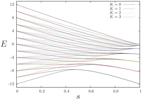
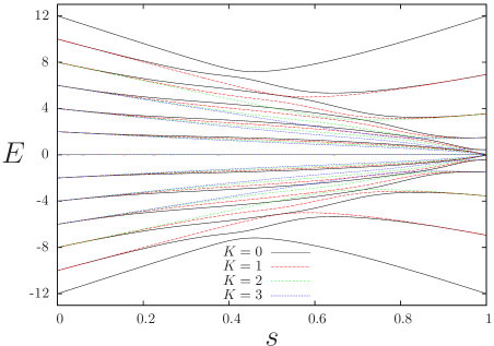
For each value of $K$ the restriction $\widehat{H}^{(K)}(s)$ of $\widehat{H}(s)$ to a subspace of spin $N/2-K$ has $N+1-2K$ real eigenvalues, that we shall denote $E_{0}^{(K)}(s)\leq E_{1}^{(K)}(s)\leq\dots\leq E_{N-2K}^{(K)}(s)$. We leave implicit the dependency of these quantities on $N$ and $p$, that are understood to be fixed in this whole subsection. By construction the Hamiltonian has no matrix elements between sectors of the Hilbert space corresponding to different values of $K$; one could thus a priori think that the spectrum $\{E_{i}^{(K)}(s)\}$ has no relationship to $\{E_{i}^{(K^{\prime})}(s)\}$ for $K\neq K^{\prime}$. A quick look at the numerical results displayed in Fig. 4 reveals on the contrary that there are strong ordering rules between the energy levels of different spin sectors, reminiscent of the Lieb-Mattis theorem for the antiferromagnetic Heisenberg model LiMa62 (see also NaSpSt04 for a more recent treatment of the ferromagnetic case). As a first step we shall prove that the groundstates of each sector are strictly ordered according to the spin of the sector, i.e. that

$$E_{0}^{(0)}(s)<E_{0}^{(1)}(s)<\dots E_{0}^{({\lfloor\frac{N}{2}\rfloor})}(s)\ \ \forall s\in[0,1]\ ,$$ (21)

in such a way that the global groundstate of $\widehat{H}(s)$ lies in the fully symmetric subspace $K=0$, of maximal spin $N/2$.

The proof goes as follows. Let us denote $|\psi\rangle$ the eigenvector of $\widehat{H}^{(K)}$ corresponding to its groundstate eigenvalue $E_{0}^{(K)}$, for some value of $K>0$. We decompose this vector on the basis in which $\widehat{m}^{z}$ is diagonal,

$$|\psi\rangle=\sum_{m\in{{\cal M}^{N}_{K}}}c_{m}|m;K\rangle_{z}\ .$$ (22)

We saw above that in this basis $\widehat{H}^{(K)}$ is a tri-diagonal matrix whose off-diagonal elements are all positive (cf. Eq. (20)). The Perron-Frobenius theorem thus ensures that the coefficients $c_{m}$ can be chosen to be all strictly positive. Let us now define a vector $|\psi^{\prime}\rangle$ belonging to the space on which $\widehat{H}^{(K-1)}$ acts, according to

$$|\psi^{\prime}\rangle=\sum_{m\in{{\cal M}^{N}_{K}}}c_{m}|m;K-1\rangle_{z}\ .$$ (23)

In a column representation this amounts to supplement $|\psi\rangle$ with two null rows corresponding to the two values $m=\pm(1-2k+2/N)$. This vector being normalized, the variational principle asserts that $E_{0}^{(K-1)}\leq\langle\psi^{\prime}|\widehat{H}^{(K-1)}|\psi^{\prime}\rangle$. One finds easily that

$$\langle\psi^{\prime}|\widehat{H}^{(K-1)}|\psi^{\prime}\rangle=E_{0}^{(K)}-N(1-s)\sum_{m\in{{\cal M}^{N}_{K}}\setminus 1-2k}c_{m}c_{m+\frac{2}{N}} \left[\sqrt{\left(1-2k+m+\frac{4}{N}\right)\left(1-2k-m+\frac{2}{N}\right)}\right.$$ (24)

$$\left.-\sqrt{\left(1-2k+m+\frac{2}{N}\right)\left(1-2k-m\right)}\right]\ .$$

The difference of the square roots being strictly positive, as well as the product $c_{m}c_{m+\frac{2}{N}}$, one thus obtains $E_{0}^{(K-1)}(s)<E_{0}^{(K)}(s)$ as long as $s<1$. On the other hand for $s=1$ the matrices are diagonal and the groundstate is obviously $E_{0}^{(K)}(s=1)=-N(1-2k)^{p}$, which also obeys the strict inequality $E_{0}^{(K-1)}(s=1)<E_{0}^{(K)}(s=1)$. This completes the proof of Eq. (21).

A closer look at the plots in Fig. 4 suggests that not only the groundstates are ordered between one sector and another, but also that excited states are interleaved in a regular way. For instance the first excited state of one sector, $E_{1}^{(K)}$, seems to always have a lower energy than the groundstate of the following sector, $E_{0}^{(K+1)}$. More generally, we propose the following conjecture based on this numerical investigation: for all $n\leq N/2$ if $p$ is odd, $n\leq N$ if $p$ is even, one has

$$E_{n}^{(0)}(s)<E_{n-1}^{(1)}(s)<\dots<E_{0}^{(n)}(s)\ \ \forall s\in(0,1)\ .$$ (25)

In particular, if this statement is true, the first excited state of the Hamiltonian $\widehat{H}(s)$ in the full Hilbert space is always in the sector of maximal spin. The consistency of this conjecture for $s$ close to $0$ and $1$ can easily be checked by perturbative expansions.

III.3 The salient features of the spectrum

In this section we describe qualitatively the main features of the spectrum of eigenstates in the symmetric sector of maximal spin (all sectors behaving in a similar way), that are apparent by visual inspection of the figures. We emphasize the connections with the thermodynamic computations of Sec. II.2, and also point to the following parts of the article where these properties are derived quantitatively.

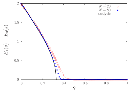
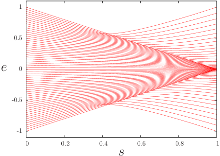
Let us begin with the $p=2$ case, for which the zero-temperature limit of the thermodynamic computation predicts a second-order phase transition at $s_{\rm c}=1/3$. The complete spectrum of the symmetric sector is plotted on the left panel of Fig. 5 for $N=60$. One observes indeed a good agreement with the shape of the groundstate energy predicted previously and plotted in the right panel of Fig. 1. Looking more carefully at the two states of lowest energy, one sees that the gap between them is of order 1 (in extensive energy $E=Ne$) in the paramagnetic phase (i.e. for $s<s_{\rm c}$), but exponentially small in $N$ in the ferromagnetic phase and indistinguishable in this figure. This exponentially small splitting is the consequence of the existence of the two magnetizations $\pm m_{*}(s)$ minimizing the thermodynamic groundstate energy (10). On the right panel of Fig. 5 we display the gap between the lowest states for two finite values of $N$, along with the analytical prediction of Eq. (52) for its limit when $N\to\infty$, that we shall obtain in Sec. III.5. The rate of the exponential splitting in the ferromagnetic phase will be derived in Sec. III.7.2, see Eq. (64) and right panel of Fig. 11. The square-root vanishing of the gap when $s\to s_{\rm c}^{-}$ and the behavior of the rate of exponential splitting when $s\to s_{\rm c}^{+}$ leads, with a finite-size scaling assumption explained in Sec. III.7.2, to a polynomial closing of the gap as $N^{-1/3}$ in the critical regime $s\approx s_{\rm c}$. This behaviour has been first predicted on the basis of the scaling analysis in botet83 ; the lifting of the degeneracy between ferromagnetic states was also studied in schulman76 . Note finally that the quasi-degeneracy of ferromagnetic states also occurs for excited eigenvalues: on the left panel of Fig. 5 one gets the impression that there are twice as less states on the right of a diagonal line $e=-(1-s)$ that on the left. This visual impression shall be confirmed in Sec. III.7.3.

      

Figure 5: Left panel: the spectrum of the symmetric sector of the $p=2$ model for $N=60$, obtained by numerical diagonalization. Right panel: the gap between the groundstate and the first excited state for $p=2$. The solid line is the result of an analytical computation, see Eq. (52), the symbols have been obtained by numerical diagonalization.

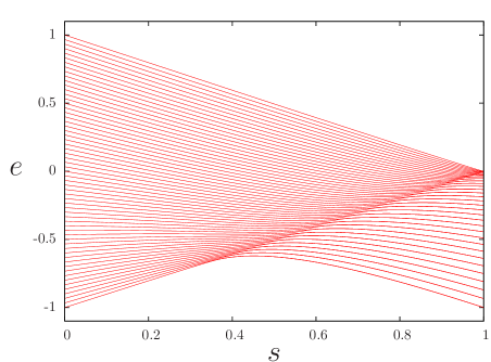
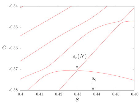
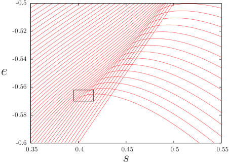
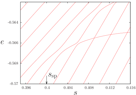
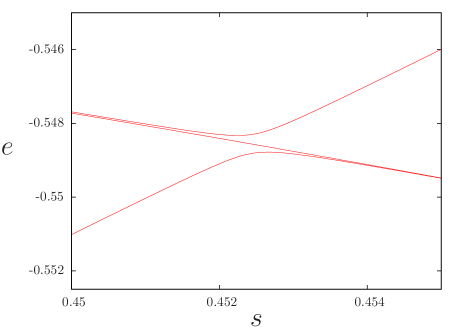
Let us now turn to the $p=3$ case, which has a first-order transition at $s_{\rm c}$. The spectrum of its maximal spin sector is displayed for $N=60$ on the left panel of Fig. 6. The slope of the groundstate energy is discontinuous at $s_{\rm c}$, as in the thermodynamic computation (compare with the right panel of Fig. 2). At variance with the $p=2$ case the gap between the groundstate and the first excited state remains of order 1 until one gets very close to $s_{\rm c}$; this is best seen on the right panel of Fig. 6, which displays a blow up of the lowest energy states around $s_{\rm c}$. The minimal gap (reached in $s_{\rm c}(N)$ which goes to $s_{\rm c}$ in the large $N$ limit) is indeed exponentially small at the first order transition; its exponential rate of decrease, which has been determined numerically and via an instantonic computation in jorg10 , will be computed in Sec. III.7.1 and given as an explicit analytic formula in Eq. (62). The level repulsion between the two lowest eigenstates is at work only in a small neighborhood of their point of avoided crossing, and it is tempting to infer from this plot that the first excited eigenvector for $s\gtrsim s_{\rm c}(N)$ is the continuation of the groundstate eigenvector of $s\lesssim s_{\rm c}(N)$ (and leads thus to the same thermodynamic observables), and vice versa. This pattern of avoided crossing looks actually very familiar, and can be observed in many examples involving the eigenvalues of an operator depending on an external parameter, $s$ here. Let us recall the fundamental reason behind the universality of such a pattern, and the justification of the continuation intuition (a detailed discussion of this point can be found in schulman76 ). The matrix elements of the operator $\widehat{H}(s)$ are analytic functions of $s$. As a consequence the eigenvalues $E_{i}^{(K)}(s)$ (in any symmetry sector $K$) are the roots of an algebraic (characteristic) equation of order $N+1-2K$, whose coefficients are analytic functions of $s$. Then one can prove (see for instance theorem XII.2 in reedsimon ) that the $E_{i}^{(K)}(s)$ are analytic functions of $s$, with at most algebraic branchpoint singularities at the (a priori complex) values of $s$ where the roots are degenerate. An avoided crossing is thus due to the two eigenvalues being strictly equal when an infinitesimally small imaginary part is added to $s$. By performing the interpolation between $s\lesssim s_{\rm c}(N)$ and $s\gtrsim s_{\rm c}(N)$ via a detour in the complex plane avoiding the branchpoint singularity one can thus define in a precise way the first excited eigenvector on one side of the avoided crossing as the analytic continuation of the groundstate on the other side. The thermodynamic calculations of Sec. II.2 suggest that the paramagnetic state of energy $e=-(1-s)$ is metastable for all values $s\in[s_{\rm c},1]$, and indeed one observes on the plots of Fig. 6 and 7 a continuation of this eigenstate across a series of avoided crossings. On the contrary the ferromagnetic state which corresponds to the groundstate for $s\geq s_{\rm c}$ only exists down to a spinodal point $s_{\rm sp}$, beyond which the analytic continuation cannot be performed anymore. This is illustrated on the two panels of Fig. 7. The exponential rate of closing of the gaps encountered along the continuation of the paramagnetic and ferromagnetic state shall be computed analytically in Sec. III.7.4, along with a determination of the area in the $(s,e)$ plane where avoided crossings do occur (see Sec. III.7.3).

All odd values of $p\geq 3$ yield behaviors similar to the $p=3$ case. The models with an even value of $p\geq 4$ exhibit both the first-order phenomenology of the $p=3$ case and the exponentially small splitting between the two ferromagnetic states allowed by the spin-flip symmetry. This shall be further discussed in Sec. III.7.2 and Sec. III.7.3.

      

Figure 6: Left panel: the spectrum of the symmetric sector of the $p=3$ model for $N=60$, obtained by numerical diagonalization. Right panel: a zoom on the lowest energy part of the spectrum around the avoided crossing between the lowest energy eigenstates at $s_{\rm c}(N)$. In the thermodynamic limit the first-order transition occurs at $s=s_{\rm c}$.

      

Figure 7: Left panel: a part of the spectrum for $p=3$, with $N=320$, in the neighborhood of the spinodal point of the ferromagnetic phase. Right panel: a zoom on the area of the black box of the left panel. All the crossings are actually avoided, but some of the gaps are too small to be distinguished on the picture.

III.4 The semi-classical solution of the eigenvalue equation

We shall now determine the structure of the eigenvectors of $\widehat{H}(s)$, in the thermodynamic limit $N\to\infty$, with a calculation formally similar to the WKB semi-classical treatment of quantum mechanics, the size of the system $N$ playing the role of $\hbar^{-1}$. Similar semi-classical analysis have been performed for mean-field spin models in ulyanov92 ; ribeiro08 ; RiPa09 using a spin-coherent-state representation; at variance with these works we shall use here the eigenbasis of $\widehat{m}^{z}$ or $\widehat{m}^{x}$.

As explained above this computation amounts to diagonalize the matrices of order $N+1-2K$ representing the restriction $\widehat{H}^{(K)}(s)$ to a sector of spin $N/2-K$. For simplicity, and because this will be the most useful case in the following, we shall concentrate here on the fully symmetric $K=0$ situation. The generalization to higher values of $K$ is straightforward and sketched in Sec. III.5. Let us look for an eigenvector $|\phi(s,e)\rangle$ of $\widehat{H}^{(0)}(s)$ with eigenvalue $Ne$, written in the $z$-diagonal basis as

$$|\phi(s,e)\rangle=\sum_{m\in{{\cal M}^{N}_{0}}}\phi(m,s,e)\,|m;0\rangle_{z}\ .$$ (26)

Using the expression of the matrix elements given in Eqs. (19,20), one obtains the equation obeyed by the coefficients $\phi(m,s,e)$:

$$e\,\phi(m,s,e)=-s\,m^{p}\,\phi(m,s,e) - \frac{(1-s)}{2}\sqrt{1-m^{2}+\frac{2}{N}(1-m)}\ \phi\left(m+\frac{2}{N},s,e\right)$$ (27)

$$- \frac{(1-s)}{2}\sqrt{1-m^{2}+\frac{2}{N}(1+m)}\ \phi\left(m-\frac{2}{N},s,e\right)\ .$$

To deal with the $N\to\infty$ limit we shall make the following Ansatz on the behaviour of the eigenvector components: $\phi(m,s,e)=e^{-N\varphi(m,s,e)}$, with $\varphi(m,s,e)$ an a priori smooth complex function. Then $\phi(m+2/N,s,e)+\phi(m-2/N,s,e)=2\phi(m,s,e)\cosh\left(2\varphi^{\prime}(m,s,e)+O(1/N)\right)$, where ^′ denotes the derivative with respect to $m$, and (27) can be rewritten, at the leading order, as:

$$e=-s\,m^{p}-(1-s)\sqrt{1-m^{2}}\,\cosh\left(2\varphi^{\prime}(m,s,e)\right)\ .$$ (28)

Inverting this relation yields

$$\varphi^{\prime}(m,s,e)=\frac{1}{2}\arg\cosh\left(-\frac{e+s\,m^{p}}{(1-s)\sqrt{1-m^{2}}}\right)\ ,$$ (29)

the analog of the eikonal equation in the semi-classical one-dimensional quantum mechanics context. Several points have to be precised for this equation to unambiguously determine the eigenvector rate function $\varphi(m,s,e)$. First of all, not all values of $e$ should correspond to an authorized eigenvalue of the Hamiltonian. Then the value of $\varphi$ has to be fixed at one point $m$ to reconstruct $\varphi$ from its derivative. Finally $\arg\cosh$ is a multi-valued function, hence one should precise which of its branches to use.

These ambiguities are actually solved by imposing that $\phi$ is normalizable in the large $N$ limit, and that $\varphi^{\prime}$ is continuous in $m$ (the coefficients of the eigenvalue equation (27) being smooth in $m$). By fixing for instance the norm of $\phi$ to be of order 1, the first requirement imposes that $\underset{m}{\inf}[\Re\,\varphi(m,s,e)]=0$ (we denote $\Re\,z$ and $\Im\,z$ the real and imaginary part of $z$). To precise the meaning of the $\arg\cosh$ function let us first define the functions $\text{ach}\,(t)$ as the reciprocal of $\cosh$ that maps the interval $t\in[1,\infty)$ to $[0,\infty)$, and $\text{acos}\,(t)$ the reciprocal of $\cos$ that maps $t\in[-1,1]$ to $[0,\pi]$. Then, as the argument of the $\arg\cosh$ in Eq. (29) is always real, it is enough to define

$$\arg\cosh t=\begin{cases}i\pi\pm\text{ach}\,(-t)&\text{if}\ t\leq-1\\ i\,\text{acos}\,(t)&\text{if}\ t\in[-1,1]\\ \pm\text{ach}\,(t)&\text{if}\ t\geq 1\end{cases}\ .$$ (30)

There are two branchpoints in $\pm 1$, where the function thus defined is continuous independently of the choice of the sign of its real part.

Let us now derive from these considerations the authorized value of the eigenvalue (per spin) $e$. Notice first that the argument of $\arg\cosh$ in Eq. (29) diverges in $m\to\pm 1$, hence it cannot be confined to $[-1,1]$ for all values of $m\in[-1,1]$. There remains two cases to consider: either the argument crosses at least once one of the two branch-points $\pm 1$, or it remains larger (in absolute value) than 1 for all $m$. In the latter case one cannot change branch and the sign of the real part of $\varphi^{\prime}$ is constant on $m\in[-1,1]$ (otherwise $\varphi^{\prime}$ is not continuous), hence one cannot fulfill the condition $\underset{m}{\inf}[\Re\,\varphi(m,s,e)]=0$ in a non-trivial way. A moment of thought reveals that on the contrary in the former case one can construct a normalizable eigenvector. This implies that the range of authorized values for $e$ is

$$\underset{m\in[-1,1]}{\text{Image}\,}[-s\,m^{p}-(1-s)\sqrt{1-m^{2}}]\cup\underset{m\in[-1,1]}{\text{Image}\,}[-s\,m^{p}+(1-s)\sqrt{1-m^{2}}]\ .$$ (31)

In particular the groundstate energy, for a given value of $s$, is obtained from this reasoning as

$$e_{\rm gs}(s)=\inf_{m\in[-1,1]}\left[-s\,m^{p}-(1-s)\sqrt{1-m^{2}}\right]\ ,$$ (32)

in perfect agreement with the thermodynamic computation of Sec. II.2, see Eq. (10).

In the following sections III.5, III.7.1 and III.7.2 we shall show explicitly, in various cases, how to choose the correct branches of the $\arg\cosh$ function when crossing a branchpoint and how to determine the rate function $\varphi(m,s,e)$ by integration of Eq. (29). A particularly important issue will be the occurence of multiple valid eigenvectors corresponding, at the leading order, to the same eigenvalue $e$. Before that we shall present a very simple example to check the above computation, and an alternative formulation in another basis.

A simple consistency check of Eq. (29) can be performed for $s=0$, i.e. in a pure transverse field. In that case it is easy to see that for all $N$ the groundstate has energy $-N$, with the eigenvector

$$|\phi(s=0,e=-1)\rangle=\frac{1}{2^{N/2}}\sum_{m\in{{\cal M}^{N}_{0}}}\sqrt{\binom{N}{N\frac{1+m}{2}}}|m;0\rangle_{z}\ ,$$ (33)

corresponding to all spins aligned in the $x$ direction. These values of $\phi(m,s=0,e=-1)$ solve exactly Eq. (27); with the help of the Stirling formula one obtains the value of $\varphi$ in the $N\to\infty$ limit,

$$\varphi_{0}(m)\equiv\varphi(m,s=0,e=-1)=\frac{1+m}{4}\ln(1+m)+\frac{1-m}{4}\ln(1-m)\ .$$ (34)

Let us now check that the computation presented above gives back this result. We have from Eq. (29)

$$\varphi^{\prime}(m,s=0,e=-1)=\frac{1}{2}\arg\cosh\left(\frac{1}{\sqrt{1-m^{2}}}\right)\ .$$ (35)

The argument of the $\arg\cosh$ reaches the branchpoint 1 only in $m=0$. To enforce the condition $\underset{m}{\inf}[\Re\,\varphi(m,s,e)]=0$ one has to choose the branches as

$$\varphi^{\prime}(m,s=0,e=-1)=\text{sign}\,(m)\frac{1}{2}\text{ach}\,\left(\frac{1}{\sqrt{1-m^{2}}}\right)\ ,$$ (36)

hence upon integration with the boundary condition $\varphi(m=0,s=0,e=-1)=0$,

$$\varphi(m,s=0,e=-1)=\frac{1}{2}\int_{0}^{m}\text{sign}\,(m)\,\text{ach}\,\left(\frac{1}{\sqrt{1-m^{\prime 2}}}\right){\rm d}m^{\prime}=\frac{1}{2}\int_{0}^{m}\arg\tanh(m^{\prime}){\rm d}m^{\prime}=\frac{1}{4}\int_{0}^{m}\ln\left(\frac{1+m^{\prime}}{1-m^{\prime}}\right){\rm d}m^{\prime}\ ,$$ (37)

in agreement with the direct computation yielding (34).

We shall finally present a similar computation of the eigenvectors of $\widehat{H}^{(0)}(s)$, but using now the $x$ basis, namely we write

$$|\phi(s,e)\rangle=\sum_{m\in{{\cal M}^{N}_{0}}}\phi_{x}(m,s,e)\,|m;0\rangle_{x}\ .$$ (38)

The coefficients $\phi_{x}$ obey the following equation (the equivalent of Eq. (27) in the $z$ basis):

$$e\,\phi_{x}(m,s,e)=-(1-s)\,m\,\phi_{x}(m,s,e)-s\left(\frac{1-m^{2}}{4}\right)^{p/2}\sum_{u=0}^{p}\binom{p}{u}\,\phi_{x}\left(m+\frac{2}{N}(p-2u),s,e\right)\ ,$$ (39)

in which we have dropped some irrelevant terms of order $1/N$. As above we look for a solution of this equation under the form $\phi_{x}(m,s,e)=e^{-N\varphi_{x}(m,s,e)}$, and find that the leading behaviour of $\varphi_{x}$ is ruled by the equation

$$e = -(1-s)m-s\left(\frac{1-m^{2}}{4}\right)^{p/2}\sum_{u=0}^{p}\binom{p}{u}(e^{2\varphi_{x}^{\prime}(m,s,e)})^{p-u}(e^{-2\varphi_{x}^{\prime}(m,s,e)})^{u}$$ (40)

$$= -(1-s)m-s(1-m^{2})^{p/2}\cosh(2\varphi_{x}^{\prime}(m,s,e))^{p}\ .$$ (41)

This yields finally the equivalent of Eq. (29):

$$\varphi_{x}^{\prime}(m,s,e)=\frac{1}{2}\arg\cosh\left(\left(-\frac{e+(1-s)m}{s(1-m^{2})^{\frac{p}{2}}}\right)^{1/p}\right)\ .$$ (42)

This equation suffers from the same kind of ambiguities as Eq. (29), the $p$-th root and the $\arg\cosh$ function being multi-valued. However these ambiguities can also be solved with exactly the same reasoning as the one following Eq. (29). In most of the paper we shall use the $z$-basis computation; the use of the $x$-basis will however reveal useful in Sec. IV.5.2.

III.5 The computation of the density of states inside one symmetry sector

We shall now present the first application of the above computation of the eigenvectors, that will give an explicit formula for the integrated density of eigenvalues (similar results for the LMG model can be found in ribeiro08 ). Let us first define this notion precisely, and emphasize its difference with another, maybe more usual, related concept. The full Hilbert space of the model (2) is $2^{N}$ dimensional, and its “density of states” can be defined as the microcanonical entropy $\sigma(s,e)$, such that $e^{N\sigma(s,e)}{\rm d}e$ gives, at the leading order, the number of eigenvalues of (2) in the interval $[Ne,N(e+{\rm d}e)]$. This quantity is obtained from the free-energy density (6) via a Legendre transform between $e$ and $\beta$. In this section we shall however investigate a finer quantity, namely the density of eigenvalues for the restriction $\widehat{H}^{(K)}$ of the Hamiltonian to one symmetry sector (which has $N+1-2K$ eigenvalues). Consider for instance the fully-symmetric sector, and define

$${\cal D}_{0}(s,e)=\underset{N\to\infty}{\lim}\frac{1}{N+1}|\{j|E^{(0)}_{j}(s)\leq Ne\}|$$ (43)

as the integrated density of states inside that sector. We shall see at the end of this section that the knowledge of the integrated density of states of all sectors $K=0,\dots,{\lfloor\frac{N}{2}\rfloor}$ provides a much more detailed information on the system than the microcanonical entropy.

There is actually a simple relation between ${\cal D}_{0}(e,s)$ and the leading order computation of the eigenvectors of the previous Subsection, based on the following observation: $\widehat{H}^{(K)}$, expressed in the $z$-basis, is a symmetric tridiagonal matrix with all elements next to the diagonal of the same sign (negative). This implies that the ordering in energies of its eigenvalues corresponds to the number of nodes of the associated eigenstates, exactly for the same reasons as the $n$-th excited eigenstate of a one-dimensional quantum particle described by the Schrödinger equation has precisely $n$ zeroes. A proof for the discrete case can be adapted from the usual reasonings in the Schrödinger case (see derrida93 for a similar derivation in another context), and shows that the groundstate of $\widehat{H}^{(K)}$ is a Perron-Frobenius vector whose elements can be taken all positive, while its first excited state presents exactly one “domain wall” between two sets of values of $m$ where the eigenvector is positive/negative, and so on and so forth. As we defined $\phi(m)=e^{-N\varphi(m)}$, the fact that excited eigenstates exhibit alternating signs translates into $\varphi$ acquiring an imaginary part. More precisely, each “domain wall” between opposite signs for $\phi(m)$ corresponds to an increase of its phase by $\pm\pi$. One can thus count the number of nodal points of $\phi$ by integrating the imaginary part of $\varphi^{\prime}$ on $m\in[-1,1]$, and deduce from it the number of eigenvalues that have lower energies. This reasoning yields the following formula,

$${\cal D}_{0}(s,e)=\frac{1}{\pi}\int_{-1}^{1}{\rm d}m\,\Im\,\varphi^{\prime}(m,s,e)\ ,$$ (44)

as we have chosen in Eq. (30) a branch of $\arg\cosh$ with positive imaginary part. Using the value (29) for the derivative of $\varphi$ one obtains a completely explicit formula for the integrated density of states in the maximal spin sector,

$$\begin{split}{\cal D}_{0}(s,e)=\frac{1}{2\pi}\int_{-1}^{1}{\rm d}m\,\left[\text{acos}\,\left(-\frac{e+s\,m^{p}}{(1-s)\sqrt{1-m^{2}}}\right)\mathbb{I}\left(-\frac{e+s\,m^{p}}{(1-s)\sqrt{1-m^{2}}}\in[-1,1]\right)\right.\\ \left.+\pi\,\mathbb{I}\left(-\frac{e+s\,m^{p}}{(1-s)\sqrt{1-m^{2}}}\leq-1\right)\right]\ ,\end{split}$$ (45)

where we defined $\mathbb{I}(A)$ to be $1$ if $A$ is true, $0$ otherwise. Deriving this expression with respect to $e$ one can equivalently obtain an expression for the density of states,

$$\rho_{0}(s,e)=\frac{1}{2\pi}\int_{-1}^{1}{\rm d}m\,\left[\frac{1}{\sqrt{(1-s)^{2}(1-m^{2})-(e+s\,m^{p})^{2}}}\mathbb{I}\left(-\frac{e+s\,m^{p}}{(1-s)\sqrt{1-m^{2}}}\in[-1,1]\right)\right]\ .$$ (46)

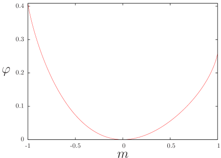
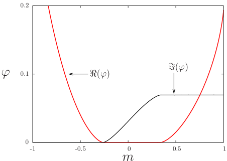
We give in Fig. 8 some examples of the construction of $\varphi$, for $p=3$ and $s=0.3$, i.e. in the paramagnetic phase. For the ground-state energy $e=-(1-s)$ the argument of the $\arg\cosh$ function in Eq. (29) is always $\geq 1$, with a single point of equality in $m=0$. As a consequence the corresponding solution for $\varphi$ is everywhere real, see left panel of the figure. On the contrary for a slightly higher value of the energy ($e=e_{\rm gs}+0.1$ on the figure) the branchpoint $1$ is crossed at two values of $m$, hence the imaginary part of $\varphi$ grows on this interval, on which the real part vanishes identically.

      

Figure 8: Plots of the eigenstate function $\varphi$, for $p=3$ and $s=0.3$. Left panel: for the groundstate energy, $e=e_{\rm gs}$, $\varphi$ is purely real. Right panel, for a slightly larger energy, $e=e_{\rm gs}+0.1$, $\varphi$ acquires an imaginary part.

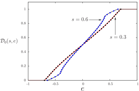
We also present on Fig. 9 the curves for the integrated density of states ${\cal D}_{0}$ for $p=3$ and two values of $s$, $0.3$ and $0.6$ (in the latter case one observes a singularity at the crossing of the energy of the metastable paramagnetic phase). The agreement with the density of states obtained by numerical diagonalization is very good already for small values of $N$ ($N=40$ on the figure).

Figure 9: Plots of the integrated density of states ${\cal D}_{0}$ for $p=3$, $s=0.3$ and $s=0.6$. The solid lines are our analytical predictions from Eq. (45); the symbols are the results of numerical diagonalization of systems with $N=40$.

Let us briefly mention here one application of this computation that shall be useful in the analysis of the annealing dynamics. From the integrated density of states ${\cal D}_{0}(s,e)$ one can define “iso-integrated density lines” $e_{\rm iso}(s)$ by imposing that ${\cal D}_{0}(s,e_{\rm iso}(s))$ remains constant when $s$ is varied. These lines correspond to the thermodynamic limit of the energy density of some (excited) eigenvalues, as long as no level crossings occurs.

We shall now explain how to generalize the computation of the integrated density of states to sectors of arbitrary spin $N/2-K$. The matrix of size $N+1-2K$ representing the restriction $\widehat{H}^{(K)}$ of the Hamiltonian to this sector has matrix elements given in Eqs. (19,20). Denoting $k=K/N$, one can look for eigenstates of $\widehat{H}^{(K)}$ under the form $e^{-N\varphi(m,s,e)}$, where the longitudinal magnetization $m$ is now restricted to $[-1+2k,1-2k]$, and the function $\varphi$ is solution of a generalization of Eq. (29), namely

$$\varphi^{\prime}(m,s,e)=\frac{1}{2}\arg\cosh\left(-\frac{e+s\,m^{p}}{(1-s)\sqrt{(1-2k)^{2}-m^{2}}}\right)\ .$$ (47)

The rest of the computation follows strictly the reasoning made for the symmetric ($K=0$) sector. In particular the groundstate energy density for a sector with $k=K/N$ reads in the thermodynamic limit

$$e_{\rm gs}^{(k)}(s)=\inf_{m\in[-1+2k,1-2k]}\left[-s\,m^{p}-(1-s)\sqrt{(1-2k)^{2}-m^{2}}\right]\ ,$$ (48)

and the density of states in that sector is

$$\begin{split}{\cal D}_{k}(s,e)=\frac{1}{2\pi}\int_{-1+2k}^{1-2k}{\rm d}m\,\left[\text{acos}\,\left(-\frac{e+s\,m^{p}}{(1-s)\sqrt{(1-2k)^{2}-m^{2}}}\right)\mathbb{I}\left(-\frac{e+s\,m^{p}}{(1-s)\sqrt{(1-2k)^{2}-m^{2}}}\in[-1,1]\right)\right.\\ \left.+\pi\,\mathbb{I}\left(-\frac{e+s\,m^{p}}{(1-s)\sqrt{(1-2k)^{2}-m^{2}}}\leq-1\right)\right]\ .\end{split}$$ (49)

We shall finaly compare the amount of information contained in the densities of states ${\cal D}_{k}(s,e)$ on one hand, and the microcanonical entropy $\sigma(s,e)$ on the other. The latter being the Legendre transform of the free-energy, we shall equivalently discuss this quantity. Using the decomposition of the Hilbert space into symmetry sectors the partition function can be written as

$$Z=\sum_{K=0}^{{\lfloor\frac{N}{2}\rfloor}}{{\cal N}^{N}_{K}}\sum_{j=0}^{N-2K}e^{-\beta E_{j}^{(K)}}\ ,$$ (50)

where ${{\cal N}^{N}_{K}}$ gives the number of degenerate representations of spin $N/2-K$ (see Eq. (16)), and $E_{j}^{(K)}$ is the $j$-th eigenvalue of $\widehat{H}^{(K)}$. In the thermodynamic limit the degeneracy ${{\cal N}^{N}_{K}}$ grows exponentially with $N$; on the contrary the sum over the eigenstates of one sector contains only a linear number of terms, and is thus dominated at the leading exponential order by the greatest of these terms, i.e. the groundstate energy of the corresponding sector. This leads to the following expression for the free-energy density,

$$f(\beta,s)=\inf_{k\in[0,1/2]}\left[e_{\rm gs}^{(k)}(s)-\frac{1}{\beta}(-k\ln k-(1-k)\ln(1-k))\right]\ .$$ (51)

A short computation based on the expression of $e_{\rm gs}^{(k)}$ given in (48) reveals the agreement between this expression and the one obtained in Sec. II.2 (see Eq. (6)). What we want to stress here is that the only “microscopic” (i.e. at the level of eigenstates) input of the computation is the energy density of the groundstate in each sector. The microcanonical entropy is thus entirely dominated by the effect of the degeneracy ${{\cal N}^{N}_{K}}$ of the various spin sectors, and is completely insensitive to their internal structure beyond their groundstate energy density.

III.6 The computation of finite gaps

One can estimate the energy gaps between eigenvalues from the density of states obtained in Eq. (46): in the interval $[e,e+{\rm d}e]$ of (intensive) energy one finds $N\rho(s,e){\rm d}e$ eigenvalues. Assuming these levels to be equispaced, the gap between two successive eigenvalues is, in extensive energy, $1/\rho(s,e)$ ribeiro08 . This computation can be performed in any part of the energy spectrum; for simplicity we shall only state some results, obtained by combining this observation with the explicit expressions of the density of states (46) and of its integrated form (45), in the most relevant regions of the spectrum.

For $p=2$, i.e. in the Curie-Weiss model, one obtains in the paramagnetic phase ($s<s_{\rm c}$) for the gap between the groundstate and the first excited state:

$$\lim_{N\to\infty}[E^{(0)}_{1}(s)-E^{(0)}_{0}(s)]=\frac{1}{\rho(s,e_{\rm gs}(s))}=2\sqrt{3}\sqrt{(1-s)(s_{\rm c}-s)}\ ,$$ (52)

as found in botet83 , and plotted on the right panel of Fig. 5. Note the square-root closing of the gap at the second-order transition. The same computation performed in the ferromagnetic phase ($s>s_{\rm c}$) yields

$$\frac{1}{\rho(s,e_{\rm gs}(s))}=\sqrt{3}\sqrt{(1+s)(s-s_{\rm c})}\ .$$ (53)

This should however not be interpreted as the gap between the first two eigenvalues, but rather as half the gap between the groundstate and the second excited state. Indeed the level splitting between the two lowest states is exponentially small in $N$ (as will be computed in Sec. III.7.2) and the density of states does not distinguish them. In other words the hypothesis of equi-spacing of eigenvalues is strongly broken in this situation.

Consider now the case $p>2$. In the paramagnetic phase ($s\leq s_{\rm c}$) one finds

$$\lim_{N\to\infty}[E^{(0)}_{1}(s)-E^{(0)}_{0}(s)]=\frac{1}{\rho(s,e_{\rm gs}(s))}=2(1-s)$$ (54)

for the gap between the two lowest levels, which is the same result as would have been obtained if the Hamiltonian contained only the transverse field term. Note also that the gap thus computed remains positive at the first-order transition; the exponentially small gap (to be determined in Sec. III.7.1) cannot be detected by the density of states. The computation of the density of states $\rho_{0}$ at the groundstate energy can similarly be performed in the ferromagnetic phase (i.e. for $s\geq s_{\rm c}$). For odd values of $p$ one finds

$$\underset{N\to\infty}{\lim}[E^{(0)}_{1}(s)-E^{(0)}_{0}(s)]=\frac{1}{\rho(s,e_{\rm gs}(s))}=2psm_{*}(s)^{p-2}\sqrt{(p-1)m_{*}(s)^{2}-(p-2)}\ ,$$ (55)

which is positive at $s_{\rm c}$. For even values of $p$ this computation, as explained above in the case $p=2$, gives an information only on the gap between the groundstate and the second excited state. After a short computation one obtains a similar formula,

$$\underset{N\to\infty}{\lim}[E^{(0)}_{2}(s)-E^{(0)}_{0}(s)]=\frac{2}{\rho(s,e_{\rm gs}(s))}=2psm_{*}(s)^{p-2}\sqrt{(p-1)m_{*}(s)^{2}-(p-2)}\ ;$$ (56)

one could expect to find an additional factor $2$ in this expression with respect to the odd $p$ case, however this factor compensates because of the contributions of the two minima in $\pm m_{*}(s)$ in the density of states ${\cal D}_{0}$.

For $p>2$ a richer behaviour is displayed in the neighborhood of the spinodal point of coordinates $(s_{\rm sp},e_{\rm sp})$. In particular in the limit $s\to s_{\rm sp}^{-}$ one finds after some computations a scaling behaviour for the integrated density of states, of the form

$${\cal D}_{0}(s_{\rm sp}-\delta s,e_{\rm sp}+\delta e)-{\cal D}_{0}(s_{\rm sp},e_{\rm sp})\sim\delta s\,\mathcal{G}((\delta e+e^{\prime}_{\rm fm}(s_{\rm sp})\delta s)\delta s^{-6/5})\ ,$$ (57)

where $e^{\prime}_{\rm fm}(s_{\rm sp})=-m_{\rm sp}^{p}+\sqrt{1-m_{\rm sp}^{2}}$ is the derivative of the energy of the ferromagnetic metastable state at the spinodal. The scaling function $\mathcal{G}(z)$ is monotonously increasing, behaves as $|z|^{5/6}$ for $|z|\to\infty$, and vanishes in one point we shall denote $z_{0}$. The iso-integrated density line that goes through the spinodal point behaves thus as $e_{\rm iso}(s_{\rm sp}-\delta s)\sim-e^{\prime}_{\rm fm}(s_{\rm sp})\delta s+z_{0}\delta s^{6/5}$. Moreover in the scaling regime the density of states can be obtained by deriving the above relation, namely

$$\rho_{0}(s_{\rm sp}-\delta s,e_{\rm sp}+\delta e)\sim\delta s^{-1/5}\,\mathcal{G}^{\prime}((\delta e+e^{\prime}_{\rm fm}(s_{\rm sp})\delta s)\delta s^{-6/5})\ .$$ (58)

In consequence the finite gap between the eigenstate level that reaches the spinodal point and the first excited state above it closes when $s\to s_{\rm sp}^{-}$ as $\delta s^{1/5}/\mathcal{G}^{\prime}(z_{0})$. This fifth root is to be contrasted with the square root singularity for the groundstate of $p=2$. Moreover we should warn the reader that the correction $z_{0}\delta s^{6/5}$ in the expansion of the eigenstate energy is crucial: in $z=0$ the scaling function $\mathcal{G}$ is finite but has no derivative, and the expansion of $\rho_{0}$ without taking into account the correction leads to $\rho_{0}(s_{\rm sp}-\delta s,e_{\rm sp}-e^{\prime}_{\rm fm}(s_{\rm sp})\delta s)\propto\delta s^{-1/4}$, which modifies the exponent from $1/5$ to $1/4$.

III.7 The computation of exponentially small gaps

As discussed qualitatively in Sec. III.3 the energy gaps between two successive levels are, in some regions of the plane $(s,e)$ depending on $p$, exponentially small in the size $N$ of the system. This section is devoted to the computation of the exponential rate of closing of those gaps. It is divided in four parts; we shall first investigate the avoided crossing between the groundstate and the first excited state at the first-order transition of the models with $p\geq 3$ (in Sec. III.7.1), then compute the exponentially small splitting between the two lowest levels in the ferromagnetic phase of even $p$ models (in Sec. III.7.2). The next two subsections will be devoted to exponentially small gaps between excited states; in Sec. III.7.3 we shall determine the values of $(s,e)$ where these avoided crossings do occur, and in Sec. III.7.4 we will concentrate on the avoided crossings encountered by the metastable continuations of the paramagnetic and ferromagnetic groundstates.

From a technical point of view the common pattern behind the appearance of an exponentially small gap is the existence of two valid solutions of the semi-classical eigenvalue equation (29) for the same value of $e$. This approximate degeneracy is lifted at the exponential order, the splitting between the two levels being proportional to the exponentially small scalar product between the two quasi-eigenvectors computed at leading order. This can be shown by writing the eigenvalue equation in the two dimensional Hilbert space spanned by the two quasi-eigenvectors. In more physical terms this corresponds to the semi-classical approximation of quantum mechanics for a double-well potential, in which the two lowest energy levels have a gap exponentially small in $1/\hbar$.

III.7.1 The exponentially small gap at the first order transition for $p\geq 3$

The first case we shall consider is the exponentially small gap between the groundstate and the first excited state at the first-order transition for $p\geq 3$. We first concentrate on the odd $p$ case for simplicity, the modifications to be made when $p$ is even are discussed afterwards.

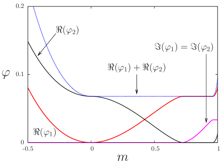
From the thermodynamic considerations of Sec. II.2 we showed that this transition happens at a ($p$-dependent) value of $s$ denoted $s_{\rm c}$, where the infimum in the definition (10) of the groundstate energy is reached for two distinct values of $m$, i.e. in $m=0$ and $m={m_{\rm c}}>0$ (see Eq. (14) for the values of $s_{\rm c}$ and ${m_{\rm c}}$). The paramagnetic and ferromagnetic phases have thus the same energy ${e_{\rm c}}$. In terms of the eigenstate computation, this observation translates into the fact that the argument of the $\arg\cosh$ in the expression of $\varphi^{\prime}(m,s_{\rm c},{e_{\rm c}})$ given by (29) is $\geq 1$ for all values of $m$, with two point of equalities in $m=0$ and $m={m_{\rm c}}$. The prescription for the choices of the branches of the $\arg\cosh$ function (that can be changed at the branching point $+1$) explained after Eq. (29) leaves us with two possible real solutions $\varphi_{1}$ and $\varphi_{2}$, which reaches their minimal value $0$ in $m=0$ and $m={m_{\rm c}}$ respectively. These two functions are plotted for $p=3$ in Fig. 10.

Figure 10: The two possible eigenstate functions $\varphi_{1,2}(m,s_{\rm c},{e_{\rm c}})$ at the first order transition point of the $p=3$ model.

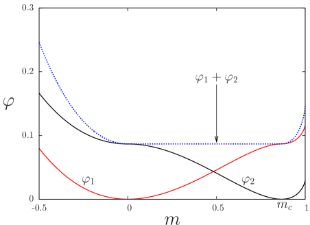
This apparent degeneracy of the lowest eigenvalues is however lifted with an exponentially small correction in $N$. Let us denote $\alpha_{p}$ the rate at which this gap closes with $N$, i.e.

$$\alpha_{p}=-\lim_{N\to\infty}\frac{1}{N}\ln\left(\underset{s\in[0,1]}{\min}[E_{1}^{(0)}(s)-E_{0}^{(0)}(s)]\right)\ .$$ (59)

At leading order this rate can be computed from the overlap between the two quasi-eigenvectors $\phi_{1}(m)=e^{-N\varphi_{1}(m)}$ and $\phi_{2}(m)=e^{-N\varphi_{2}(m)}$, as explained at the beginning of this section. We thus have

$$\alpha_{p} = -\lim_{N\to\infty}\frac{1}{N}\ln|\langle\phi_{1}|\phi_{2}\rangle|=-\lim_{N\to\infty}\frac{1}{N}\ln\left|\int_{-1}^{1}{\rm d}m\,e^{-N\varphi_{1}(m,s_{\rm c},{e_{\rm c}})-N\varphi_{2}(m,s_{\rm c},{e_{\rm c}})}\right|$$ (60)

$$= \inf_{m}[\varphi_{1}(m,s_{\rm c},{e_{\rm c}})+\varphi_{2}(m,s_{\rm c},{e_{\rm c}})]\ .$$ (61)

The shape of the sum $\varphi_{1}+\varphi_{2}$ is also displayed in Fig. 10. It is minimal and constant on the whole interval $[0,{m_{\rm c}}]$; indeed the two functions are solutions of Eq. (29) for the same value of the parameters $e,s$, and only differ in the opposite choice of the branch of the $\arg\cosh$ function for their derivative on $[0,{m_{\rm c}}]$. As a consequence $\alpha_{p}$ can be simply computed by integrating the derivative of $\varphi$, i.e.

$$\alpha_{p}=\frac{1}{2}\int_{0}^{{m_{\rm c}}}{\rm d}m\ \text{ach}\,\left(-\frac{{e_{\rm c}}+s_{\rm c}\,m^{p}}{(1-s_{\rm c})\sqrt{1-m^{2}}}\right)\ .$$ (62)

This formula, complemented by the values of ${m_{\rm c}}$, $s_{\rm c}$ and ${e_{\rm c}}$ as a function of $p$ given in (14), is one of the main results of the statics part of the paper, giving a very explicit analytical prediction of the exponentially small gap at the first-order transition.

The numerical values of $\alpha_{p}$ thus obtained are displayed in Table 1, along with a comparison with the data reported by Jörg et al in jorg10 . The authors of this paper obtained $\alpha_{p}$ both by exact diagonalization of the matrices $\widehat{H}^{(0)}$ for finite $N$ (with an extrapolation in the limit $N\to\infty$) and by a semi-classical instantonic computation. Our results agrees very well with theirs. One can set up an asymptotic expansion of $\alpha_{p}$ at large $p$, that results in

$$\alpha_{p}=\frac{\ln 2}{2}-\frac{\pi^{2}}{12p}+O\left(\frac{1}{p^{2}}\right)\ ,$$ (63)

as stated in the Table. The details of this computation are deferred to Appendix A. The interpretation of $\alpha_{p}$ for even values of $p$ shall be discussed in the next section.

$p$	$\Gamma_{\rm c}$	$s_{\rm c}$	${m_{\rm c}}$	$\frac{\alpha_{p}}{\ln 2}$ (diagonalization) jorg10	$\frac{\alpha_{p}}{\ln 2}$ (instanton) jorg10	$\frac{\alpha_{p}}{\ln 2}$ from Eq. (62)
3	1.2991	0.4350	0.8660	0.126(3)	0.1251	0.1252
4	1.1852	0.4576	0.9428	-	-	0.2127
5	1.1347	0.4685	0.9682	0.270(3)	0.2686	0.2680
6	1.1059	0.4749	0.9798	-	-	0.3057
7	1.0873	0.4791	0.9860	0.335(3)	0.3335	0.3329
8	1.0743	0.4821	0.9897	-	-	0.3535
9	1.0647	0.4843	0.9922	0.370(3)	0.3699	0.3695
13	1.0426	0.4896	0.9965	0.410(3)	0.4105	0.4093
17	1.0318	0.4922	0.9980	0.431(3)	0.4315	0.4306
21	1.0253	0.4937	0.9987	0.445(3)	0.4445	0.4437
31	1.0168	0.4958	0.9994	0.462(3)	0.4623	0.4618
$p\to\infty$	$1+\frac{1}{2p}$	$\frac{1}{2}-\frac{1}{8p}$	$1-\frac{1}{2p^{2}}$	$\frac{1}{2}-\frac{1.15}{p}$	-	$\frac{1}{2}-\frac{\pi^{2}}{12\log 2}\frac{1}{p}$

Table 1: Exponential rate of decay of the gap between the groundstate and the first excited state at the first-order transition for the $p$-spin model, divided by $\ln 2$ to ease the comparison with the results of jorg10 . The last column is our result, computed from Eq. (62). The fifth column is the extrapolation from finite $N$ exact diagonalization jorg10 , and the sixth one results from an instantonic computation jorg10 . Thermodynamic parameters $\Gamma_{\rm c}=(1-s_{\rm c})/s_{\rm c}$, $s_{\rm c}$ and ${m_{\rm c}}$ of the system at the critical point are also given. The last line gives an equivalent of these quantities at the leading order in $1/p$ in the large $p$ limit.

III.7.2 The exponentially small gap between the two ferromagnetic phases for even $p$

For even values of $p$ the classical part of the Hamiltonian, $\widehat{H}(s=1)$, is invariant under the reversal of the longitudinal magnetization, its groundstate is thus doubly degenerate, with eigenstates fully polarized along the $\pm z$ direction. As soon as the transverse field is switched on, i.e. for $s<1$, this strict degeneracy is lifted. However in the ferromagnetic phase, i.e. for $s>s_{\rm c}$, this lifting is weak, and the gap between the groundstate and the first excited state is exponentially small in $N$, of the form $e^{-N\beta_{p}(s)}$ at the leading order. We shall now compute this rate $\beta_{p}(s)$, following essentially the same lines as in Sec. III.7.1. A similar study for $p=2$ can be found in schulman76 .

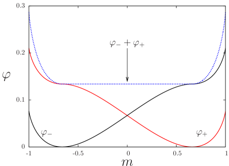
In the ferromagnetic phase of even $p$ models the infimum in the definition (10) of the groundstate energy is reached in $\pm m_{*}(s)$, where the spontaneous longitudinal magnetization $m_{*}(s)$ is solution of Eq. (11). Hence the argument of $\arg\cosh$ in Eq. (29) is $\geq 1$ for all values of $m$, touching 1 in $\pm m_{*}(s)$. One can thus construct two solutions $\varphi_{\pm}$ of Eq. (29), that vanish in $\pm m_{*}(s)$. An example for $p=2$ is displayed in Fig. 11. As above one obtains the rate $\beta_{p}(s)$ by computing the overlap between these two quasi-eigenstates. This yields

$$\beta_{p}(s)=\frac{1}{2}\int_{-m_{*}(s)}^{m_{*}(s)}{\rm d}m\,\text{ach}\,\left(-\frac{e_{\rm gs}(s)+s\,m^{p}}{(1-s)\sqrt{1-m^{2}}}\right)\ .$$ (64)

This formula compares very well with the results of exact diagonalization for $p=2$ florent_p2 , as shown in the right panel of Fig. 11.

      

Figure 11: Left panel: the two eigenstate functions $\varphi_{\pm}$ for $s=0.4$ and $p=2$, at the groundstate energy, and their sum. Right panel: exponential scaling of the gap $\beta_{2}(s)$ between the two ferromagnetic solutions for $p=2$. The solid black curve has been obtained from Eq. (64), the symbols are the results of exact diagonalization extrapolated in the limit $N\to\infty$ florent_p2 , the red dashed curve is the leading term in the $s\to 1$ limit, see Eq. (67).

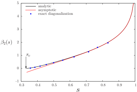
In the classical limit $s\to 1$ the gap vanishes for all values of $N$, in consequence the rate $\beta_{p}(s)$ diverges in this limit. One can study this asymptotic behavior more precisely. One has $m_{*}(s)\to 1$ and $e_{\rm gs}(s)\to-1$ in this limit, and the factor $1/(1-s)$ makes the argument of the ach  function in (64) diverge for all values of $m$ inside the domain of integration. One can then use the asymptotic expansion $\text{ach}\,(y)\sim\ln(2y)+o(1)$ for $y$ large to obtain

$$\beta_{p}(s)\sim\frac{1}{2}\int_{-1}^{1}{\rm d}m\,\ln\left(\frac{2}{1-s}\frac{1-m^{p}}{\sqrt{1-m^{2}}}\right)\sim-\ln(1-s)+\widehat{\beta}_{p}\ ,$$ (65)

where the constant $\widehat{\beta}_{p}$ can be expressed in terms of the harmonic number function $H(x)=\int_{0}^{1}\frac{1-t^{x}}{1-t}{\rm d}t$, as

$$\widehat{\beta}_{p}=\int_{0}^{1}{\rm d}m\,\ln\left(\frac{2(1-m^{p})}{\sqrt{1-m^{2}}}\right)=\ln 2-H\left(\frac{1}{p}\right)+\frac{1}{2}H\left(\frac{1}{2}\right)\ .$$ (66)

In particular for $p=2$ we obtain

$$\beta_{2}(s)\sim-\ln(1-s)-1+2\ln 2\ ,$$ (67)

which is also plotted for comparison in the right panel of Fig. 11.

Another interesting limit case concerns the behaviour of $\beta_{2}(s)$ around the threshold $s_{\rm c}$ of the second-order transition of the $p=2$ model. The rate of exponentially small splitting has to vanish in this limit, since the groundstate of the paramagnetic phase is no longer quasi-degenerate. More precisely, using the asymptotic behaviors $m_{*}(s)\sim 3\sqrt{s-s_{\rm c}}$ when $s\to s_{\rm c}^{+}$ and $\text{ach}\,(1+y)\sim\sqrt{2y}$ when $y\to 0^{+}$, one can expand the expression (64) of $\beta_{2}(s)$ and obtain after a short computation that $\beta_{2}(s)=9(s-s_{\rm c})^{3/2}+O((s-s_{\rm c})^{5/2})$. This exponent $3/2$ was first predicted in botet83 on the basis of an adaptation of Finite Size Scaling to mean-field systems (and found also in dusuel04 from the scaling of singular finite $N$ corrections). The argument of botet83 leads indeed to the value $\nu_{\rm mf}d_{\rm c}$, where $\nu_{\rm mf}$ and $d_{\rm c}$ are the mean-field value of the exponent controlling the divergence of the correlation length and the upper critical dimension of the universality class to which the studied model belongs. In the present case $\nu_{\rm mf}=1/2$, as in the $\phi^{4}$ theory, but one has to take $d_{\rm c}=3$: classical models in this universality class have an upper critical dimension of $4$, however in the Suzuki-Trotter formulation a $d$-dimensional quantum model is mapped onto a classical model with an additional imaginary time dimension of length $\beta$, and thus correspond to a $d+1$-dimensional classical model in the zero temperature limit. From this value of the exponent and the behavior of the gap in the paramagnetic phase (see Eq. (52)) the authors of botet83 could deduce the scaling with $N$ of the gap in the critical regime $s\approx s_{\rm c}$. Let us reproduce here their argument. Suppose that the gap $E_{1}(s)-E_{0}(s)$ satisfies a scaling assumption in the double limit $N\to\infty$, $s\to s_{\rm c}$, i.e.

$$E_{1}(s)-E_{0}(s)\sim N^{-x}\mathcal{F}((s-s_{\rm c})N^{x^{\prime}})\ ,$$ (68)

with $\mathcal{F}$ a scaling function and $x,x^{\prime}$ two exponents to be determined. This assumption can agree with the study of the ferromagnetic phase only if $x^{\prime}=2/3$, with $\mathcal{F}(z)\approx\exp[-9z^{3/2}]$ as $z\to+\infty$. On the other hand, approaching the transition from the paramagnetic phase leads to a closing of the (finite) gap as a square root (see Eq. (52)), hence $\mathcal{F}(z)\sim 2\sqrt{2}(-z)^{1/2}$ as $z\to-\infty$ and $x=x^{\prime}/2=1/3$. The scaling assumption and the behavior of the gap as $N^{-1/3}$ in the critical regime of the $p=2$ model were checked numerically in botet83 .

Let us finally discuss the structure of the gaps between the lowest states of a model with $p\geq 4$ even, in the neighborhood of its first-order transition. For the choice of parameters $(s,e)=(s_{\rm c},{e_{\rm c}})$, the argument of the $\arg\cosh$ function in Eq. (29) reaches the branching point $1$ in $-{m_{\rm c}},0$ and $+{m_{\rm c}}$, one can thus construct three distinct quasi-eigenvectors with rate $\varphi(m)$ vanishing for these three magnetizations. One could think that the reasoning presented at the beginning of this section, that reduces to the diagonalization of a two by two matrix, is invalidated. This is however not the case, as is best understood by looking at the three lowest levels of the $p=4$ model plotted on Fig. 12. On the ferromagnetic side of the transition the groundstate (resp. the first excited state) is the symmetric (resp. antisymmetric) combination of the ferromagnetic quasi-eigenvectors concentrated on $\pm{m_{\rm c}}$, with an exponentially small splitting of order $\exp[-N\beta_{p}(s_{\rm c})]$, while the second excited state is the metastable continuation of the paramagnetic groundstate. The avoided crossing of order $\exp[-N\alpha_{p}]$ thus occurs between the groundstate and the second excited state; as $\alpha_{p}=\frac{1}{2}\beta_{p}(s_{\rm c})$, this gap is much more opened than the one between the ferromagnetic states. The fact that the first excited state has no level repulsion at the avoided crossing is easily understood from the additional symmetry of even $p$ models discussed at the end of Sec. III.1: the paramagnetic and symmetric combination of ferromagnetic states belongs to the sector invariant with respect to the reversal of the longitudinal magnetization, while the antisymmetric combination is in the other, disconnected, sector. Note that on the paramagnetic side of the transition the splitting of order $\exp[-N\beta_{p}(s_{\rm c})]$ occurs between the first and second excited states.

Figure 12: The energy of the three lowest levels of the $p=4$ model in the neighborhood of the first-order transition, obtained from numerical diagonalization with $N=40$.

III.7.3 Exponentially small gaps between excited states

In the two previous cases we computed the exponentially small splitting between two quasi-degenerate groundstates, the ferromagnetic and paramagnetic ones at the first-order transition in Sec. III.7.1 and the two ferromagnetic ones in Sec. III.7.2. It should however be clear (see for instance the left panel of Fig. 7) that exponentially small gaps occur not only between the two lowest eigenstates, but also between excited ones. In this subsection we shall explain how to adapt the computation in that case, and in the next one we will in particular obtain the exponential rate of closing of the gaps encountered by the metastable continuation of the ferromagnetic and paramagnetic phases, which shall be a crucial ingredient for the analysis of the annealing dynamics in Sec. IV.

In terms of the leading order eigenvalue equation (29), an exponentially small splitting between two eigenstates shows up as the existence of two distinct solutions $\varphi_{1,2}(m,s,e)$ of Eq. (29) that both fulfill the condition $\underset{m}{\inf}[\Re\,\varphi(m,s,e)]=0$. We shall call $\gamma(s,e)$ the rate at which this gap closes, i.e. it is at the leading order of the form $e^{-N\gamma(s,e)}$. As previously explained this rate is obtained from the scalar product between the two quasi-eigenvectors. The two functions $\varphi_{1,2}$ only differ by a choice of branch of the $\arg\cosh$ function on an interval $[m_{1}(s,e),m_{2}(s,e)]$. This implies that their imaginary part is the same for all $m$ (see Eq. (30)), hence the scalar product between the two eigenvectors depends only on the real part of $\varphi_{1,2}$. This leads to:

$$\begin{split}\gamma(s,e)&=-\lim_{N\to\infty}\frac{1}{N}\ln|\langle\phi_{1}|\phi_{2}\rangle|=-\lim_{N\to\infty}\frac{1}{N}\ln\left|\int_{-1}^{1}{\rm d}m\,e^{-N\varphi^{*}_{1}(m,s,e)-N\varphi_{2}(m,s,e)}\right|\\ &=\inf_{m}\Re[\varphi_{1}(m,s,e)+\varphi_{2}(m,s,e)]=\frac{1}{2}\int_{m_{1}(s,e)}^{m_{2}(s,e)}{\rm d}m\,\text{ach}\,\left(\frac{|e+s\,m^{p}|}{(1-s)\sqrt{1-m^{2}}}\right)\ .\end{split}$$ (69)

Let us now describe the regions in the $(s,e)$ plane where exponentially small gaps occur. The discussion above shows that their occurence can be traced back to the number of times the argument of the $\arg\cosh$ function in Eq. (29) reaches the branching points $\pm 1$, in other words the number of solutions $m\in[-1,1]$ of the equations

$$e=-s\,m^{p}-(1-s)\sqrt{1-m^{2}}\qquad\text{or}\ \ e=-s\,m^{p}+(1-s)\sqrt{1-m^{2}}\ .$$ (70)

A moment of thought reveals that for any value of $(e,s)$ in the authorized range of eigenvalues (defined in (31)) this number is either 2, 4 or 6 (counting twice the marginal case of a branching point touched quadratically and not crossed). The first case corresponds to a non-degenerate eigenstate, the two others to exponentially small gaps between eigenstates. The frontiers between these domains correspond to the disappearance of some solutions of the equations (70), which define implicitly $m$ as a function of $s,e$. Their boundary can thus be obtained as the limits of validity of the implicit function theorem. After a short computation one realizes that they are given by curves $e(s)$ of the form (70), with $m$ replaced by one of the solutions (stable or instable) of Eq. (11). Let us be more concrete by distinguishing between various cases:

• for $p=2$, when $s\leq s_{\rm c}$ the spectrum is made of non-degenerate eigenvalues with $e\in[-(1-s),(1-s)]$. When $s\geq s_{\rm c}$ the low-energy part of the spectrum ($e\in[e_{\rm gs}(s),-(1-s)]$) has doubly degenerate eigenvalues with an exponentially small gap between them, while the high-energy spectrum ($e\in[-(1-s),1-s]$) is non-degenerate. These two regimes are depicted in the left panel of Fig. 13, and agree with the qualitative features described in Sec. III.3 on the basis of the numerical diagonalization (cf. the left panel of Fig. 5). For clarity a zoom of the latter is presented on the right panel of Fig. 13, in the neighborhood of the line $e=-(1-s)$, which is indeed the point where the energy splitting of excited ferromagnetic states is no more exponentially small.

        

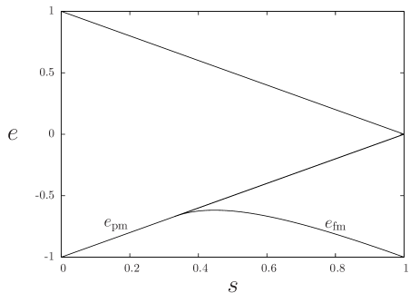
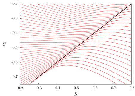
  Figure 13: Left panel: the two regimes in the $(s,e)$ plane for the $p=2$ model. Right panel: a zoom of the spectrum obtained by numerical diagonalization for $N=80$ around the line $e=-(1-s)$ where the gaps between excited ferromagnetic states are no longer exponentially small.

• for $p\geq 3$ odd, the spectrum is symmetric under $e\to-e$ (as explained at the end of Sec. III.1), we shall thus describe only its part with negative $e$. The equation (11) has only $m=0$ as a solution for $s\leq s_{\rm sp}$, with an associated energy $e_{\rm pm}(s)=-(1-s)$, while for $s\geq s_{\rm sp}$ there are three solutions $0<m_{\rm i}(s)<m_{*}(s)$ with energies $e_{\rm pm}(s)$, $e_{\rm i}(s)$ and $e_{\rm fm}(s)$. These three energy curves are drawn on the plots of Fig. 14 for $p=3$; the energies corresponding to doubly-degenerate eigenstates with exponentially small gaps between them are in the range $[\max[e_{\rm fm}(s),e_{\rm pm}(s)],e_{\rm i}(s)]$ for $s\geq s_{\rm sp}$. On the right panel we have superimposed the spectrum for $N=320$, one sees indeed that the avoided crossings occur precisely in this regime. All other authorized values of the energy correspond to non-degenerate eigenvalues.

        

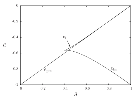
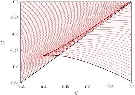
  Figure 14: Left: the three areas in the negative energy part of the spectrum of $p=3$. Right: a blow up of the data from numerical diagonalization in the region of exponentially small gaps for $N=320$.

• for $p\geq 4$ even, the phenomenology is mixed between the one of the $p=2$ and the $p\geq 3$ odd cases. Three zones are to be distinguished in the $(e,s)$ plane (see Fig. 15). One corresponds to the ferromagnetic phase, with doubly quasi-degenerate eigenstates of opposite magnetizations, for $s\geq s_{\rm c}$ and $e\in[e_{\rm gs}(s),e_{\rm pm}(s)]$. In the area $s\geq s_{\rm sp}$, $e\in[\max[e_{\rm fm}(s),e_{\rm pm}(s)],e_{\rm i}(s)]$ there are three valid solutions of Eq. (29). As explained at the end of Sec. III.7.2 avoided crossings in this area, that are of order $e^{-N\gamma(s,e)}$, only occur between continuation of levels coming from the paramagnetic zone and combination of ferromagnetic quasi-eigenvectors that have the same parity under the reversal of the longitudinal magnetization. The splitting between symmetric and antisymmetric combinations of ferromagnetic states is much smaller, of order $e^{-2N\gamma(s,e)}$. This phenomenon comes from the additional symmetry of even $p$ models discussed at the end of Sec. III.1, and is illustrated on the right panel of Fig. 15. The other authorized regime in the $(e,s)$ plane leads to single solutions of Eq. (29).

        

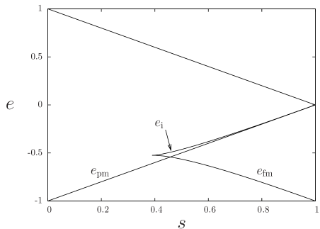
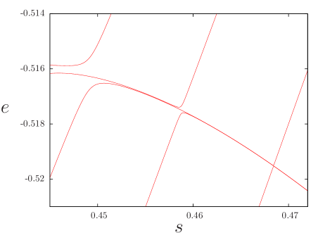
  Figure 15: Left: the three areas in the spectrum of the $p=4$ model. Right: avoided crossings between paramagnetic excited states and quasi-degenerate ferromagnetic excited states, for $p=4$ and $N=40$.

III.7.4 Exponentially small gaps encountered by the metastable states

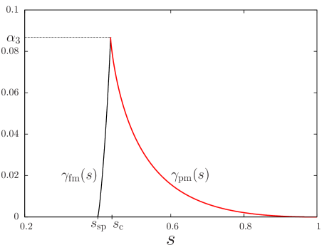
In view of the application of these computations to the annealing dynamics in Sec. IV, the most important case to consider is the size of the gaps encountered along the metastable continuations of the paramagnetic and ferromagnetic groundstates. We shall thus define $\gamma_{\rm pm}(s)=\gamma(s,e_{\rm pm}(s))$ for $s\in[s_{\rm c},1]$ and $\gamma_{\rm fm}(s)=\gamma(s,e_{\rm fm}(s))$ for $s\in[s_{\rm sp},s_{\rm c}]$. These quantities are plotted for $p=3$ in Fig. 16, along with an example of the functions $\varphi_{1,2}$ involved in the computation of $\gamma_{\rm pm}$ for one value of $s$. The numerical evaluation of these quantities is easy thanks to the explicit expression (69). One can also perform analytically some expansions around special values:

• $\gamma_{\rm fm}(s)$ vanishes at $s_{\rm sp}$ as $\widehat{\gamma}_{p}(s-s_{\rm sp})^{5/4}$, with the prefactor expressed as

  $$\widehat{\gamma}_{p}=\frac{6\sqrt{2}}{5}\frac{(p-1)^{\frac{5(p-3)}{8}}}{p^{\frac{5}{4}}(p-2)^{\frac{5p-12}{8}}}\left(1+p\frac{(p-2)^{\frac{p-2}{2}}}{(p-1)^{\frac{p-1}{2}}}\right)^{\frac{5}{2}}\ .$$ (71)

  The exponent $5/4$ is in agreement with the reasoning of botet83 recalled in Sec. III.7.2. Indeed the spinodal transition is in the universality class of cubic field theories, with the upper critical dimension (taking into account the imaginary time direction) $d_{\rm c}=5$, and the mean-field value of the critical exponent for the divergence of the correlation length $\nu_{\rm mf}=\frac{1}{4}$. One can also adapt the Finite Size Scaling argument of botet83 to predict that for large but finite values of $N$ the gaps encountered in the neighborhood of the spinodal should scale as $N^{-4/25}$. This follows from a scaling hypothesis of gaps of the form given in Eq. (68), combined with the exponent $x^{\prime}=4/5$ obtained above from the limit $s\to s_{\rm sp}^{+}$, and the closing of the finite gaps in the limit $s\to s_{\rm sp}^{-}$, argued to occur with an exponent 1/5 at the end of Sec. III.6.

• On the other hand the vanishing of $\gamma_{\rm pm}$ when $s\to 1$ is non-universal (i.e. depends on $p$), one finds indeed

  $$\gamma_{\rm pm}(s=1-\delta)\sim\widetilde{\gamma}_{p}\,\delta^{\frac{2}{p-2}}\ ,\qquad\widetilde{\gamma}_{p}=\frac{1}{2^{\frac{p}{p-2}}}\int_{0}^{1}{\rm d}x\,x\sqrt{1-x^{p-2}}\ .$$ (72)

• In the neighborhood of $s_{\rm c}$ the behavior of $\gamma_{\rm fm}$ and $\gamma_{\rm pm}$ exhibit a singularity of the form $(s-s_{\rm c})\ln(s-s_{\rm c})$, more precisely

  $$\gamma_{\rm pm}(s_{\rm c}+\delta)\sim\alpha_{p}+\widetilde{\eta}_{p}\,\delta\ln(\delta)\ ,\qquad\gamma_{\rm fm}(s_{\rm c}-\delta)\sim\alpha_{p}+\widehat{\eta}_{p}\,\delta\ln(\delta)\ ,$$ (73)

  where the constants $\widetilde{\eta}_{p}$ and $\widehat{\eta}_{p}$ are given by

  $$\widetilde{\eta}_{p}=\frac{(p-1)^{p-\frac{5}{2}}}{p^{\frac{p}{2}}(p-2)^{\frac{p-3}{2}}}\left(1+\frac{p^{\frac{p}{2}}(p-2)^{\frac{p-2}{2}}}{(p-1)^{p-1}}\right)^{2}\ ,\qquad\widehat{\eta}_{p}=\sqrt{(p-1)(p-2)}\,\widetilde{\eta}_{p}\ .$$ (74)

      

Figure 16: Left panel: the exponential rates $\gamma_{\rm pm}(s)$ and $\gamma_{\rm fm}(s)$ of the gaps encountered along the metastable continuation of the paramagnetic and ferromagnetic groundstates, for $p=3$. Right panel: the functions $\varphi_{1,2}$ yielding $\gamma_{\rm pm}(s=0.45)$.

IV Quantum annealing of the models

This section is devoted to the study of the annealing of the models whose static properties were considered above, and is organized as follows. We shall first (in Sec. IV.1) define precisely the dynamics and the quantities of interest to be studied in this context. Then we will review the phenomenology of the simple, two-level, Landau-Zener problem in Sec. IV.2 and discuss on this basis the expected features of the annealing dynamics. A further simplified model is introduced as an aside in Sec. IV.3, that will be used as a benchmark for the comparison with numerical results. The actual computations and results will then be presented in two sections, divided according to the scaling of the annealing time with the system size; in Sec. IV.4 we shall consider annealings on exponentially large times, while in Sec. IV.5 we will study the behavior of the dynamics when the thermodynamic limit is taken for a finite annealing rate. The main results of Sec. IV.4 and IV.5 are presented for odd values of $p\geq 3$ for which the phase-transition is first order and not mixed up with the quasi-degeneracy of the ferromagnetic states. We briefly comment in Sec. IV.6 on the behavior for even values of $p$, in particular $p=2$ (the Curie-Weiss model) whose annealing was already studied in santoro08 ; solinas08 ; itin09_1 ; itin09_2 .

IV.1 Definitions

As sketched in the introduction the quantum annealing procedure, or quantum adiabatic algorithm, aims at finding the groundstate of some final Hamiltonian $\widehat{H}_{\rm f}$ via an interpolation from an initial Hamiltonian $\widehat{H}_{\rm i}$ whose groundstate is easy to construct. The system evolves from time $t=0$ to $t=T$, the total running time of the algorithm, according to the Schrödinger equation with an Hamiltonian interpolating (for instance linearly) between $\widehat{H}_{\rm i}$ and $\widehat{H}_{\rm f}$. In terms of the reduced time $s=t/T\in[0,1]$, this reads

$$\frac{i}{T}\frac{{\rm d}}{{\rm d}s}|\phi_{T}(s)\rangle=\widehat{H}(s)|\phi_{T}(s)\rangle\ ,\qquad\widehat{H}(s)=(1-s)\widehat{H}_{\rm i}+s\widehat{H}_{\rm f}\ ,$$ (75)

with the initial condition that $|\phi_{T}(0)\rangle$ is the (normalized) groundstate of $\widehat{H}_{\rm i}$ (we set $\hbar=1$ from now on). The outcome of the algorithm for an annealing time $T$ is thus the final state $|\phi_{T}(1)\rangle$, which ideally, if $T$ is much larger than the adiabatic time, is close to the groundstate of $\widehat{H}_{\rm f}$.

It is however interesting, in particular for the approximability issues mentioned in the introduction, to study this procedure also for $T$ smaller than the adiabatic time. We shall quantify the deviation from adiabaticity by computing the final energy density defined as

$$e_{\textrm{fin}}(T,N)=\frac{1}{N}\langle\phi_{T}(1)|\widehat{H}_{\rm f}|\phi_{T}(1)\rangle\ ,$$ (76)

and comparing it to the groundstate energy density $e_{\rm gs}$ of the final Hamiltonian $\widehat{H}_{\rm f}$: the residual energy density is thus $e_{\textrm{res}}=e_{\textrm{fin}}-e_{\rm gs}$. Another relevant energy density to compare $e_{\textrm{fin}}$ to is the trivial one achieved when the interpolation time vanishes, i.e. when one computes the average energy of the final Hamiltonian with respect to the groundstate of the initial one: $e_{\textrm{triv}}=\frac{1}{N}\langle\phi_{T}(0)|\widehat{H}_{\rm f}|\phi_{T}(0)\rangle$. Indeed $e_{\textrm{gain}}=e_{\textrm{triv}}-e_{\textrm{fin}}$ is the gain in energy density that is achieved by the evolution during the time $T$. Note that with the normalization we chose for the models one has $e_{\rm gs}=-1$ and $e_{\textrm{triv}}=0$.

Our analytical results will all be obtained in the thermodynamic limit $N\to\infty$, but with two different scaling of $T$ with $N$ that shall be distinguished typographically. If $T$ is kept fixed when $N$ diverges we shall denote

$$e_{\textrm{fin}}(T)=\lim_{N\to\infty}e_{\textrm{fin}}(T,N)\ ;$$ (77)

this regime will be studied in Sec. IV.5. On the other hand if $T$ scales exponentially with $N$ (as in Sec. IV.4) we call $\tau$ this exponential rate and define

$$e_{\textrm{fin}}(\tau)=\lim_{N\to\infty}e_{\textrm{fin}}(T=e^{N\tau},N)\ .$$ (78)

We shall argue in the following that, as far as intensive quantities like the energy density are concerned, these two regimes are the only relevant ones for $p\geq 3$ (see Sec. IV.6 for a discussion of the different case $p=2$), i.e. polynomial scalings of $T$ with $N$ are just limiting cases of the two regimes above. Note also that in the thermodynamic limit, for both regimes, the quantum fluctuations of the final energy density are neglectible, hence a description in terms of the average energy only is meaningful.

The definitions above are valid for any choice of the inital and final Hamiltonians. From the point of view of potential applications they are of course most interesting when $\widehat{H}_{\rm f}$ has a groundstate that is a priori hard to find and when it is easy to prepare the system in the groundstate of $\widehat{H}_{\rm i}$. In the following we shall consider the dynamics of the annealing of the models whose statics were studied in the first part, that is use a $p$-spin interaction and a transverse field as initial and final Hamiltonian. Obviously neither of these Hamiltonians has a groundstate which is hard to find, hence they can only be considered as toy models for the application of the quantum adiabatic algorithm. However they share some properties (first-order transitions, metastability, spinodals) with more realistic random combinatorial optimization problems qXOR ; young10 , while being much easier to study both analytically and numerically. Because of this unrealistic character both choices of the transverse field as $\widehat{H}_{\rm i}$ and the ferromagnetic interaction as $\widehat{H}_{\rm f}$ or viceversa are equally relevant, and it will be very instructive to consider these two types of evolution. Let us define them more precisely:

• The annealing towards the ferromagnet corresponds to the choice $\widehat{H}_{\rm i}=-N\widehat{m}^{x}$, $\widehat{H}_{\rm f}=-N(\widehat{m}^{z})^{p}$, i.e. $\widehat{H}(s)=-(1-s)N\widehat{m}^{x}-sN(\widehat{m}^{z})^{p}$ is precisely the Hamiltonian (2) studied in the first part of the paper.

• The annealing towards the paramagnet corresponds to the reverse choice $\widehat{H}_{\rm i}=-N(\widehat{m}^{z})^{p}$, $\widehat{H}_{\rm f}=-N\widehat{m}^{x}$, in other words the evolution with the Hamiltonian (2) is made with $s$ decreasing from 1 to 0. To avoid confusion we shall denote $u=1-s$ instead of $s$ the reduced time in this case, i.e. study the following equation:

  $$\frac{i}{T}\frac{{\rm d}}{{\rm d}u}|\phi_{T}(u)\rangle=[-N(1-u)(\widehat{m}^{z})^{p}-Nu\,\widehat{m}^{x}]|\phi_{T}(u)\rangle\ .$$ (79)

Note that in all these cases the groundstate of the initial Hamiltonian $\widehat{H}_{\rm i}$ belongs to the fully symmetric sector of maximal spin. The instantaneous Hamiltonian $\widehat{H}(s)$ is block diagonal with respect to the spin decomposition for all values of $s$, in consequence the state $|\phi_{T}(s)\rangle$ remains in the maximal spin sector $K=0$ all along the evolution.

IV.2 Finite duration Landau-Zener problem and its expected consequences

The Landau-Zener problem landau32 ; zener32 is the simplest example of a quantum evolution with a time-evolving Hamiltonian. It involves two levels of linearly varying energy with a fixed coupling between them:

$$i\frac{{\rm d}}{{\rm d}t}\begin{pmatrix}\psi_{1}(t)\\ \psi_{2}(t)\end{pmatrix}=\begin{pmatrix}at&\epsilon\\ \epsilon&-at\end{pmatrix}\begin{pmatrix}\psi_{1}(t)\\ \psi_{2}(t)\end{pmatrix}\ .$$ (80)

The initial condition is given by $\psi_{1}(t\to-\infty)=1$, i.e. the system is initially in its groundstate. The probability of transition to the excited state after an infinite time can be computed exactly (see rojo10 ; wittig05 ; volkov06 for modern derivations) and yields $P_{\rm exc}=\underset{t\to+\infty}{\lim}|\psi_{1}(t)|^{2}=\exp(-\pi a\epsilon^{2})$. It is thus a function of the product between the square of the minimal gap $\epsilon$ at $t=0$ and the velocity $a$ of variation of the energies of the levels.

Variations of the Landau-Zener model that account for a finite duration of the interaction have been studied in great details in vitanov96 ; vitanov99 . Consider for instance an evolution with a reduced time $s\in[0,1]$ corresponding to a total physical time $T$, with two levels that have an avoided crossing at $s=1/2$:

$$i\frac{1}{T}\frac{{\rm d}}{{\rm d}s}\begin{pmatrix}\psi_{1}(s)\\ \psi_{2}(s)\end{pmatrix}=\begin{pmatrix}a(s-\frac{1}{2})&\epsilon\\ \epsilon&-a(s-\frac{1}{2})\end{pmatrix}\begin{pmatrix}\psi_{1}(s)\\ \psi_{2}(s)\end{pmatrix}\ .$$ (81)

The probability $P_{\rm exc}(a,\epsilon,T)$ that the evolution starting from the groundstate at $s=0$ leads to the excited state at $s=1$ can be expressed in terms of special functions vitanov96 and simplified in various asymptotic limits according to the relative ordering of $a,\epsilon$ and $1/T$. In the present context the relevant regime corresponds to $a$ fixed, $\epsilon\to 0$ and $T\to\infty$. Then $P_{\rm exc}$ has a scaling form if $T$ diverges as $\epsilon^{-2}$, more precisely

$$\lim_{\epsilon\to 0}P_{\rm exc}(a,\epsilon,T=\alpha\epsilon^{-2})=\exp[-\pi\alpha/a]\ .$$ (82)

If one further assumes that both $T$ and $\epsilon$ scales exponentially with a large parameter $N$, according to $\epsilon(N)=e^{-\gamma N}$ and $T=e^{\tau N}$, then the probability of excitation reduces to

$$\lim_{N\rightarrow\infty}P_{\rm exc}=\theta(2\gamma-\tau)\ ,$$ (83)

with $\theta(x)$ the Heaviside step function, i.e. on this scale either the evolution is sufficiently slow and the system follows adiabatically the groundstate or it is too fast and with probability 1 the system goes into the excited state.

Let us now explain the intuitive picture for the dynamics of the $p$-spin ferromagnetic model (with an odd value of $p\geq 3$) in the large $N$ limit, that arises from the combination of the study of this two-level problem and of the results of Sec. III (a similar reasoning can be found for instance in santoro02 ). Consider first the annealing towards the ferromagnet, for a large evolution time $T$, starting from the groundstate at $s=0$. As long as $s<s_{\rm c}$ the gap between the groundstate and the first excited state remains finite, hence for times sufficiently large (but independent of the system size), it is expected that the system will remain in the instantaneous ground state. There occurs at $s_{\rm c}$ an avoided crossing with an exponentially small gap of order $e^{-N\alpha_{p}}$. Transposing the results of the two-level problem, two cases have to be distinguished. If the evolution time is exponentially large, $T=e^{\tau N}$, and if $\tau\geq 2\alpha_{p}$, then the system follows adiabatically the groundstate at the avoided crossing, and continues on the instantaneous groundstate. Otherwise the system is in the first excited state just after the crossing, i.e. on the metastable continuation of the paramagnetic groundstate. We have seen that this state encounters a series of avoided crossings, that lead to gaps of order $e^{-N\gamma_{\rm pm}(s)}$. Let us assume that all these avoided crossings are independent, and can be treated as in a two-level problem. Then, if the evolution time is $T=e^{N\tau}$, one is led to the conclusion that the system will remain in the metastable groundstate until the value $s_{\rm turn}$ such that $\tau=2\gamma_{\rm pm}(s_{\rm turn})$, and from thereon follows the excited ferromagnetic state that crossed the paramagnetic metastable state in $s_{\rm turn}$. As there is no spinodal limit for the metastable paramagnet $\gamma_{\rm pm}(s)>0$ for all $s<1$. Hence for an evolution on sub-exponential times $T$ the system should follow the paramagnet until $s=1$, which leads to a vanishing energy density gain with respect to the trivial one.

A similar reasoning in the case of the annealing towards the paramagnet reveals a richer phenomenology. For an exponentially large annealing time $e^{N\tau}$ with $\tau>2\alpha_{p}$ the groundstate is followed during the whole evolution. If $\tau<2\alpha_{p}$ the metastable ferromagnetic state will be followed until the turning point $u_{\rm turn}$ where $\tau=2\gamma_{\rm fm}(1-u_{\rm turn})$, then the system follows the paramagnetic excited state that rejoins the metastable ferromagnet at the turning point. There is however an important difference with respect to the reverse direction of annealing: here the ferromagnet has a spinodal limit of metastability. Hence an evolution on an exponentially long time $e^{N\tau}$, but for arbitrarily small values of $\tau$, yields a non-trivial (negative) energy density. In addition the regime of large but sub-exponential $T$ can be expected to be much richer than in the previous case: the ferromagnet will be followed for $u<u_{\rm sp}=1-s_{\rm sp}$, but for subsequent times this analysis in terms of level crossings can give no clue.

In this reasoning we have assumed that the various level crossings can be treated independently one from the others, and apply to each of them the results of a simple two-level problem. Arguments in favor of this assumption can be found from static schulman76 and dynamical vitanov99 ; volkov06 considerations: as can be seen on the drawings of the spectrum (see for instance the right panel of Fig. 6), an avoided crossing with an exponentially small gap affects notably the two colliding levels on an interval of $s$ which is also exponentially small. On the other hand two successive crossings are located at values of $s$ which are distant of order $1/N$. Similarly in the dynamical case the “duration” of a crossing (as defined in vitanov99 ) should go like $\exp((-\gamma+\tau)N)$, and therefore the influence of a crossing should spread on a range of $s$ of order at most $\exp(-\gamma N)$.

In the following sections we shall present the explicit results obtained from this reasoning, and compare them with the results of numerical integration of Schrödinger’s equation for finite values of $N$. In particular we will test the assumption of independence of the different crossings. The numerical results for the annealing of the $p$-spin model having strong finite-size corrections, we shall first introduce a simplified model that shares some of the properties of the $p$-spin model but with smaller finite-size effects.

IV.3 A further simplified model (the $p\to\infty$ limit)

We shall introduce here a simplified version of the models under study, first defining it formally and discussing afterwards its relationship with the main models of the article and with previous works.

We consider an interpolating Hamiltonian $\widehat{H}_{\bullet}(s)$ acting on the fully symmetric subspace of dimension $N+1$. It is given by $\widehat{H}_{\bullet}(s)=(1-s)\widehat{J}-Ns\widehat{m}^{x}$, with the initial Hamiltonian $\widehat{H}_{\rm i}=\widehat{J}$ defined by its matrix elements in the $x$-diagonal basis,

$$\phantom{}{}_{x}\langle m;0|\widehat{J}|m^{\prime};0\rangle_{x}=-ND_{m}D_{m^{\prime}}\ ,\qquad D_{m}=\sqrt{\frac{1}{2^{N}}\binom{N}{N\frac{1+m}{2}}}\ .$$ (84)

It is thus a matrix of rank 1, with a single eigenvalue equal to $-N$ and all other eigenvalues equal to $0$. The spectrum of $\widehat{H}_{\bullet}(s)$ is presented on the left panel of Fig. 17. As $\widehat{J}$ is of rank one the spectrum of $\widehat{H}_{\bullet}(s)$ is essentially equal to the one of $-Ns\widehat{m}^{x}$ (see for instance lowrank for general results on low rank perturbation theory). There is however a major difference: the isolated eigenvalue of energy density $e=-(1-s)$ is continued as a metastable state for $s\in[1/2,1]$, with exponentially small avoided crossings of order $e^{-N\gamma_{\bullet}(s)}$. The computation of $\gamma_{\bullet}(s)$ is presented in Appendix B.1, and yields the explicit formula

$$\gamma_{\bullet}(s)=-\frac{1}{2}\ln s+\frac{2s-1}{4s}\ln(2s-1)\ ;$$ (85)

this function is plotted on the right panel of Fig. 17. For the reasons explained above one expects that the annealing of the model on sub-exponential time scales yields a vanishing final energy density, as the metastable continuation of the groundstate exists until $s=1$; this is confirmed by the analysis presented in Appendix  B.2. Exponentially slow annealings with $0<\tau<\ln 2$ (i.e. $T\ll 2^{N}$) should however reach a non-trivial negative energy density, larger than the one of the groundstate but smaller than the trivial one, $e_{\rm gs}<e_{\textrm{fin}}(\tau)<e_{\textrm{triv}}$ in the notations of Sec. IV.1.

Figure 17: Left: spectrum of the operator $\widehat{H}_{\bullet}(s)$ as a function of $s$, for $N=80$. In the thermodynamic limit the metastable continuation of the groundstate at $s\leq 1/2$ exists until $s=1$. Right: The exponential rate of closing of the gaps at the avoided crossings $\gamma_{\bullet}(s)$, defined in Eq. (85).

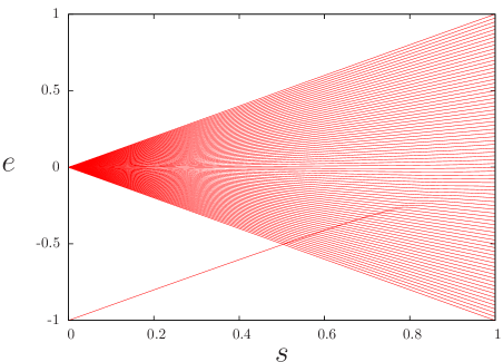
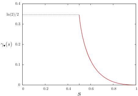
This simplified model is actually (almost) the $p\to\infty$ limit (with $p$ odd, and the limit on $p$ taken before the limit on $N$) of the models studied in the main part of this paper (and was discussed in these terms in jorg10 ): in the $z$-basis $\widehat{J}$ is diagonal, with matrix elements $\phantom{}{}_{z}\langle m;0|\widehat{J}|m;0\rangle_{z}=-N\delta_{m,1}$, to be compared with $\underset{p\to\infty}{\lim}\phantom{}_{z}\langle m;0|-N(\widehat{m}^{z})^{p}|m;0\rangle_{z}=-N\delta_{m,1}+N\delta_{m,-1}$ if the limit is taken with $p$ odd. If one focuses on the low-energy part of the spectrum, one can view the evolution of the simplied model as the evolution towards the paramagnet of the $p$-spin model in the large odd $p$ limit.

Another justification for the introduction of this simplified model can be given as follows. Assume that one is given an arbitrary Hamiltonian $\widehat{H}_{\rm f}$, diagonal in the computational basis of the $2^{N}$ classical configurations of spins, as an optimization problem, and that the problem is to be solved without using any information about the local structure of these energies in the configuration space. Then the most natural starting Hamiltonian $\widehat{H}_{\rm i}$ for an interpolation is the one connecting any two configurations of the Hilbert space with equal probability,

$$\widehat{H}_{\rm i}=\widehat{J}=-\frac{N}{2^{N}}\sum_{\underline{\sigma},\underline{\sigma}^{\prime}}|\underline{\sigma}\rangle\langle\underline{\sigma}^{\prime}|=-N|X\rangle\langle X|\ ,\quad\text{with}\ \ |X\rangle=\frac{1}{2^{N/2}}\sum_{\underline{\sigma}}|\underline{\sigma}\rangle\ ,$$ (86)

where the normalization chosen is such that $\widehat{J}$ has one eigenvector $|X\rangle$ with eigenvalue $-N$ and $2^{N}-1$ eigenvectors with eigenvalue $0$. Let us denote $\{E_{\alpha}\}_{\alpha\in[1,M]}$ the distinct energies of $\widehat{H}_{\rm f}$, $d_{\alpha}$ the number of configurations $\underline{\sigma}$ on which $\widehat{H}_{\rm f}$ takes the value $E_{\alpha}$, and $\widetilde{\mathcal{H}}$ the $M$-dimensional Hilbert space generated by the symmetric combinations of the states of a given energy:

$$\widetilde{\mathcal{H}}=\textrm{span}\left\{|\alpha\rangle\right\}\ ,\qquad|\alpha\rangle=\frac{1}{\sqrt{d_{\alpha}}}\sum_{\underline{\sigma},H_{\rm f}(\underline{\sigma})=E_{\alpha}}|\underline{\sigma}\rangle\ .$$ (87)

Then the ground state $|X\rangle$ of $\widehat{J}$ is in $\widetilde{\mathcal{H}}$, and so is, for any $s$, the vector $|\phi_{T}(s)\rangle$ obtained by the evolution according to the Schrödinger equation with $\widehat{H}(s)=(1-s)\widehat{J}+s\widehat{H}_{\rm f}$ as interpolating Hamiltonian. The dynamics can thus be studied in the symmetric subspace $\widetilde{\mathcal{H}}$, in which the matrix elements of $\widehat{H}(s)$ are given by

$$\langle\alpha|\widehat{H}(s)|\beta\rangle=s\delta_{\alpha,\beta}E_{\alpha}-(1-s)N\frac{\sqrt{d_{\alpha}d_{\beta}}}{2^{N}}\ .$$ (88)

The simplified model defined at the beginning of this section is thus a representative example of this more general construction, in which we chose $M=N+1$, with equally spaced levels $E_{\alpha}$ between $-N$ and $+N$, each with a binomial degeneracy. The quantum annealing with such an unstructured Hamiltonian $\widehat{J}$ has been studied in farhi08 . In the context of Grover Grover search problem (i.e. with a golf course potential $\widehat{H}_{\rm f}$ having a single low energy level), it was shown in roland01 that a modification of the annealing procedure could reproduce Grover’s quadratic speedup. By slowing down the interpolation in the neighborhood of the avoided crossing one can indeed reduce the adiabatic time to $O(2^{N/2})$.

IV.4 Annealing on exponentially large times

IV.4.1 The simplified model

Let us compute the final energy $e_{\textrm{fin}}(\tau)$ after an exponentially long annealing of duration $T=e^{N\tau}$, for the simplified model of Sec. IV.3, following the reasoning of Sec. IV.2. The turning point $s_{\rm turn}$ up to which the metastable state is followed is given implicitly by $2\gamma_{\bullet}(s_{\rm turn}(\tau))=\tau$, where the expression of $\gamma_{\bullet}$ is given in Eq. (85) (if $\tau>2\gamma_{\bullet}(1/2)=\ln 2$ we set $s_{\rm turn}(\tau)=1/2$). The final energy at the end of the annealing is then given by the continuation of the state that crosses the metastable state at $s_{\rm turn}$. For this simple model where energy levels are at leading order linear functions of $s$ except at the crossings, this yields:

$$e_{\textrm{fin}}(\tau)=-\frac{1-s_{\rm turn}(\tau)}{s_{\rm turn}(\tau)}=1-\frac{1}{\gamma_{\bullet}^{-1}(\tau/2)}\ ,$$ (89)

where $\gamma_{\bullet}^{-1}$ is the functional inverse of $\gamma_{\bullet}$, with the convention that $\gamma_{\bullet}^{-1}(z)=1/2$ if $z>\frac{\ln 2}{2}$.

A comparison of this analytical prediction with the results obtained by numerical integration of the Schrödinger equation (see Appendix C for details on the procedure we used) is presented in Fig. 18. The left panel displays the result of Eq. (89) along with curves $e_{\textrm{fin}}(T=e^{N\tau},N)$ obtained numerically for some finite values of $N$. We extrapolated these results in the $N\to\infty$ limit with finite size corrections of the form $e_{\textrm{fin}}(T=e^{N\tau},N)=a(\tau)+b(\tau)\frac{\ln N}{N}+c(\tau)\frac{1}{N}+o(1/N)$, a form that can be expected to arise because of polynomial corrections to the exponentially small gaps; the inset shows the very good quality of such a fit already for small values of $N$. The extrapolated curve $a(\tau)$ agrees with the analytical prediction (89) within $1\%$.

The right panel of Fig. 18 provides a further confirmation of the analysis in terms of independent two level Landau-Zener problems. The black symbols with error bars represent the quantum average and standard deviation of the instantaneous energy,

$$e_{T}(s)=\frac{1}{N}\langle\phi_{T}(s)|\widehat{H}(s)|\phi_{T}(s)\rangle\ ,\qquad\sigma_{T}(s)=\frac{1}{N}\sqrt{\langle\phi_{T}(s)|\widehat{H}(s)^{2}|\phi_{T}(s)\rangle-\left(\langle\phi_{T}(s)|\widehat{H}(s)|\phi_{T}(s)\rangle\right)^{2}}\ ,$$ (90)

computed numerically during an evolution with $N=64$, $T=e^{N\tau}$ for $\tau=0.2$. One observes indeed that the average instantaneous energy follows the metastable groundstate across several crossings, until the turning point after which it follows adiabatically the levels crossed there. The standard deviation is almost constant in time except around the turning point where it grows slightly, reflecting the fact that for finite $N$ a few levels (those with gaps close to $T^{-1/2}$) get populated. The independence of the crossings is even more apparent in the inset, which shows that the slope of $e_{T}(s)$ jumps significantly for three values of $s$ that correspond precisely to the locations of avoided crossings.

Figure 18: Left panel: final energy density for the evolution of the simplified model as a function of $\tau=(\log T)/N$. The solid line is the analytic prediction (89). The symbols are the results of the integration of Schrödinger equation for $N=16,36,64,128$, and an extrapolation to $N\to\infty$ using corrections in $(\ln N)/N$ and $1/N$. The insets shows this fit for $\tau=0.1$, with a fitting function of the form $f(N)=a+b\ln(N)/N+c/N$, with the results of a best fit on $N\geq 20$ given by $a=-0.438$, $b=-1.463$, $c=2.926$. Right panel: black symbols and error bars represent the average and standard deviation of the instantaneous energy, for the evolution of the simplified model with $N=64$, $\tau=0.2$. The red lines correspond to the spectrum of $\widehat{H}_{\bullet}(s)$. The inset is a zoom around the turning point, the arrow on the right is the prediction of Eq. (89) for the final energy density in the thermodynamic limit.

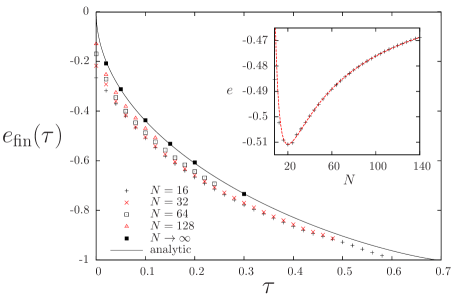
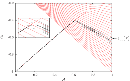
For completeness let us state the asymptotic expansions of $e_{\textrm{fin}}(\tau)$ around $\tau=0$ and $\tau=\ln 2$, that are easily deduced from the behavior of $\gamma_{\bullet}(s)$ in $s=1$ and $s=1/2$, respectively, and read

$$e_{\textrm{fin}}(\tau)\underset{\tau\to 0}{\sim}-\sqrt{2\tau}\ ,\qquad e_{\textrm{fin}}(\tau=\ln 2-\delta)\underset{\delta\to 0^{+}}{\sim}-1+2\frac{\delta}{\ln(1/\delta)}\ .$$ (91)

IV.4.2 The annealing towards the ferromagnet

We now follow the same reasoning for the annealing of the $p$-spin model towards the ferromagnet. The turning point $s_{\rm turn}$ is given by $s_{\rm turn}(\tau)=\gamma_{\rm pm}^{-1}(\tau/2)$, where the function $\gamma_{\rm pm}$ was computed in Sec. III.7.4 and plotted on the left panel of Fig. 16. We adopt again the convention that $\gamma_{\rm pm}^{-1}(z)=s_{\rm c}$ if $z\geq 2\alpha_{p}$. As already mentioned in Sec. III.5 the computation of $e_{\textrm{fin}}(\tau)$ is then completed by an iso-density argument: for $s\geq s_{\rm turn}(\tau)$ we assume that the evolution follows adiabatically the eigenstate that made an avoided crossing with the paramagnetic metastable state at $s_{\rm turn}$. Because of the absence of any level crossing in this regime the number of eigenvalues below the one whose energy we want to follow is constant, by definition. Hence $e_{\textrm{fin}}$ is fixed by the condition

$${\cal D}_{0}(s_{\rm turn}(\tau),-(1-s_{\rm turn}(\tau)))={\cal D}_{0}(1,e_{\textrm{fin}}(\tau))=\frac{1-(-e_{\textrm{fin}}(\tau))^{1/p}}{2}\ ,$$ (92)

where the integrated density of states ${\cal D}_{0}(s,e)$ is given in Eq. (45), and the last equality follows from its explicit expression when $s=1$, $p$ is odd and $e\leq 0$. This prediction is displayed in the left panel of Fig. 19, along with results of the numerical integration of the Schrödinger equation for finite $N$. The finite-size effects in these results are much larger than for the simplified model. The extrapolation towards $N\to\infty$ was done searching the value of $\tau$ that corresponds to a given final energy density instead of the contrary (see the caption of Fig. 19 for details), and gives a satisfactory agreement with the analytic prediction.

Figure 19: The final energy density for the evolution on exponentially large times, as a function of $\tau=(\log T)/N$. The left (resp. right) panel corresponds to the annealing towards the ferromagnet (resp. paramagnet) for $p=3$. The solid lines at the bottom are the analytic prediction from Eq. (92) for the left panel, and Eq. (96) for the right one. The other lines with symbols results from the integration of Schrödinger equation for various finite sizes. The black symbols on top of the analytic predictions are the extrapolation in the $N\to\infty$ limit of the numerical results. The latter was performed by fitting, for various values of $e$, the (exponential) time $\tau(N)$ such that $e_{\textrm{fin}}(T=e^{N\tau(N)},N)$ crossed $e$, with a fitting function of the form $\tau(N)=\tau+\text{cst}\frac{\ln N}{N}+\text{cst}\frac{1}{N}$. We show in the insets the details of the fit for $e=-0.5$ (left panel) and $e=-0.945$ (right panel).

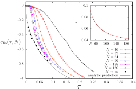
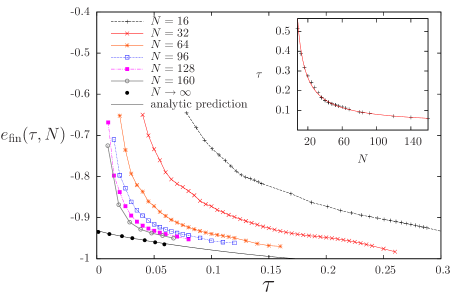
The final energy density vanishes in the $\tau\to 0$ limit, as the paramagnetic metastable state has no spinodal and can thus be continued until $s=1$. A more precise asymptotic statement can be obtained by studying the behavior of the integrated density of states close to $s=1$, namely

$${\cal D}_{0}(1-\delta,-\delta)\sim\frac{1}{2}-d_{p}\,\delta^{\frac{1}{p}}\ ,\qquad d_{p}=2^{\frac{1-p}{p}}-\frac{1}{2\pi}\int_{0}^{2}{\rm d}x\,x^{\frac{1-p}{p}}\text{acos}\,(1-x)\ ,$$ (93)

for odd values of $p$. Combining this expansion with the one of $\gamma_{\rm pm}(s=1-\delta)$ stated in Eq. (72) yields

$$e_{\textrm{fin}}(\tau)\underset{\tau\to 0}{\sim}-e_{p}\,\tau^{\frac{p-2}{2}}\ ,\qquad e_{p}=2^{\frac{p+2}{2}}d_{p}^{p}\,\widetilde{\gamma}_{p}^{\frac{2-p}{2}}\ .$$ (94)

On the other hand the behavior of $e_{\textrm{fin}}(\tau)$ for (exponential) times slightly smaller than the adiabatic time $\tau=2\alpha_{p}$ corresponds to the limit where $s_{\rm turn}\to s_{\rm c}^{+}$. One can thus invert the expansion (73) for the behavior of $\gamma_{\rm pm}$ around $s_{\rm c}$ to obtain the behavior of $s_{\rm turn}(\tau\to 2\alpha_{p})$. Noting that ${\cal D}_{0}(s,-(1-s))$ has a finite derivative with respect to $s$ in $s_{\rm c}$, one obtains finally after the simplification of various constants:

$$e_{\textrm{fin}}(\tau=2\alpha_{p}-\delta)\underset{\delta\to 0^{+}}{\sim}-1+2p\frac{\delta}{\ln(1/\delta)}\ ,$$ (95)

whose form is similar to the one found for the simplified model in Eq. (91).

IV.4.3 The annealing towards the paramagnet

The annealing towards the paramagnet can be treated along the same lines. We recall that in this case the interpolation parameter is $u=1-s$. The evolution follows the metastable ferromagnet until the turning point $u_{\rm turn}\in[1-s_{\rm c},1-s_{\rm sp}]$ such that $\tau=2\gamma_{\rm fm}(1-u_{\rm turn})$, with $\gamma_{\rm fm}(s)$ the function computed in Sec. III.7.4 and plotted on the left panel of Fig. 16. The isodensity argument for the continuation of the evolution in the regime $u\geq u_{\rm turn}$ reads then

$${\cal D}_{0}(1-u_{\rm turn}(\tau),e_{\rm fm}(1-u_{\rm turn}(\tau)))={\cal D}_{0}(0,e_{\textrm{fin}}(\tau))=\frac{1+e_{\textrm{fin}}(\tau)}{2}\ ,$$ (96)

the last equality being the consequence of the equidistance of the paramagnetic levels when $u=1$. A comparison of this analytical prediction with numerical results is shown on the right panel of Fig. 19. The agreement of the large $N$ extrapolation with the prediction of Eq. (96) is again satisfactory.

The small $\tau$ limit of this regime yields a non-trivial energy density, because the ferromagnetic metastable state has a spinodal limit of existence. It is given by the continuation of the paramagnetic state that goes to the spinodal point, and from the formula above reads:

$$\hat{e}_{\textrm{fin}}=\lim_{\tau\to 0}e_{\textrm{fin}}(\tau)=-1+2{\cal D}_{0}(s_{\rm sp},e_{\rm sp})\ .$$ (97)

We report the value of these energy densities for some values of $p$ in Table 2. For large $p$, using the asymptotics of (13), and the fact that the energy of paramagnetic levels become linear functions of $s$ in this limit, one gets the asymptotic behaviour $\hat{e}_{\textrm{fin}}\underset{p\to\infty}{\sim}-\frac{2}{\sqrt{p}}$, a form that agrees very well with the data in Table 2.

The correction of next order in $\tau$ is obtained from the asymptotic expansion of $\gamma_{\rm fm}$ around $s_{\rm sp}$, given in Eq. (71), which converts into $u_{\rm turn}(\tau)\sim 1-s_{\rm sp}-(\tau/2\widehat{\gamma}_{p})^{4/5}$. Let us define the positive constant

$$M_{p}=-\left.\frac{{\rm d}}{{\rm d}s}{\cal D}_{0}(s,e_{\rm fm}(s))\right|_{s=s_{\rm sp}^{+}}=\frac{1}{2\pi(1-s_{\rm sp})}\int_{m^{\prime}_{\rm sp}}^{m_{\rm sp}}{\rm d}m\,\frac{m_{\rm sp}^{p}-m^{p}}{\sqrt{(1-s_{\rm sp})^{2}(1-m^{2})-(e_{\rm sp}+s_{\rm sp}\,m^{p})^{2}}}\ ,$$ (98)

where $m^{\prime}_{\rm sp}$ is defined as the negative value of $m$ where the square root vanishes (one can notice that $M_{p}=\mathcal{G}(0)$, where $\mathcal{G}(z)$ is the scaling function defined in Eq. (57)). Then expanding in Eq. (96) one obtains the final energy density behaviour as

$$e_{\textrm{fin}}(\tau)\underset{\tau\to 0}{\sim}\hat{e}_{\textrm{fin}}-2M_{p}\left(\frac{\tau}{2\widehat{\gamma}_{p}}\right)^{\frac{4}{5}}\ .$$ (99)

The opposite limit of quasi-adiabatic times yields exactly the same formula for the energy density as in the simplified model (which is indeed its $p\to\infty$ limit), i.e.

$$e_{\textrm{fin}}(\tau=2\alpha_{p}-\delta)\underset{\delta\to 0^{+}}{\sim}-1+2\frac{\delta}{\ln(1/\delta)}\ .$$ (100)

$p$	$\Gamma_{\rm sp}$	$s_{\rm sp}$	$m_{\rm sp}$	$\hat{e}_{\textrm{fin}}$
3	1.5	0.6	0.7071	-0.9302
4	1.540	0.6062	0.8165	-0.8259
5	1.624	0.6189	0.8660	-0.7861
7	1.812	0.6443	0.9129	-0.6881
9	1.994	0.6660	0.9354	-0.6187
13	2.325	0.6993	0.9574	-0.5256
21	2.884	0.7426	0.9747	-0.4211
31	3.462	0.7759	0.9831	-0.3500

Table 2: Final energy for an annealing of the $p$-spin model towards the paramagnet, in the limit of “small exponential” times. The thermodynamic parameters of the system at the spinodal point are given by (13).

IV.5 Annealing on constant times

We now turn to a study of the dynamical properties of the previous models on time scales not growing exponentially fast with the size of the system. From the analysis of Sec. IV.2 we expect that for the simplified model and for the annealing towards the ferromagnet the final energy density vanishes on such time scales, because the metastable branch with exponentially small avoided crossing exists until $s=1$. This is confirmed for the simplified model by a technical analysis that is deferred to Appendix B.2. The annealing towards the ferromagnet can be treated via a semi-classical dynamical analysis itin09_1 ; itin09_2 ; sciolla11 , and this will confirm its triviality on constant time-scales. The same semi-classical analysis will on the other hand reveal a rich structure for the annealing towards the paramagnet on finite time scales.

IV.5.1 Semi-classical dynamics for the annealing towards the ferromagnet

Let us decompose the vector $|\phi_{T}(s)\rangle$ on the $z$-diagonal basis as

$$|\phi_{T}(s)\rangle=\underset{m\in{{\cal M}^{N}_{0}}}{\sum}\phi_{T}(m,s)|m;0\rangle_{z}\ .$$ (101)

The Schrödinger equation (75) is equivalent to a set of coupled equations for these coefficients,

$$\frac{i}{NT}\frac{\partial\phi_{T}(m,s)}{\partial s}=-s\,m^{p}\,\phi_{T}(m,s) - \frac{(1-s)}{2}\sqrt{1-m^{2}+\frac{2}{N}(1-m)}\ \phi_{T}\left(m+\frac{2}{N},s\right)$$ (102)

$$- \frac{(1-s)}{2}\sqrt{1-m^{2}+\frac{2}{N}(1+m)}\ \phi_{T}\left(m-\frac{2}{N},s\right)\ ,$$

which is the analog of (27) in the stationary case. The semi-classical dynamic Ansatz is $\phi_{T}(m,s)=e^{-N\varphi_{T}(m,s)}$, which yields in the large $N$ limit, with $T$ fixed, the evolution equation

$$-\frac{i}{T}\frac{\partial\varphi_{T}(m,s)}{\partial s}=-s\,m^{p}-(1-s)\sqrt{1-m^{2}}\cosh\left(2\varphi_{T}^{\prime}(m,s)\right)\ ,$$ (103)

where the prime denotes the derivation with respect to $m$. This corresponds to (28) with the replacement $e\to-\frac{i}{T}\frac{\partial\varphi_{T}}{\partial s}$. The initial condition is the groundstate of the pure transverse field, it is thus given by $\varphi_{T}(m,0)=\varphi_{0}(m)$, with $\varphi_{0}$ defined in Eq. (34). This partial differential equation is rather difficult to solve numerically. One can however make a further analytical simplification.

The computation of physical observables that are diagonal in the $\widehat{m}^{z}$ basis only requires the knowledge of the location of the minimum of the real part of the large deviation function $\varphi_{T}$, that we shall denote $q_{T}(s)=\arg\min_{m}\Re\varphi_{T}(m,s)$. In particular at the end of the evolution the final energy is given by $e_{\textrm{fin}}(T)=-q_{T}(1)^{p}$. It turns out, as explained in sciolla11 , that it is possible to write a closed system of two differential equations on $q_{T}(s)$ and its conjugate momentum, $\widetilde{q}_{T}(s)=-\partial_{m}\Im\varphi_{T}(q_{T}(s),s)$. The evolution equation (103) implies indeed

$$\begin{split}\frac{1}{T}\frac{{\rm d}}{{\rm d}s}q_{T}(s)&=\frac{\partial}{\partial\widetilde{q}}\mathcal{H}(q_{T}(s),\widetilde{q}_{T}(s),s)=2(1-s)\sqrt{1-q_{T}(s)^{2}}\sin(2\widetilde{q}_{T}(s))\ ,\\ \frac{1}{T}\frac{{\rm d}}{{\rm d}s}\widetilde{q}_{T}(s)&=-\frac{\partial}{\partial q}\mathcal{H}(q_{T}(s),\widetilde{q}_{T}(s),s)=s\,p\,q_{T}(s)^{p-1}-(1-s)\frac{q_{T}(s)}{\sqrt{1-q_{T}(s)^{2}}}\cos(2\widetilde{q}_{T}(s))\ .\end{split}$$ (104)

These are Hamilton equations of classical mechanics, with an Hamiltonian

$$\mathcal{H}(q,\widetilde{q},s)=-s\,q^{p}-(1-s)\sqrt{1-q^{2}}\cos(2\widetilde{q})$$ (105)

obtained from the differential operator on the r.h.s. of (103) by the canonical substitution $m\rightarrow q,i\frac{\partial\varphi_{T}}{\partial m}\rightarrow\widetilde{q}$. For the sake of completness we explain in Appendix D the derivation of (104) from (103), along the same lines as in sciolla11 ; note also that similar semi-classical equations can be obtained for fermionic models within the time-dependent Gutzwiller approximation ScFa10 .

One can in addition show that the average instantaneous energy of the evolution according to the Schrödinger equation is precisely equal to the classical Hamiltonian, namely

$$\lim_{N\to\infty}\frac{1}{N}\langle\phi_{T}(s)|\widehat{H}(s)|\phi_{T}(s)\rangle=\mathcal{H}(q_{T}(s),\widetilde{q}_{T}(s),s)\ .$$ (106)

Let us now conclude on the validity of the analysis of Sec. IV.2, i.e. that for annealing times $T$ that are constant in the thermodynamic limit the final energy $e_{\textrm{fin}}(T)$ vanishes. The initial condition $\varphi_{T}(m,s=0)=\varphi_{0}(m)$ implies $q_{T}(s=0)=\widetilde{q}_{T}(s=0)=0$. The point $(q,\widetilde{q})=(0,0)$ is a stationary point of $\mathcal{H}$ for all values of $s$, hence for all (finite when $N\to\infty$) values of the annealing time $T$ the solution of (104) is $q_{T}(s)=\widetilde{q}_{T}(s)=0$. In particular when $s=1$ the final energy is $e_{\textrm{fin}}(T)=-q_{T}(1)^{p}=0$.

IV.5.2 Semi-classical dynamics for the annealing towards the paramagnet

The semi-classical analysis of the annealing towards the paramagnet is more conveniently performed in the $x$-diagonal basis. We write $|\phi_{T}(u)\rangle=\underset{m\in{{\cal M}^{N}_{0}}}{\sum}\phi_{T}(m,u)|m;0\rangle_{x}$ with $\phi_{T}(m,u)=e^{-N\varphi_{T}(m,u)}$, and obtain from the Schrödinger equation (79) that $\varphi_{T}$ evolves according to

$$-\frac{i}{T}\frac{\partial\varphi_{T}(m,u)}{\partial u}=-u\,m-(1-u)(1-m^{2})^{p/2}\left(\cosh(2\varphi^{\prime}_{T}(m,u))\right)^{p}\ ,$$ (107)

the dynamical analog of Eq. (41). The initial condition corresponds to the groundstate of the $-(\widehat{m}^{z})^{p}$ term, and is thus given in this basis by $\varphi_{T}(m,u=0)=\varphi_{0}(m)$. The reduction of the partial differential equation (107) to an Hamiltonian system on $\{q_{T}(u),\widetilde{q}_{T}(u)\}$ follows the same lines as in the annealing towards the ferromagnet, and yields (see Appendix D for the derivation):

$$\begin{split}\frac{1}{T}\frac{{\rm d}}{{\rm d}u}q_{T}(u)&=\frac{\partial}{\partial\widetilde{q}}\mathcal{H}(q_{T}(u),\widetilde{q}_{T}(u),u)=2p(1-u)\left(1-q_{T}(u)^{2}\right)^{p/2}\sin(2\widetilde{q}_{T}(u))\left(\cos(2\widetilde{q}_{T}(u))\right)^{p-1}\ ,\\ \frac{1}{T}\frac{{\rm d}}{{\rm d}u}\widetilde{q}_{T}(u)&=-\frac{\partial}{\partial q}\mathcal{H}(q_{T}(u),\widetilde{q}_{T}(u),u)=u-p(1-u)q_{T}(u)\left(1-q_{T}(u)^{2}\right)^{p/2-1}\left(\cos 2\widetilde{q}_{T}(u)\right)^{p}\ .\end{split}$$ (108)

where the classical Hamiltonian is

$$\mathcal{H}(q,\widetilde{q},u)=-u\,q-(1-u)(1-q^{2})^{p/2}\cos(2\widetilde{q})^{p}\ .$$ (109)

The initial condition is $q_{T}(0)=\widetilde{q}_{T}(0)=0$, and the final energy is computed at the end of the evolution as $e_{\textrm{fin}}(T)=-q_{T}(1)$.

It is easy to integrate numerically the two coupled ordinary differential equations (108), and we present on Fig. 20 some results obtained in this way. The plot on the left panel shows the instantaneous energy density $\mathcal{H}(q_{T}(u),\widetilde{q}_{T}(u),u)$ as a function of the interpolation parameter $u$, for several (rather small) values of the annealing time $T$; the agreement with the integration of Schrödinger equation with $N=80$ is already excellent. On the right panel we concentrate on the final energy density, computed from the value of the solution of Hamilton equations in $u=1$, as a function of $T$. The finite size effects on the results of Schrödinger equation get stronger for larger values of $T$, yet their extrapolation with a correction term of order $1/N$ is in very good agreement with the classical dynamics prediction.

Figure 20: Annealing towards the paramagnet of the $p=3$ model, in the regime of constant times. Left: evolution of the instantaneous energy as a function of $u$, in the $N\to\infty$ limit with various values of $T$ (independent of $N$). The lines are the results of the integration of Hamilton equations of motion. The symbols are obtained via the integration of Schrödinger equation with $N=80$, for the $T$ values on which they fall on. The $T\to\infty$ line is the ferromagnetic energy for $u\leq u_{\rm sp}=1-s_{\rm sp}$, and its continuation with the iso-density argument for larger values of $u$. Right: the final energy at $u=1$, as a function of $T$. The solid line has been obtained via the integration of Hamilton equations of motion, the other lines are the results of the Schrödinger evolution for various values of $N$. The $N\to\infty$ extrapolation was made with fits of the form $e_{\textrm{fin}}(T,N)=e_{\textrm{fin}}(T)+x(T)/N$. The horizontal dashed line is the asymptotic value $\hat{e}_{\textrm{fin}}$ for the $T\to\infty$ limit (taken after $N\to\infty$), discussed in more details in Sec. IV.5.3. The inset shows a zoom on the small $T$ regime, for which the finite size effects are very small: the data for $N=100$ are indistinguishable from the results of the Hamiltonian formalism.

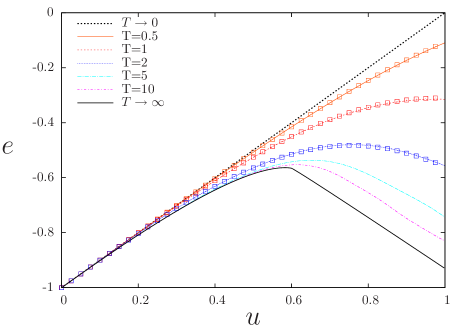
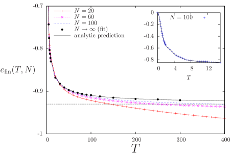
IV.5.3 The long time limit of the annealing towards the paramagnet

Let us now discuss the behavior of the final energy density for large values of $T$ (yet finite with respect to $N$). We expect that this large $T$ limit matches the small $\tau$ limit of the exponentially large time regime studied in Sec. IV.4.3, namely that

$$\lim_{T\to\infty}e_{\textrm{fin}}(T)=\lim_{\tau\to 0}e_{\textrm{fin}}(\tau)=\hat{e}_{\textrm{fin}}\ .$$ (110)

In other words we do not foresee an intermediate scaling regime, as far as the energy density is concerned, between the constant times and the exponentially large times regimes.

The intuitive explanation of this statement, in terms of the gap structure in the spectrum of the quantum Hamiltonian, is the following. The gaps encountered on the metastable continuation of the ferromagnetic groundstate are exponentially small until the spinodal $u_{\rm sp}=1-s_{\rm sp}$ is reached, thus for any finite $T$ no turning on the crossing paramagnetic states can be performed before $u_{\rm sp}$. Around $u_{\rm sp}$ there are some polynomially small gaps that would need a polynomially growing time $T$ to be resolved. However these gaps do not extend to values of $u$ strictly greater than $u_{\rm sp}$, in the thermodynamic limit. Hence in the limit of large $T$, taken after the thermodynamic limit, the evolution should follow the paramagnetic energy levels that join the spinodal point, and hence lead to a final energy density $\hat{e}_{\textrm{fin}}$.

We shall give now a more quantitative justification of the statement (110), and characterize the asymptotic corrections $e_{\textrm{fin}}(T)-\hat{e}_{\textrm{fin}}$ as $T\to\infty$, by analyzing the classical mechanics problem defined in Eqs. (108,109). The large $T$ limit of these equations corresponds to an adiabatic classical mechanics evolution, and we shall thus use the tools from the theory of classical adiabatic invariants arnold06 ; kerkovian87 . Consider first the phase portraits of the classical Hamiltonian (109), plotted on Fig. 21. For $u\leq u_{\rm sp}$ the classical Hamiltonian has a local minimum in $(q,\widetilde{q})=(q_{*}(u),0)$, where $q_{*}(u)$ is given in terms of the longitudinal magnetization $m_{*}$ of the ferromagnetic state by $q_{*}(u)=\sqrt{1-m_{*}(s=1-u)^{2}}$ ($q_{*}$ is in fact the associated transverse magnetization). The corresponding value of $\mathcal{H}$ is $e_{\rm fm}(s=1-u)$. In consequence the classical mechanics evolution has closed trajectories around this minimum, as can be seen on the first two panels of Fig. 21. The initial condition $q_{T}(0)=\widetilde{q}_{T}(0)=0$ corresponds to this minimum in $u=0$, hence for $T\to\infty$ the evolution follows this moving minimum (with corrections of order $1/T$ that will be discussed below), and reaches the point of coordinates $(q_{\rm sp},0)$ at $u_{\rm sp}$ (we denote $q_{\rm sp}=\sqrt{1-m_{\rm sp}^{2}}=1/\sqrt{p-1}$). At the spinodal reached in $u_{\rm sp}$ the ferromagnetic metastable state disappears; in this context this translates into the absence of such closed trajectories for $u\geq u_{\rm sp}$ (note however that the Hamiltonian is $\pi$-periodic in $\widetilde{q}$), see the two last panels of Fig. 21.

Figure 21: Phase portraits of the classical Hamiltonian (109) for $p=3$; from left to right $u=0.3$, $u=0.57$, $u=u_{\rm sp}=0.6$, $u=0.7$.

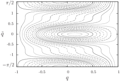
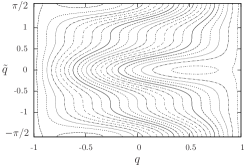
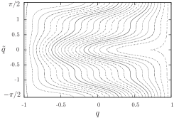
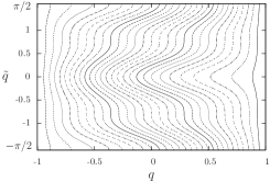
The $T\to\infty$ evolution for $u\geq u_{\rm sp}$ can be understood in terms of classical adiabatic invariants. Let us recall that these are quantities that depend on $(q,\widetilde{q},u)$ and that have small variations along a trajectory solution of Hamilton equations, in the limit where the Hamiltonian of the system has a slow explicit time-dependence with respect to the instantaneous motion of the system, i.e. here in the large $T$ limit. The simplest adiabatic invariant (conserved with corrections of order $T^{-1}$) corresponds to a passage to action-angle variables, and reads

$$\mathcal{I}(q,\widetilde{q},u)=\underset{\mathcal{H}(q^{\prime},\widetilde{q}^{\prime},u)=\mathcal{H}(q,\widetilde{q},u)}{\oint}\widetilde{q}^{\prime}\,{\rm d}q^{\prime}\ ,$$ (111)

where the integral is performed over a trajectory starting in $(q,\widetilde{q})$ that corresponds to Hamiltonian conservative evolution for a fixed value of $u$. Note that in this case the adiabatic invariant depends on $(q,\widetilde{q},u)$ only through $(e,u)$ where $e=\mathcal{H}(q,\widetilde{q},u)$ is the fixed energy on the trajectory. For the lines of the phase portraits that reach the points $\widetilde{q}=\pm\pi/2$, this quantity can be computed by expressing $\widetilde{q}^{\prime}$ as a function of $q^{\prime}$ and $e=\mathcal{H}(q^{\prime},\widetilde{q}^{\prime})$. Inverting the relation (109) one obtains

$$\mathcal{I}(e,u)=2\int_{{q_{\rm min}}(e,u)}^{{q_{\rm max}}(e,u)}\frac{1}{2}\text{acos}\,\left(\left(-\frac{e+uq}{(1-u)(1-q^{2})^{p/2}}\right)^{\frac{1}{p}}\right){\rm d}q^{\prime}\ ,$$ (112)

where ${q_{\rm min}}$ and ${q_{\rm max}}$ denote the extremal points of the trajectory. A moment of thought reveals that for $u\geq u_{\rm sp}$ this quantity is proportional to the integrated density of states ${\cal D}_{0}$: compare it with the expression of ${\cal D}_{0}$ in (44), and the semi-classical solution of the eigenvalue equation expressed in the $x$-basis given in Eq. (42). This shows that the conservation of adiabatic invariants in the $T\to\infty$ limit is strictly equivalent to the iso-density argument used in the analysis of exponentially large timescales. Hence the classical mechanics adiabatic evolution between $u=u_{\rm sp}$ and $u=1$ brings the system to the final energy $\hat{e}_{\textrm{fin}}$, defined by ${\cal D}_{0}(s_{\rm sp},e_{\rm sp})={\cal D}_{0}(0,\hat{e}_{\textrm{fin}})$.

We shall now discuss the behavior of $e_{\textrm{fin}}(T)-\hat{e}_{\textrm{fin}}$ in the large $T$ limit. One can expect some generic corrections of order $T^{-1}$ to arise because of the imperfect conservation of the adiabatic invariant for large but finite $T$. However these effects are subdominant with respect to the singular corrections due to the bifurcation transition of the classical mechanics system at $u_{\rm sp}$ haberman00 . The left panel of Fig. 22 displays the functions $q_{T}(u)$ for several values of $T$. For large enough $T$ they indeed follow with a good approximation $q_{*}(u)$ for $u<u_{\rm sp}$, while they have an oscillating behavior for $u>u_{\rm sp}$, in agreement with the shape of the phase portraits. The critical regime around $u_{\rm sp}$ plays however a crucial role, as will be explained now by reconsidering in a quantitative way the reasoning above.

      

Figure 22: Left: the solutions $q_{T}(u)$ of Eq.(108) for $p=3$, $T=50,100,400$, with their adiabatic limit $q_{*}(u)$ when $u\leq u_{\rm sp}$. Right: similar datas for $T=100,400,800$ plotted with the rescaling defined in Eq. (119), together with the tritronquée solution of the Painlevé equation.

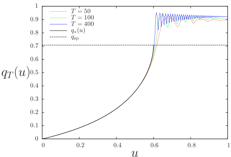
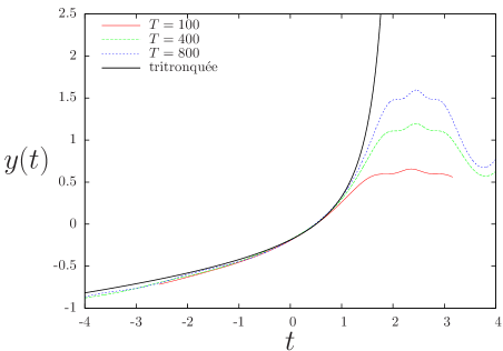
For $u<u_{\rm sp}$, the expansion of the Hamiltonian (109) around its minimum in $(q,\widetilde{q})=(q_{*}(u),0)$ yields

$$\mathcal{H}(q,\widetilde{q},u)=e_{\rm fm}(s=1-u)+\frac{1}{2}g(u)\omega(u)^{2}(q-q_{*}(u))^{2}+\frac{1}{2g(u)}\widetilde{q}^{2}+O((q-q_{*}(u))^{3},\widetilde{q}^{4},(q-q_{*}(u))\widetilde{q}^{2})\ ,$$ (113)

which corresponds to an harmonic oscillator centered in $q_{*}(u)$, with mass and pulsation given by

$$g(u)=\frac{1}{4p(1-u)(1-q_{*}(u)^{2})^{p/2}}\ ,\quad\omega(u)=2p(1-u)(1-q_{*}(u)^{2})^{\frac{p}{2}-1}\sqrt{1-(p-1)q_{*}(u)^{2}}\ .$$ (114)

In the large $T$ limit one can set up an expansion for the trajectory of an harmonic oscillator with slowly varing parameters (here $q_{*},g,\omega$), under the form of oscillating terms of pulsation $T\omega(u)$ (in the slow time $u$) multiplied by slowly varying terms. At the leading order, and taking into account the initial condition $q_{T}(0)=\widetilde{q}_{T}(0)=0$, one obtains

$$q_{T}(u) = q_{*}(u)-\frac{1}{T}q_{*}^{\prime}(0)\sqrt{\frac{g(0)}{\omega(0)g(u)\omega(u)}}\sin\left(T\int_{0}^{u}{\rm d}u^{\prime}\,\omega(u^{\prime})\right)+O(T^{-2})\ ,$$ (115)

$$\widetilde{q}_{T}(u) = \frac{1}{T}g(u)q_{*}^{\prime}(u)-\frac{1}{T}q_{*}^{\prime}(0)\sqrt{\frac{g(0)g(u)\omega(u)}{\omega(0)}}\cos\left(T\int_{0}^{u}{\rm d}u^{\prime}\,\omega(u^{\prime})\right)+O(T^{-2})\ .$$ (116)

This expansion is only valid for $u<u_{\rm sp}$, because $\omega(u)$ vanishes as $u\to u_{\rm sp}$. In this limit the harmonic potential is not confining anymore. To continue the description of the evolution towards larger values of $u$ we shall now expand the Hamiltonian around its bifurcation, and look for a scaling function that will describe the neighborhood of the singularity. We write:

$$\mathcal{H}(q,\widetilde{q},u)=e_{\rm sp}-e^{\prime}_{\rm fm}(s_{\rm sp})(u-u_{\rm sp})+\frac{1}{2g(u_{\rm sp})}\widetilde{q}^{2}-\frac{1}{3!}a_{p}(q-q_{\rm sp})^{3}-b_{p}(q-q_{\rm sp})(u-u_{\rm sp})+\dots\ ,$$ (117)

where $a_{p}$ and $b_{p}$ are two positive constants depending on $p$ that can be obtained as partial derivatives of $\mathcal{H}$ in $(q_{\rm sp},0,u_{\rm sp})$. The mechanical interpretation of the last three terms is a particle of mass $g(u_{\rm sp})$, evolving in an energy potential that has a constant cubic term and a linear term whose sign changes as $u$ crosses $u_{\rm sp}$, thus provoking the disappearance of its stable minimum. Eliminating $\widetilde{q}$ from the Hamilton equations of motion that follows from this truncated expansion leads to

$$\frac{1}{T^{2}}\frac{{\rm d}^{2}}{{\rm d}u^{2}}(q_{T}(u)-q_{\rm sp})=\frac{a_{p}}{2g(u_{\rm sp})}(q_{T}(u)-q_{\rm sp})^{2}+\frac{b_{p}}{g(u_{\rm sp})}(u-u_{\rm sp})\ .$$ (118)

We define a scaling function $y(t)$ with

$$\begin{cases}y=T^{2/5}\,C_{p}^{(y)}\,(q-q_{\rm sp})\ ,\qquad C_{p}^{(y)}=\frac{g(u_{\rm sp})}{b_{p}}\left(\frac{a_{p}b_{p}}{12g(u_{\rm sp})^{2}}\right)^{3/5}\ ,\\ t=T^{4/5}\,C_{p}^{(t)}\,(u-u_{\rm sp})\ ,\qquad C_{p}^{(t)}=\left(\frac{a_{p}b_{p}}{12g(u_{\rm sp})^{2}}\right)^{1/5}=\frac{\left(\frac{8}{3}\right)^{\frac{1}{5}}p^{\frac{3}{5}}\frac{(p-2)^{\frac{3p-4}{10}}}{(p-1)^{\frac{3p-5}{10}}}}{\left(1+p\frac{(p-2)^{\frac{p-2}{2}}}{(p-1)^{\frac{p-1}{2}}}\right)^{\frac{2}{5}}}\ .\end{cases}$$ (119)

The scalings with $T$ of these changes of variables are chosen in such a way that the three terms of Eq. (118) are of the same order. The constants $C_{p}^{(y)}$ and $C_{p}^{(t)}$ are more arbitrary, and have been chosen here in order for the scaling function $y(t)$ to be solution of the canonical form of the first Painlevé equation, $y^{\prime\prime}(t)=6\,y(t)^{2}+t$. We have only given $C_{p}^{(t)}$ explicitly above as $C_{p}^{(y)}$ will not appear in the final result. There exists of course an infinite family of solutions of the Painlevé equation, selected for instance by the value of $(y,y^{\prime})$ at a given $t$. In our case the solution will be selected by a matching argument between the $u\to u_{\rm sp}$ limit of the first regime $u<u_{\rm sp}$ described by Eq. (115), and the $t\to-\infty$ limit of the regime described by the Painlevé equation (in a neighborhood of $u_{\rm sp}$ of order $T^{-4/5}$). To expand Eq. (115) we note that in the limit $u\to u_{\rm sp}$ one has $q_{*}(u)=q_{\rm sp}-\sqrt{2b_{p}(u_{\rm sp}-u)/a_{p}}+O((u_{\rm sp}-u)^{3/2})$ and $\omega(u)\sim\text{cst}\,(u_{\rm sp}-u)^{1/4}$, where here and in the following we denote cst positive constants whose precise values are not necessary for the reasoning. These expansions yields, in terms of the rescaled variables $y$ and $t$,

$$y(t)\underset{t\to-\infty}{\sim}-\sqrt{\frac{-t}{6}}-\text{cst}\ T^{-1/2}(-t)^{-1/8}\sin(T(\text{cst}-\text{cst}\,(-t)^{5/4}))\ .$$ (120)

The leading term $-\sqrt{-t/6}$ is common to several solutions of the first Painlevé equation; however we note here that the amplitude of the oscillating term vanishes as $T\to\infty$ (for a fixed large $t$), hence the scaling function should be given by a monotonous solution with the $-\sqrt{-t/6}$ asymptotic behaviour. This was shown in Joshi2001 to imply that $y(t)$ is Boutroux boutroux tritronquée solution. This solution was studied in great details in Joshi2001 , in particular the location of its smallest real pole $t_{0}$ was determined numerically with great accuracy, and found to be $t_{0}=2.3841687\dots$. On the right panel of Fig. 22 we compare the tritronquée solution of the Painlevé equation (determined numerically with its values $(y(0),y^{\prime}(0))$ given in Joshi2001 ) with the curves $q_{T}(u)$, rescaled according to (119). Their agreement improves as $T$ increases, as expected for a scaling function. One can compute the instantaneous energy in the regime described by the Painlevé equation, namely for $u\sim u_{\rm sp}+T^{-4/5}t/C_{p}^{(t)}$ with $t<t_{0}$, and find from (117) that it is given by $e_{\rm sp}-e^{\prime}_{\rm fm}(s_{\rm sp})(u-u_{\rm sp})+O(T^{-6/5})$. Let us also compute the integrated density of states associated to such energies,

$${\cal D}_{0}\left(s=s_{\rm sp}-T^{-4/5}\frac{t}{C_{p}^{(t)}},e=e_{\rm sp}-e^{\prime}_{\rm fm}(s_{\rm sp})T^{-4/5}\frac{t}{C_{p}^{(t)}}\right)\sim{\cal D}_{0}(s_{\rm sp},e_{\rm sp})+M_{p}T^{-4/5}\frac{t}{C_{p}^{(t)}}\ ,$$ (121)

where $M_{p}$ was defined explicitly in Eq. (98). As explained above the conservation of mechanical classical invariants corresponds to the conservation of the integrated density of states for $u\geq u_{\rm sp}$. Our prediction for the large $T$ behaviour of the final energy density thus reads

$$e_{\textrm{fin}}(T)\sim\hat{e}_{\textrm{fin}}+2M_{p}\frac{t_{0}}{C_{p}^{(t)}}T^{-4/5}\ .$$ (122)

Indeed the largest violation of the conservation of the adiabatic invariant is obtained by taking $t\to t_{0}$, the limit of existence of the scaling regime described by the Painlevé equation.

It is rather peculiar that a scaling function matching two different regimes is defined only on a part of the real axis (here $t<t_{0}$). In fact at the end of the Painlevé regime the values of $u$ are still close to the singularity ($u-u_{\rm sp}=O(T^{-4/5})$), hence the periods of the orbits encountered at those times are divergent. It has been shown in haberman00 how to deal with this third regime of time, that matches the $t\to t_{0}$ limit with $u=u_{\rm sp}+\varepsilon$, where $\varepsilon$ is arbitrary small but independent on $T$. In particular it was found that the additional corrections to the adiabatic invariant due to this regime are of order $T^{-5/6}$, i.e. asymptotically neglectible with respect to those we have computed, yet larger than the regular $T^{-1}$ corrections to the action adiabatic invariant.

We have checked the analytical prediction (122) against numerical integrations of the Hamilton equations of motion, and present these results on Fig. 23. We could not achieve a good agreement with the data using only the form (122); indeed, even for the largest times $T=24000$ we could reach, the subdominant correction term of order $T^{-5/6}$ haberman00 is comparable to the leading one (the difference between the two exponents $4/5$ and $5/6$ is tiny). Including this correction term as a fitting parameter yields a very good agreement with the data, that is further improved with the inclusion of the regular $T^{-1}$ corrections. We have also checked for other values of $p$ a similar agreement with the prediction of Eq. (122).

Figure 23: The large $T$ limit of the final energy density for the annealing towards the paramagnet of the $p=3$ model. The symbols have been obtained via the integration of Hamilton equation of motion, for $T$ as large as 24000. The two lines are of the form $e_{\textrm{fin}}(T)-\hat{e}_{\textrm{fin}}=a\,T^{-4/5}+b\,T^{-5/6}+c\,T^{-1}$. In both cases $a$ was fixed by the analytical prediction from Eq. (122), the function $f_{1}$ was obtained with $c=0$ and using $b$ as a fitting parameter, while for $f_{2}$ we fitted the data with both $b$ and $c$.

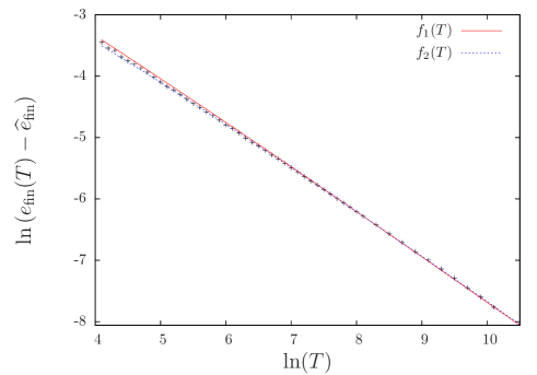
IV.6 Even values of $p$

Let us finally discuss the annealing for even $p$ models that was left aside in the previous discussion. As explained at the end of Sec. III.1 the models with even $p$ enjoy an additional symmetry, the conservation of the parity of the magnetization in the $x$ basis. This implies that the dynamics of the even $p\geq 4$ models has exactly the same properties as the odd $p\geq 3$ cases. Indeed the dynamics is confined to the subspace of parity equal to the one of the groundstate. In that subspace the ferromagnetic levels are unique, and all the structure of the gaps in the spectrum is qualitatively the same as for odd $p\geq 3$ models.

The case $p=2$, studied in santoro08 ; solinas08 ; itin09_1 ; itin09_2 , is on the contrary very different. Consider first the annealing towards the paramagnet. The only relevant timescale, as far as the energy density is concerned, is the one of finite $T$ when $N\to\infty$. Indeed, as explained at the beginning of Sec. IV.5.3, resolving the gaps of order $N^{-1/3}$ encountered around $u_{\rm c}=2/3$ (hence considering interpolation times of order $N^{2/3}$) is necessary only to end up the evolution in the groundstate, not to reach energy densities equal to the one of the groundstate. On the finite $T$ timescale the semi-classical analysis of Sec. IV.5.2 is thus relevant, and allows to cover the full range of energy densities between $e_{\textrm{fin}}(T=0)=0$ and $e_{\textrm{fin}}(T\to\infty)=-1$. Moreover the large $T$ corrections to the energy density are much less singular than for $p\geq 3$, because the bifurcation at $u_{\rm c}$ is of a different type. The scaling regime is described by the second Painlevé equation itin09_1 ; itin09_2 instead of the first one, and this should lead to corrections of the form $e_{\textrm{fin}}(T)\sim-1+\text{cst}/T$.

The annealing towards the $p=2$ ferromagnet has a much richer structure. For all finite $T$, in the thermodynamic limit, the semi-classical analysis of Sec. IV.5.1 predicts that $e_{\textrm{fin}}(T)=0$. Indeed the initial condition $(q_{T}(s=0),\widetilde{q}(s=0))=(0,0)$ is a stationary point of $\mathcal{H}$ for all values of $s$, even though it becomes unstable for $s\geq s_{\rm c}$. Reaching non-trivial final energy densities thus requires interpolation time-scales that grows with $N$; their precise scaling is a delicate problem that we leave for future work. Indeed a preliminary treatment, within the formalism of this paper, reveals that the gaps that close along the line $e=-(1-s)$ (corresponding thermodynamically to the unstable solution $m=0$ of Eq. (11)) do so as $1/\ln N$, and not polynomially in $N$ as happens for the groundstate. Such a logarithmic behaviour was already discussed in HeScGe05 ; RiPa09 .

V Conclusions

Let us give a partial summary of this work and propose a few directions for future research. One of our main results in the statics part of the paper is the formula (62) that gives the exponential rate of closing of the gap at a first-order phase transition (i.e. for $p\geq 3$ in this class of models), under the form of a semi-classical tunneling amplitude between the paramagnetic and ferromagnetic states that cross at the transition. At a second-order phase transition (here for $p=2$) we recover the results of botet83 ; dusuel04 on the polynomial scaling $N^{-1/3}$ of the gap, from a matching between the square-root closing of the finite gap in the paramgnetic phase (see Sec. III.6) and the behavior of the exponential splitting of the two ferromagnetic groundstates around the transition (studied in Sec. III.7.2).

The detailed description of the spectral properties of the models studied here, in particular the density of states and the rate of closing of exponentially small gaps, relies on the analysis of the solutions of the semi-classical eigenvalue equation (28). It is actually straightforward to write its generalization, and thus to perform the same subsequent steps of analysis, for any model of spins whose Hamiltonian only depend on the total magnetizations $\widehat{m}^{x},\widehat{m}^{y},\widehat{m}^{z}$. For concreteness let us give these generalizations for three examples:

• In the LMG model the Hamiltonian reads $\widehat{H}/N=-\Gamma\widehat{m}^{z}-\gamma_{x}(\widehat{m}^{x})^{2}-\gamma_{y}(\widehat{m}^{y})^{2}$, and the generalization of (28) is

  $$e=-\Gamma\,m-\gamma_{x}(1-m^{2})\cosh^{2}(2\varphi^{\prime}(m))+\gamma_{y}(1-m^{2})\sinh^{2}(2\varphi^{\prime}(m))\ .$$ (123)

  For the density of states this should yield formulas equivalent to those obtained in ribeiro08 .

• For the models of FiDuVi11 , where the interactions along two axis are raised to arbitrary powers, one can write the Hamiltonian as $\widehat{H}/N=-\gamma_{z}(\widehat{m}^{z})^{p}-\gamma_{x}(\widehat{m}^{x})^{p^{\prime}}$ and the eigenvalue equation, in the thermodynamic limit, as

  $$e=-\gamma_{z}\,m^{p}-\gamma_{x}(1-m^{2})^{\frac{p^{\prime}}{2}}\cosh(2\varphi^{\prime}(m))^{p^{\prime}}\ .$$ (124)

• The authors of SeNi12 introduced an antiferromagnetic coupling in the interpolating Hamiltonian of the annealing, under the form $\widehat{H}/N=-s[\lambda(\widehat{m}^{z})^{p}-(1-\lambda)(\widehat{m}^{x})^{2}]-(1-s)\widehat{m}^{x}$. This yields

  $$e=-s\lambda m^{p}+s(1-\lambda)(1-m^{2})\cosh(2\varphi^{\prime}(m))^{2}-(1-s)\sqrt{1-m^{2}}\cosh(2\varphi^{\prime}(m))\ .$$ (125)

In the Section IV devoted to the annealing dynamics of the fully-connected $p$-spin models we have analyzed the final energy density $e_{\textrm{fin}}$ after an evolution on a time $T$. Our analytical results have been obtained in the thermodynamic limit; let us emphasize the necessity, in this limit, to define precisely the scaling of $T$ with the system size $N$. The results, and the methods employed to derive them, are indeed very different according to the timescale investigated. In Sec. IV.4 we studied annealing times $T$ growing exponentially with $N$, in terms of the Landau-Zener mechanism controlled by the exponentially small gaps encountered by metastable states. The regime where $T$ is kept fixed while the limit $N\to\infty$ is performed first was analyzed in Sec. IV.5, via a reduction to a classical mechanics problem sciolla11 . We have argued that these two regimes are the only relevant ones for $p\geq 3$, and as far as the energy density is concerned; resolving finite (extensive) energy differences would require in some cases the study of an intermediate timescale, with $T$ growing polynomially or logarithmically with $N$. An outcome of our analysis is the crucial role played by spinodals in the annealing of mean-field models encountering a first-order transition: in the limit where $T$ is large but finite with respect to $N$, or exponential with $N$ but with an infinitesimal growth rate $\tau$, an annealing follows the metastable groundstate until its disappearance at the spinodal, and reaches at the end of the evolution an excited energy density $\hat{e}_{\textrm{fin}}$ corresponding to the state that crosses the metastable state at the spinodal. This energy separates what can be achieved on sub-exponential times ($e\geq\hat{e}_{\textrm{fin}}$), from the range of energies $e_{\rm gs}\leq e_{\textrm{fin}}\leq\hat{e}_{\textrm{fin}}$ that require an exponentially large annealing time to be reached. In the models studied here the paramagnetic state is always metastable and has no spinodal, hence the annealing from the paramagnet has a trivial finite-time regime ($\hat{e}_{\textrm{fin}}=0$); this motivated the complementary study of the annealing in the reverse direction (from the ferromagnet to the paramagnet) which exhibits a non-trivial boundary $\hat{e}_{\textrm{fin}}$ between the two timescales.

As we already emphasized the models studied in this paper are only toy-models as far as the difficulty of finding their groundstates is concerned; from this point of view both directions of the annealing (from the paramagnet to the ferromagnet or viceversa) are equally relevant. We conjecture that some of the results we obtained may remain true for the quantum annealing of more difficult combinatorial optimization problems as those of qXOR ; young10 . In particular the scalings of the final energy density for the small $\tau$ limit of exponentially large time-scales (see Eq. (99)) and for the large $T$ limit of constant timescales (see Eq. (122)) with the exponent $4/5$ could be generic for all mean-field models encountering a first-order transition followed by a separate spinodal along their quantum annealing (the location of the spinodals for the XORSAT problem were determined in qXOR ), be there fully-connected or diluted, as long as they are mean-field. Indeed in these combinatorial optimization problems the paramagnetic state from which one starts the annealing procedure has a spinodal limit of existence (exactly as the ferromagnetic state of the toy models studied in the present paper). One of the several open questions in this context would be the determination of $\hat{e}_{\textrm{fin}}$, in other words the generalization of the iso-integrated density argument that applies only to the fully-connected models whose Hilbert space can be decomposed in disconnected spin sectors. One possible road for this calculation in the context of diluted mean-field models would be the quantum extension of the “state following method” ZdKr10 (related to the Franz-Parisi potential FrPa95 ), that answers a similar question for classical annealing dynamics.

In the design of a quantum annealing algorithm there is some freedom in the choice of the initial Hamiltonian $\widehat{H}_{\rm i}$ (it should however have a groundstate that is easy to prepare, and its construction should not assume a detailed knowledge of the sought-for groundstate of the final Hamiltonian $\widehat{H}_{\rm f}$). To avoid the phase transitions that appear when $\widehat{H}_{\rm i}$ is a transverse field it was for instance proposed in farhi_random to randomize the direction of the transverse fields on each spin. Very recently another proposal was to include antiferromagnetic couplings in the interpolating Hamiltonian SeNi12 ; in this way it is possible to avoid the first-order phase transition by making a detour in the $(s,\lambda)$ plane (see also ribeiro06 for a similar phenomenon). The annealing towards the ferromagnet for $p\geq 3$ studied in the paper was particularly inefficient because the groundstate of the initial Hamiltonian (the transverse field $-\widehat{m}^{x}$) remained metastable all the way to $s=1$. One can thus wonder whether taking a ferromagnetic coupling $-(\widehat{m}^{x})^{p^{\prime}}$ with $p^{\prime}\geq 2$ (this corresponds to the models of FiDuVi11 ) would help. The answer is no, the metastability until $s=1$ persists for all values of $p^{\prime}$, as long as $p\geq 3$. Instead the antiferromagnetic coupling $(\widehat{m}^{x})^{2}$ introduced in SeNi12 helps the annealing because their groundstate $|0;0\rangle_{x}$ has a much larger overlap with the groundstate $|1;0\rangle_{z}$ of the target Hamiltonian $-(\widehat{m}^{z})^{p}$ than has the groundstate $|1;0\rangle_{x}$ of the transverse field.

In the fully-connected ferromagnetic models studied in this paper the condition for a thermodynamic first-order transition (i.e. $p\geq 3$) coincided with the existence of exponentially small gaps at the transition. There can however be exceptions to this rule: the case $p=p^{\prime}=2$ of FiDuVi11 exhibits a discontinuity in the derivative of the groundstate energy but no exponentially small gaps. This peculiarity is due to the coincidence of the spinodals with the first-order transition, the states that cross become unstable right after the transition. A similar situation was shown to happen in antiferromagnetic chains of odd lenghts with periodic boundary conditions LaMoScSo12 .

Appendix A Large $p$ expansion of the closing rate of the gap

This appendix is devoted to the derivation of the asymptotic expansion (63) for the rate of the exponential closing of the gap at the first-order transition, in the large $p$ limit. Let us first compute the limit of $\alpha_{p}$. Simplifying the expression (62) with ${m_{\rm c}}=1$, $s_{\rm c}=1/2$, ${e_{\rm c}}=-1/2$, one obtains:

$$\alpha_{p}\to\frac{1}{2}\int_{0}^{1}{\rm d}m\,\text{ach}\,\left(\frac{1}{\sqrt{1-m^{2}}}\right)=\frac{1}{2}\int_{0}^{1}{\rm d}m\,\arg\tanh(m)=\frac{\ln 2}{2}\ ,$$ (126)

as argued for in jorg10 . For the computation of $\alpha_{p}$ at order $1/p$ the corrections to ${m_{\rm c}}$ and $s_{\rm c}$ given in Eq. (15) are actually irrelevant and one has:

$$\begin{split}\alpha_{p}&=\frac{1}{2}\int_{0}^{1}{\rm d}m\,\text{ach}\,\left(\frac{1}{\sqrt{1-m^{2}}}\left(1-m^{p}\right)\right)+O\left(\frac{1}{p^{2}}\right)\\ &=\frac{1}{2}\sum_{k=0}^{\infty}\frac{1}{k!}\int_{0}^{1}{\rm d}m\,\left(\frac{-m^{p}}{\sqrt{1-m^{2}}}\right)^{k}\left(\frac{{\rm d}}{{\rm d}^{k}}\text{ach}\,\right)\left(\frac{1}{\sqrt{1-m^{2}}}\right)+O\left(\frac{1}{p^{2}}\right)\ .\end{split}$$ (127)

In general one has $\frac{{\rm d}}{{\rm d}^{k}}\text{ach}\,x=\sum_{i=\frac{k+1}{2}}^{k-1}c_{i,k}\frac{x^{2i-(k+1)}}{(x^{2}-1)^{i-1/2}}$, and therefore the $k-$th integral above is found to be:

$$(-1)^{k}\sum_{i}c_{i,k}\int_{0}^{1}{\rm d}m\,m^{kp+1-2i}=\frac{(-1)^{k}}{kp}\sum_{i}c_{i,k}+O\left(\frac{1}{p^{2}}\right)=\frac{-(k-1)!}{kp}+O\left(\frac{1}{p^{2}}\right)\ ,$$ (128)

where we used that $\sum_{i}c_{i,k}=\lim_{x\rightarrow\infty}x^{k}\frac{{\rm d}^{k}}{{\rm d}x^{k}}\text{ach}\,(x)=\lim_{x\rightarrow\infty}x^{k}\frac{d^{k}}{dx^{k}}\ln x=(-1)^{k-1}(k-1)!x^{-k}$. We obtain finally the expansion of Eq. (63):

$$\begin{split}\alpha_{p}&=\frac{\ln 2}{2}-\frac{1}{2p}\sum_{k=1}^{\infty}\frac{(k-1)!}{k.k!}+O\left(\frac{1}{p^{2}}\right)\\ &=\frac{\ln 2}{2}-\frac{1}{2p}\sum_{k=1}^{\infty}\frac{1}{k^{2}}+O\left(\frac{1}{p^{2}}\right)=\frac{\ln 2}{2}-\frac{\pi^{2}}{12p}+O\left(\frac{1}{p^{2}}\right)\ .\end{split}$$ (129)

Appendix B Technical details on the simplified model

B.1 Statics

We justify in this appendix the formula (85) for the rate of closing of the gaps of the simplified model, along the metastable continuation of its groundstate for $s\geq 1/2$. We look for an eigenvector of $\widehat{H}_{\bullet}(s)$, with an eigenvalue $Ne$, under the form $\underset{m\in{{\cal M}^{N}_{0}}}{\sum}\phi(m,s,e)|m;0\rangle_{x}$. The coefficients of this decomposition are solutions of

$$e\,\phi(m,s,e)=-sm\phi(m,s,e)-(1-s)D_{m}\sum_{m^{\prime}\in{{\cal M}^{N}_{0}}}D_{m^{\prime}}\phi(m^{\prime},s,e)\ .$$

For $s=0$ the lowest eigenstate is given exactly by $\phi(m,0,-1)=D_{m}$, which can be written at the leading order in the thermodynamic limit $e^{-N\varphi_{0}(m)}$, with $\varphi_{0}$ given in Eq. (34). For $0\leq s<1/2$ we construct an approximation $\phi(m,s)$ of the groundstate eigenvector as

$$\phi(m,s)=\frac{\widetilde{\phi}(m,s)}{\|\widetilde{\phi}(s)\|}\ ,\qquad\text{with}\ \ \widetilde{\phi}(m,s)=\frac{\phi(m,0,-1)}{1-\frac{s}{1-s}m}\ .$$ (130)

Indeed one has :

$$\begin{split}-\left(1-\frac{s}{1-s}m\right)\phi(m,s)=-\frac{\phi(m,0,-1)}{\|\widetilde{\phi}(s)\|}&=-D_{m}\sum_{m^{\prime}\in{{\cal M}^{N}_{0}}}D_{m^{\prime}}\frac{\phi(m^{\prime},0,-1)}{\|\widetilde{\phi}(s)\|}\\ &=-D_{m}\sum_{m^{\prime}\in{{\cal M}^{N}_{0}}}D_{m^{\prime}}\phi(m^{\prime},s)+O\left(\frac{\phi(m,s)}{\sqrt{N}}\right)\ .\end{split}$$ (131)

Thus :

$$-(1-s)\phi(m,s)=-sm\phi(m,s)-(1-s)D_{m}\sum_{m^{\prime}\in{{\cal M}^{N}_{0}}}D_{m^{\prime}}\phi(m^{\prime},s)+O\left(\frac{\phi(m,s)}{\sqrt{N}}\right)\ .$$ (132)

This shows that, for $s<1/2$, the groundstate has energy close to $-(1-s)$ and takes the form

$$\phi(m,s,-(1-s))=e^{-N\varphi_{0}(m)+O(\sqrt{N})}\ .$$ (133)

For $s\geq 1/2$, there appears a divergence in the definition of $\phi(m,s)$ at $m=\frac{1-s}{s}$, a sign of the avoided crossing with an eigenvector localized near $m=\frac{1-s}{s}$ in the $x$-basis. This divergence is lifted by constructing the symmetric and antisymmetric combinations of these two quasi-eigenvectors. Let $\phi_{\pm}(m,s)=\frac{1}{\sqrt{2}}\left((1-\delta_{m,\frac{1-s}{s}})\phi(m,s)\pm\delta_{m,\frac{1-s}{s}}\right)$. Then one can see that $\phi_{\pm}$ still satisfies (131), and thus correspond to two quasi-eigenvectors at the location of the avoided crossing. At the leading exponential order the gap between the two eigenstates that crosses for some value of $s$ is given by the overlap between the metastable state of eigenvector close to $e^{-N\varphi_{0}(m)}$ and the localized state in $m_{0}(s)=\frac{1-s}{s}$. As a consequence $\gamma_{\bullet}(s)=\varphi_{0}((1-s)/s)$, which explains the origin of Eq. (85).

B.2 Annealing with a sub-exponential interpolation time

In this appendix we present an analysis of the annealing of the simplified model with an interpolation time growing sub-exponentially with $N$. The Schrödinger equation on the vector $|\phi_{T}(s)\rangle=\underset{m\in{{\cal M}^{N}_{0}}}{\sum}\phi_{T}(m,s)|m;0\rangle_{x}$ reads :

$$\frac{i}{T}\frac{{\rm d}\phi_{T}(m,s)}{{\rm d}s}=-sNm\phi_{T}(m,s)-N(1-s)D_{m}\sum_{m^{\prime}\in{{\cal M}^{N}_{0}}}D_{m^{\prime}}\phi_{T}(m^{\prime},s)=-sNm\phi_{T}(m,s)-N(1-s)f_{T}(s)\ ,$$ (134)

where we introduced $f_{T}(s)=\underset{m\in{{\cal M}^{N}_{0}}}{\sum}D_{m}\phi_{T}(m,s)$. By summing (134) over $m$ we obtain:

$$\frac{i}{T}\frac{{\rm d}f_{T}(s)}{{\rm d}s}=-sN\langle m\rangle_{s,T}-N(1-s)f_{T}(s)$$ (135)

with $\langle m\rangle_{s,T}=\underset{m\in{{\cal M}^{N}_{0}}}{\sum}mD_{m}\phi_{T}(m,s)$. Note that $\langle m\rangle_{s=0,T}=0$. Assume first that one can neglect $\langle m\rangle_{s,T}$ in (135). Then using the initial value $f_{T}(0)=1$, one obtains $f_{T}(s)=e^{iNT(s-s^{2}/2)}$. Replacing into (134) gives:

$$\frac{i}{T}\frac{{\rm d}\phi_{T}(m,s)}{{\rm d}s}=-sNm\phi_{T}(m,s)-N(1-s)e^{iNT(s-s^{2}/2)}\ .$$ (136)

A solution of the associated homogenous equation is $\phi_{T}^{({\rm h})}(m,s)=e^{iTs^{2}Nm/2}$. Writing the solution of the complete equation (136) as $\phi_{T}(m,s)=\lambda_{T}(m,s)\phi_{T}^{({\rm h})}(m,s)$ leads to:

$$\frac{i}{T}\frac{{\rm d}\lambda_{T}(m,s)}{{\rm d}s}=-N(1-s)e^{\frac{-iTs^{2}Nm}{2}}e^{iNT\left(s-s^{2}/2\right)}\ ,$$ (137)

with $\lambda_{T}(m,s=0)=D_{m}$. Let us now write $\lambda_{T}(m,s)=h_{N,T}(m,s)e^{Ng_{T}(m,s)}$, and assume that $\underset{N\to\infty}{\lim}\frac{1}{N}\ln\frac{{\rm d}g_{T}(m,s)}{{\rm d}s}=0$ and $\underset{N\to\infty}{\lim}\frac{1}{N}\ln h_{N,T}(m,s)=0$. Then it is easily found that $g_{T}(m,s)=-\varphi_{0}(m)-iTs^{2}m/2+iT(s-s^{2}/2)$, and thus $\phi_{T}(m,s)=\phi_{T}(m,s=0)h_{N,T}(m,s)f_{T}(s)$. The two conditions above then reduces to $\lim_{N\to\infty}\frac{1}{N}\ln T=0$, that is, that one considers sub-exponential times. Finally, it is easy to check that in this regime $\langle m\rangle_{s,T}=0$, and thus that our derivation is indeed self-consistent.

To summarize, in this case, $\phi_{T}(m,s)$ is up to subdominant corrections equal to $\phi_{T}(m,0)$ times a phase independent on $m$, and the final energy $e_{\textrm{fin}}(T)$ is thus identically zero. Therefore we showed that for the simplified model:

$$\sup_{a}\lim_{T,N\to\infty}e_{\textrm{fin}}(T=N^{a},N)=\lim_{T\rightarrow\infty}e_{\textrm{fin}}(T)=\lim_{\tau\rightarrow 0}e_{\textrm{fin}}(\tau)=0\ ,$$ (138)

where the last term comes from the analysis of (small) exponential times of Sec. IV.4.1.

Appendix C Numerical integration of the Schrödinger equation

In this appendix we explain the details of the procedure we used for the numerical treatment of the finite $N$ dynamics, inspired by huyg90 ; poulin11 . Solving the time-dependent Schrödinger equation (75) amounts to compute the evolution operator $\mathcal{U}(0,1)=\mathcal{T}\left(e^{-iT\int_{0}^{1}\widehat{H}(s){\rm d}s}\right)$ where $\mathcal{T}$ denotes the time-ordering operation. It is convenient numerically to break the time interval $s\in[0,1]$ in $n$ intervals of length $\Delta s=1/n$, with equidistant discrete times $s_{i}=(i-1)/n$. This allows to write:

$$\mathcal{U}(0,1)=\mathcal{T}\left(e^{-iT\int_{0}^{1}\widehat{H}(s){\rm d}s}\right)=\prod_{i=1}^{n}\mathcal{T}\left(e^{-iT\int_{s_{i}}^{s_{i+1}}\widehat{H}(s){\rm d}s}\right)=\prod_{i=1}^{n}\mathcal{U}(s_{i},s_{i+1})\ .$$ (139)

We are interested in the particular case of a linear dependency of $\widehat{H}(s)$ on $s$: $\widehat{H}(s)=(1-s)\widehat{H}_{\rm i}+s\widehat{H}_{\rm f}$. The approximation

$$\begin{split}\mathcal{U}(s,s+\Delta s)=\mathcal{T}\left(e^{-iT\int_{s}^{s+\Delta s}\widehat{H}(s^{\prime}){\rm d}s^{\prime}}\right)\rightarrow&\left(e^{-iT\int_{s}^{s+\Delta s}s^{\prime}\widehat{H}_{\rm f}{\rm d}s^{\prime}}\right)\left(e^{-iT\int_{s}^{s+\Delta s}(1-s^{\prime})\widehat{H}_{\rm i}{\rm d}s^{\prime}}\right)\\ &=\left(e^{-iT\frac{2s\Delta s+\Delta s^{2}}{2}\widehat{H}_{\rm f}}\right)\left(e^{-iT\frac{2(1-s)\Delta s-\Delta s^{2}}{2}\widehat{H}_{\rm i}}\right)\\ &\equiv\widetilde{\mathcal{U}}_{\Delta s}(s)\end{split}$$ (140)

gives rise to an error in operator norm $\|A\|\equiv\sup_{X,\|X=1\|}\|AX\|$ bounded by huyg90 :

$$\|\mathcal{U}(s,s+\Delta s)-\widetilde{\mathcal{U}}_{\Delta s}(s)\|\leq\|[\widehat{H}_{\rm i},\widehat{H}_{\rm f}]\|\frac{T(\Delta s)^{2}}{2}+O(\Delta s^{3})=O(NT\Delta s^{2})\ .$$ (141)

Indeed in all the cases of interest here the commutator of the initial and final Hamiltonian has a norm of order $N$. We define the approximate evolution operator $\widetilde{\mathcal{U}}(0,s_{i})\equiv\prod_{j=0}^{i-1}\widetilde{\mathcal{U}}_{\Delta s}(s_{j})$. The triangle inequality

$$\begin{split}\|\mathcal{U}(0,s_{i+1})-\widetilde{\mathcal{U}}(0,s_{i+1})\|&=\|\mathcal{U}(0,s_{i})(\mathcal{U}(s_{i},s_{i+1})-\widetilde{\mathcal{U}}_{\Delta s}(s_{i}))+(\mathcal{U}(0,s_{i})-\widetilde{\mathcal{U}}(0,s_{i}))\widetilde{\mathcal{U}}_{\Delta s}(s_{i})\|\\ &\leq\|\mathcal{U}(s_{i},s_{i}+\Delta s)-\widetilde{\mathcal{U}}_{\Delta s}(s_{i})\|+\|\mathcal{U}(0,s_{i})-\widetilde{\mathcal{U}}(0,s_{i})\|\end{split}$$ (142)

leads by recurrence to

$$\|\mathcal{U}(0,1)-\widetilde{\mathcal{U}}(0,1)\|\leq O(nNT\Delta s^{2})=O(NT/n)\ .$$ (143)

One can thus replace the exact evolution operator $\mathcal{U}(0,1)$ by its approximation $\widetilde{\mathcal{U}}(0,1)$ with a precision of order $\epsilon$ in the evaluation of intensive observables if the number of discretization steps $n$ is of order $NT/\epsilon$.

Let us evaluate the total complexity of the procedure. The dynamical evolution occurs in the fully symmetric sector of the Hilbert space, hence all operators are actually matrices of size $N+1$. For the evolution towards the ferromagnet $\widehat{H}_{\rm i}=-N\widehat{m}^{x}$, $\widehat{H}_{\rm f}=-N(\widehat{m}^{z})^{p}$, and we work in the basis where $\widehat{m}^{z}$ is diagonal. We do not compute all the matrix elements of $\widetilde{\mathcal{U}}(0,1)$, but rather its product with the initial state $|\phi_{T}(0)\rangle$, a column vector of size $N+1$. For each time increment $s_{i}\to s_{i+1}$ we have to multiply the (approximation) of $|\phi_{T}(s_{i})\rangle$ by the two matrices in (140). The first multiplication in (140) is computed in a time proportional to $N$ as $\widehat{H}_{\rm f}$ is a diagonal matrix. The multiplication with the second term is performed with $O(N^{2})$ operations, provided $\widehat{m}^{x}$ (whose expression in this basis is given in Eq. 18) is diagonalized as an initialization step (this costs $O(N^{3})$ operations). The total cost of the computation is thus $O(\epsilon^{-1}N^{3}T)+O(N^{3})$. In the exponentially large times regime the second term becomes irrelevant; the limitations of this numerical method arise from the large times investigated rather than from the sizes of the matrices themselves. The evolution towards the paramagnet is treated similarly, the role of $\widehat{H}_{\rm i}$ and $\widehat{H}_{\rm f}$ being simply exchanged with respect to the previous case. The integration of the dynamics of the simplified model defined in Sec. IV.3 is slightly easier. One can indeed exploit the fact that $\widehat{H}_{\rm i}=\widehat{J}$ is a matrix of rank one with its non-zero eigenvalue equal to $-N$, thus

$$e^{a\widehat{J}}=\widehat{1}-\frac{(e^{-aN}-1)}{N}\widehat{J}\ ,$$ (144)

with $\widehat{1}$ the identity matrix. This avoids the diagonalization of the matrix $\widehat{H}_{i}$, and in this case the total complexity of the integration is $O(\epsilon^{-1}N^{2}T)$, the multiplication of a rank one matrix with a vector being computable with $O(N)$ operations.

Appendix D Derivation of Hamilton’s equations of motion

In this Appendix we give some details of the derivation of (104) from (103). A similar computation can be found in sciolla11 .

The equation (103) on $\varphi_{T}(m,s)$ is of the form

$$-\frac{i}{T}\frac{\partial\varphi_{T}(m,s)}{\partial s}=\mathcal{H}\left(m,i\frac{\partial\varphi_{T}(m,s)}{\partial m},s\right)$$ (145)

where $\mathcal{H}(q,\widetilde{q},s)$ is a smooth real function of its parameters. We write $\varphi_{T}(m,s)=g(m,s)-i\theta(m,s)$, with $g$ and $\theta$ real-valued functions (from now on we keep implicit the dependence on $T$). We assume that there exists a continuous function $q(s)$ such that $\frac{\partial g(q(s),s)}{\partial m}=0$ and $\frac{\partial^{2}g(q(s),s)}{\partial m^{2}}\neq 0$ for all times $s$ and we let $\widetilde{q}(s)=\frac{\partial}{\partial m}\theta(q(s),s)$. Then we get:

$$\frac{1}{T}\frac{\partial^{2}g(q(s),s)}{\partial m\partial s}=-\left.\Im\frac{{\rm d}}{{\rm d}m}\mathcal{H}\left(m,i\frac{\partial g}{\partial m}+\frac{\partial\theta}{\partial m},s\right)\right|_{m=q(s)}=-\frac{\partial\mathcal{H}(q(s),\widetilde{q}(s),s)}{\partial\widetilde{q}}\frac{\partial^{2}g(q(s),s)}{\partial m^{2}}\ .$$ (146)

The derivation of the condition $\frac{\partial g(q(s),s)}{\partial m}=0$ with respect to $s$ yields:

$$\frac{1}{T}\frac{{\rm d}q(s)}{{\rm d}s}=-\frac{1}{T}\frac{\frac{\partial^{2}g(q(s),s)}{\partial m\partial s}}{\frac{\partial^{2}g(q(s),s)}{\partial m^{2}}}=\frac{\partial\mathcal{H}(q(s),\widetilde{q}(s),s)}{\partial\widetilde{q}}\ .$$ (147)

In a similar way we obtain:

$$\begin{split}\frac{1}{T}\frac{\partial^{2}\theta(q(s),s)}{\partial m\partial s}&=-\left.\Re\frac{{\rm d}}{{\rm d}m}\mathcal{H}\left(m,i\frac{\partial g}{\partial m}+\frac{\partial\theta}{\partial m},s\right)\right|_{m=q(s)}\\ &=-\frac{\partial\mathcal{H}(q(s),\widetilde{q}(s),s)}{\partial q}-\frac{\partial\mathcal{H}(q(s),\widetilde{q}(s),s)}{\partial\widetilde{q}}\frac{\partial^{2}\theta(q(s),s)}{\partial m^{2}}\ .\end{split}$$ (148)

This leads to

$$\frac{1}{T}\frac{{\rm d}\widetilde{q}(s)}{{\rm d}s}=\frac{1}{T}\frac{\partial^{2}\theta(q(s),s)}{\partial^{2}m}\frac{{\rm d}q(s)}{{\rm d}s}+\frac{1}{T}\frac{\partial^{2}\theta(q(s),s)}{\partial m\partial s}=-\frac{\partial\mathcal{H}(q(s),\widetilde{q}(s),s)}{\partial q}$$ (149)

Therefore $q(s)$ and $\widetilde{q}(s)$ obey indeed Hamilton’s equations of motion for the Hamiltonian $\mathcal{H}(q,\widetilde{q},s)$. Note that the reality condition on $\mathcal{H}$ corresponds to the Hermitianity of the quantum operator $\widehat{H}$, and that the derivation shows also how Eq. (108) is a consequence of Eq. (107).

References

- (1) M. R. Garey and D. S. Johnson, Computers and Intractability, A Guide to the Theory of NP-Completeness (W.H. Freeman and Company, New York, 1979).
- (2) S. Kirkpatrick, C.D. Gelatt, Jr., and M. Vecchi, Science 220, 671 (1983).
- (3) B. Apolloni, N. Cesa-Bianchi, and D. de Falco, Stoc. Proc. Appl. 33, 233 (1989).
- (4) T. Kadowaki and H. Nishimori, Phys. Rev. E 58, 5355 (1998).
- (5) E. Farhi et al., Science 292, 472 (2001).
- (6) G. E. Santoro and E. Tosatti, J. Phys. A: Math. Gen. 39, R393 (2006).
- (7) A. Das and B. K. Chakrabarti (Eds.), Quantum annealing and related optimization methods (Springer-Verlag, Berlin, 2005).
- (8) A. Messiah, Quantum Mechanics, Vol II (Wiley, 1976).
- (9) S. Sachdev, Quantum phase transitions (Cambridge University Press, Cambridge, 2011).
- (10) D. Mitchell, B. Selman, and H. Levesque, Proceedings of the Tenth National Conference on Artificial Intelligence , 459 (1992).
- (11) M. Mézard and A. Montanari, Information, Physics and Computation (Oxford University Press, New York, 2009).
- (12) G. Biroli, R. Monasson, and M. Weigt, Eur. Phys. J. B 14, 551 (2000).
- (13) M. Mézard, G. Parisi, and R. Zecchina, Science 297, 812 (2002).
- (14) F. Krzakala, A. Montanari, F. Ricci-Tersenghi, G. Semerjian, and L. Zdeborova, PNAS 104, 10318 (2007).
- (15) C. Laumann, A. Scardicchio, and S. L. Sondhi, Phys. Rev. B 78, 134424 (2008).
- (16) F. Krzakala, A. Rosso, G. Semerjian, and F. Zamponi, Phys. Rev. B 78, 134428 (2008).
- (17) T. Jörg, F. Krzakala, G. Semerjian, and F. Zamponi, Phys. Rev. Lett. 104, 207206 (2010).
- (18) A. P. Young, S. Knysh, and V. N. Smelyanskiy, Phys. Rev. Lett. 104, 020502 (2010).
- (19) Y. Y. Goldschmidt, Phys. Rev. B 41, 4858 (1990).
- (20) T. M. Nieuwenhuizen and F. Ritort, Physica A 250, 8 (1998).
- (21) G. Biroli and L. F. Cugliandolo, Phys. Rev. B 64, 014206 (2001).
- (22) T. Jörg, F. Krzakala, J. Kurchan, and A. C. Maggs, Phys. Rev. Lett. 101, 147204 (2008).
- (23) J. Dziarmaga, Advances in Physics 59, 1063 (2010).
- (24) V. Vazirani, Approximation algorithms (Springer, Berlin, 2010).
- (25) J. Håstad, Journal of the ACM 48, 798 (2001).
- (26) S. Arora, C. Lund, R. Motwani, M. Sudan, and M. Szegedy, Journal of the ACM 45, 501 (1998).
- (27) D. Aharonov, I. Arad, Z. Landau, and U. Vazirani, Proceedings of the 41st annual ACM symposium on Theory of computing 287, 417 (2009).
- (28) M. Hastings, (2012), arXiv:1201.3387.
- (29) S. Gharibian and J. Kempe, Proc. 26th CCC’11 , 178 (2011).
- (30) R. Botet and R. Jullien, Phys. Rev. B 28, 3955 (1983).
- (31) J. Vidal, R. Mosseri, and J. Dukelsky, Phys. Rev. A 69, 054101 (2004).
- (32) P. Ribeiro and R. Mosseri, Phys. Rev. A 74, 042333 (2006).
- (33) P. Ribeiro, J. Vidal, and R. Mosseri, Phys. Rev. E 78, 021106 (2008).
- (34) T. Jörg, F. Krzakala, J. Kurchan, A. C. Maggs, and J. Pujos, Europhys. Lett. 89, 40004 (2010).
- (35) M. Filippone, S. Dusuel, and J. Vidal, Phys. Rev. A 83, 022327 (2011).
- (36) Y. Seki and H. Nishimori, Phys. Rev. E 85, 051112 (2012).
- (37) T. Caneva, R. Fazio, and G. E. Santoro, Phys. Rev. B 78, 104426 (2008).
- (38) P. Solinas, P. Ribeiro, and R. Mosseri, Phys. Rev. A 78, 052329 (2008).
- (39) A. P. Itin and P. Törmä, (2009), arXiv:0901.4778.
- (40) A. P. Itin and P. Törmä, Phys. Rev. A 79, 055602 (2009).
- (41) J. Vidal, G. Palacios, and C. Aslangul, Phys. Rev. A 70, 062304 (2004).
- (42) A. Das, K. Sengupta, D. Sen, and B. K. Chakrabarti, Phys. Rev. B 74, 144423 (2006).
- (43) B. Sciolla and G. Biroli, J. Stat. Mech. 2011, P11003 (2011).
- (44) P. Ribeiro and T. Paul, Phys. Rev. A 79, 032107 (2009).
- (45) H. Lipkin, N. Meshkov, and A. Glick, Nucl. Phys. 62, 188 (1965).
- (46) L. Chayes, N. Crawford, D. Ioffe, and A. Levit, J. Stat. Phys. 133, 131 (2008).
- (47) R. Brout, K.A. Müller, and H. Thomas, Solid State Communications 4, 507 (1966).
- (48) J. Wilms, J. Vidal, F. Verstraete, and S. Dusuel, J. Stat. Mech. 2012, P01023 (2012).
- (49) W. Fulton and J. Harris, Representation Theory - A First Course (Springer-Verlag, New York, 1991).
- (50) E. Lieb and D. Mattis, J. Math. Phys. 3, 749 (1962).
- (51) B. Nachtergaele, W. Spitzer, and S. Starr, J. Stat. Phys. 116, 719 (2004).
- (52) C. M. Newman and L. S. Schulman, J. Math. Phys. 18, 23 (1977).
- (53) M. Reed and B. Simon, Methods of modern mathematical physics IV : Analysis of Operators (Academic Press, New York, 1978).
- (54) V. V. Ulyanov and O. B. Zaslavskii, Phys. Rep. 216, 179 (1992).
- (55) B. Derrida and G. J. Rodgers, J. Phys. A 26, L457 (1993).
- (56) F. Krzakala, Private communication .
- (57) S. Dusuel and J. Vidal, Phys. Rev. B 71, 224420 (2005).
- (58) L. D. Landau, Physics of the Soviet Union 2, 46 (1932).
- (59) C. Zener, Proceedings of the Royal Society of London 137, 696 (1932).
- (60) A. G. Rojo, arXiv:1004.2914.
- (61) C. Wittig, J. Phys. Chem. B 109, 8428 (2005).
- (62) M. V. Volkov and V. N. Ostrovsky, Phys. Rev. A 75, 022105 (2007).
- (63) N. V. Vitanov and B. M. Garraway, Phys. Rev. A 53, 4288 (1996).
- (64) N. V. Vitanov, Phys. Rev. A 59, 988 (1999).
- (65) G. E. Santoro, R. Marton , E. Tosatti, and R. Car, Science 295, 2427 (2002).
- (66) P. Arbenz, W. Gander, and G. H. Golub, Linear Algebra and its Applications 104, 75 (1988).
- (67) E. Farhi, J. Goldstone, S. Gutmann, and D. Nagaj, International Journal of Quantum Computation 6, 503 (2008).
- (68) L. K. Grover, Phys. Rev. Lett. 79, 325 (1997).
- (69) J. Roland and N. J. Cerf, Phys. Rev. A 65, 042308 (2002).
- (70) M. Schiró and M. Fabrizio, Phys. Rev. Lett. 105, 076401 (2010).
- (71) V. Arnold, V. Kozlov, and A. Neishtadt, Mathematical Aspects of Classical and Celestial Mechanics, Third ed. (Springer, 2006).
- (72) J. Kevorkian, SIAM Review 29, pp. 391 (1987).
- (73) D. C. Diminnie and R. Haberman, Journal of Nonlinear Science 10, 197 (2000).
- (74) N. Joshi and A.V. Kitaev, Studies in Applied Mathematics 107, 253 (2001).
- (75) P. Boutroux, Ann. Ecole Norm. 30, 265 (1913).
- (76) W.D. Heiss, F.G. Scholtz, and H.B Geyer, J. Phys. A: Math. Gen. 38, 1843 (2005).
- (77) L. Zdeborová and F. Krzakala, Phys. Rev. B 81, 224205 (2010).
- (78) S. Franz and G. Parisi, J. Phys. I France 5, 1401 (1995).
- (79) E. Farhi et al., Quantum Information & Computation 11, 181 (2011).
- (80) C.R. Laumann, R. Moessner, A. Scardicchio, and S.L. Sondhi, (2012), arXiv:1202.3646.
- (81) J. Huyghebaert and H. D. Raedt, J. Phys. A 23, 5777 (1990).
- (82) D. Poulin, A. Quarry, R. Somma, and F. Verstraete, Phys. Rev. Lett. 106, 170501 (2011).