\Macro

l2l22,2 \Macrol1l21,2 \Macrol1l11,1 \Macroli∞ \Macrol22 \Macrol11 \Macrol00 \frefformatvario\fancyrefseclabelprefixSection #1 \frefformatvariothmTheorem #1 \frefformatvariolemLemma #1 \frefformatvariocorCorollary #1 \frefformatvariodefDefinition #1 \frefformatvario\fancyreffiglabelprefixFigure #1 \frefformatvario\fancyrefeqlabelprefix(#1) \frefformatvariopropProperty #1 \frefformatvarioexmplExample #1 \frefformatvarioappAppendix #1 \frefformatvario\fancyreftablabelprefixTable #1

Probabilistic Recovery Guarantees
for Sparsely Corrupted Signals

Graeme Pope, , Annina Bracher, and Christoph Studer,  The material in this paper was presented in part at the IEEE Information Theory Workshop (ITW), September, Lausanne, Switzerland, 2012[1].G. Pope and A. Bracher are with the Dept. of Information Technology and Electrical Engineering, ETH Zurich, 8092 Zurich, Switzerland (e-mail: gpope@nari.ee.ethz.ch, brachera@student.ethz.ch). C. Studer is with the Dept. of Electrical and Computer Engineering, Rice University, Houston, TX 77005, USA (e-mail: studer@rice.edu).The work of C. Studer was supported by the Swiss National Science Foundation (SNSF) under Grant PA00P2-134155.
Abstract

We consider the recovery of sparse signals subject to sparse interference, as introduced in Studer et al., IEEE Trans. IT, 2012. We present novel probabilistic recovery guarantees for this framework, covering varying degrees of knowledge of the signal and interference support, which are relevant for a large number of practical applications. Our results assume that the sparsifying dictionaries are characterized by coherence parameters and we require randomness only in the signal and/or interference. The obtained recovery guarantees show that one can recover sparsely corrupted signals with overwhelming probability, even if the sparsity of both the signal and interference scale (near) linearly with the number of measurements.

Index Terms:
Sparse signal recovery, probabilistic recovery guarantees, coherence, basis pursuit, signal restoration, signal separation, compressed sensing.

I Introduction

We consider the problem of recovering the sparse signal vector 𝐱na𝐱superscriptsubscript𝑛𝑎\mathbf{x}\in\mathbb{C}^{{n_{a}}} with support set 𝒳𝒳\mathcal{X} (containing the locations of the non-zero entries of 𝐱𝐱\mathbf{x}) from m𝑚m linear measurements [2]

𝐳=𝐀𝐱+𝐁𝐞.𝐳𝐀𝐱𝐁𝐞\displaystyle\mathbf{z}=\mathbf{A}\mathbf{x}+\mathbf{B}\mathbf{e}. (1)

Here, 𝐀m×na𝐀superscript𝑚subscript𝑛𝑎\mathbf{A}\in\mathbb{C}^{m\times{n_{a}}} and 𝐁m×nb𝐁superscript𝑚subscript𝑛𝑏\mathbf{B}\in\mathbb{C}^{m\times{n_{b}}} are given and known dictionaries, i.e., matrices that are possibly over-complete and whose columns have unit Euclidean norm. The vector 𝐞nb𝐞superscriptsubscript𝑛𝑏\mathbf{e}\in\mathbb{C}^{{n_{b}}} with support set \mathcal{E} represents the sparse interference. We investigate the following models for the sparse signal vector 𝐱𝐱\mathbf{x} and sparse interference vector 𝐞𝐞\mathbf{e}, and their support sets 𝒳𝒳\mathcal{X} and \mathcal{E}:

  • The interference support set \mathcal{E} is arbitrary, i.e., {1,,nb}1subscript𝑛𝑏\mathcal{E}\subseteq\{1,\ldots,{n_{b}}\} can be any subset of cardinality nesubscript𝑛𝑒n_{e}. In particular, \mathcal{E} may depend upon the sparse signal vector 𝐱𝐱\mathbf{x} and/or the dictionary 𝐀𝐀\mathbf{A}, and hence, may also be chosen adversarially. The support set 𝒳𝒳\mathcal{X} of 𝐱𝐱\mathbf{x} is chosen uniformly at random, i.e., 𝒳𝒳\mathcal{X} is chosen uniformly at random from all subsets of {1,,na}1subscript𝑛𝑎\{1,\ldots,{n_{a}}\} with cardinality nxsubscript𝑛𝑥n_{x}.

  • The support set \mathcal{E} of the sparse interference vector 𝐞𝐞\mathbf{e} is chosen uniformly at random, i.e., \mathcal{E} is chosen uniformly at random from all subsets of {1,,nb}1subscript𝑛𝑏\{1,\ldots,{n_{b}}\} with cardinality nesubscript𝑛𝑒n_{e}. The support set 𝒳𝒳\mathcal{X} is assumed to be arbitrary and of size nxsubscript𝑛𝑥n_{x}.

  • Both 𝒳𝒳\mathcal{X} and \mathcal{E}, the support sets of the signal and of the interference with size nxsubscript𝑛𝑥n_{x} and nesubscript𝑛𝑒n_{e}, respectively, are chosen uniformly at random.

In addition, for each model on the support sets 𝒳𝒳\mathcal{X} and \mathcal{E} we may or may not know either of the support sets prior to recovery.

As discussed in [2], recovery of the sparse signal vector 𝐱𝐱\mathbf{x} from the sparsely corrupted observation 𝐳𝐳\mathbf{z} in (1) is relevant in a large number of practical applications. In particular, restoration of saturated or clipped signals [3, 4, 5], signals impaired by impulse noise [6, 7, 8], or removal of narrowband interference is captured by the input-output relation \frefeq:signal_model. Furthermore, the model \frefeq:signal_model enables us to investigate sparsity-based super-resolution and in-painting [9, 10], as well as signal separation [11, 12]. Hence, identifying the fundamental limits on the recovery of the vector 𝐱𝐱\mathbf{x} from the sparsely corrupted observation 𝐳𝐳\mathbf{z} is of significant practical interest.

Recovery guarantees for sparsely corrupted signals have been partially studied in[2, 13, 14, 15, 16, 17, 3, 18, 19, 20]. In particular, [2, 13] investigated coherence-based recovery guarantees for arbitrary support sets 𝒳𝒳\mathcal{X} and \mathcal{E} and for varying levels of support-set knowledge; [14] analyzed the special case where both support sets are unknown, but one is chosen arbitrarily and the other at random. The recovery guarantees in[15, 16, 17] require that the measurement matrix 𝐀𝐀\mathbf{A} is chosen at random and that 𝐁𝐁\mathbf{B} is unitary. The guarantees in [3, 18, 19, 20] characterize 𝐀𝐀\mathbf{A} by the restricted isometry property (RIP), which is, in general, difficult to verify in practice. The recovery guarantees [16, 3, 18] require 𝐁𝐁\mathbf{B} to be unitary, whereas [19, 20] only consider a single dictionary 𝐀𝐀\mathbf{A} and partial support-set knowledge within 𝐀𝐀\mathbf{A}. The case of support-set knowledge was also addressed in [21], but for a model that differs considerably from the setting here. Specifically, [21] uses a time-evolution model that incorporates support-set knowledge obtained in previous iterations and the corresponding results are based on the RIP. Finally, [22] considered a model where the interference is sparse in an unknown basis. The specific models and assumptions underlying the results in[15, 16, 17, 3, 18, 19, 20, 21, 22] reduce their utility for the applications outlined above.

I-A Generality of the signal and interference model

In this paper, we will exclusively focus on probabilistic results where the randomness is in the signal and/or the interference but not in the dictionary. Furthermore, the dictionaries 𝐀𝐀\mathbf{A} and 𝐁𝐁\mathbf{B} will be characterized only by their coherence parameters and their dimensions. Such results enable us to operate with a given (and arbitrary) pair of sparsifying dictionaries 𝐀𝐀\mathbf{A} and 𝐁𝐁\mathbf{B}, rather than hoping that the signal will be sparse in a randomly generated dictionary (as in [17]) or that 𝐀𝐀\mathbf{A} satisfies the RIP. The following two application examples illustrate the generality of our results.

I-A1 Restoration of saturated signals

In this example, a signal 𝐲=𝐀𝐱𝐲𝐀𝐱\mathbf{y}=\mathbf{A}\mathbf{x} is subject to saturation [2]. This impairment is captured by setting 𝐳=ga(𝐲)𝐳subscript𝑔𝑎𝐲\mathbf{z}=g_{a}(\mathbf{y}) in \frefeq:signal_model, where ga()subscript𝑔𝑎g_{a}(\cdot) implements element-wise saturation to [a,a]𝑎𝑎[-a,a] with a𝑎a being the saturation level. By writing 𝐳=𝐲+𝐞𝐳𝐲𝐞\mathbf{z}=\mathbf{y}+\mathbf{e} with 𝐞=ga(𝐲)𝐲𝐞subscript𝑔𝑎𝐲𝐲\mathbf{e}=g_{a}(\mathbf{y})-\mathbf{y}, where 𝐞𝐞\mathbf{e} is non-zero only for the entries where the saturation in 𝐳𝐳\mathbf{z} occurs, we see that for moderate saturation levels a𝑎a, the vector 𝐞𝐞\mathbf{e} will be sparse. The reconstruction of the (uncorrupted) signal 𝐲𝐲\mathbf{y} from the saturated measurement 𝐳𝐳\mathbf{z}, amounts to recovering 𝐱𝐱\mathbf{x} from 𝐳=𝐀𝐱+𝐞𝐳𝐀𝐱𝐞\mathbf{z}=\mathbf{A}\mathbf{x}+\mathbf{e}, followed by computing 𝐲=𝐀𝐱𝐲𝐀𝐱\mathbf{y}=\mathbf{A}\mathbf{x}.

We assume that the signal 𝐲=𝐀𝐱𝐲𝐀𝐱\mathbf{y}=\mathbf{A}\mathbf{x} is drawn from a stochastic model where 𝐱𝐱\mathbf{x} has a support set chosen uniformly at random. Since the saturation artifacts modeled by 𝐞𝐞\mathbf{e} are dependent on 𝐲𝐲\mathbf{y}, we want to guarantee recovery for arbitrary \mathcal{E}. Furthermore, we can identify the locations where the saturation occurs (e.g., by comparing the entries of 𝐳𝐳\mathbf{z} to the saturation level a𝑎a) and hence, we can assume that \mathcal{E} is known prior to recovery. The recovery guarantees developed in this paper include this particular combination of support-set knowledge and randomness as a special case, whereas the recovery guarantees in [2, 14, 23] are unable to consider all aspects of this model and turn out to be more restrictive.

I-A2 Removal of impulse noise

Consider a signal 𝐲=𝐀𝐱𝐲𝐀𝐱\mathbf{y}=\mathbf{A}\mathbf{x} that is subject to impulse noise. Specifically, we observe 𝐳=𝐲+𝐞𝐳𝐲𝐞\mathbf{z}=\mathbf{y}+\mathbf{e}, where 𝐞𝐞\mathbf{e} is the impulse noise vector. For a sufficiently low impulse-noise rate, 𝐞𝐞\mathbf{e} will be sparse in the identity basis, i.e., 𝐁=𝐈𝐁𝐈\mathbf{B}=\mathbf{I}. As before, consider the setting where 𝐲=𝐀𝐱𝐲𝐀𝐱\mathbf{y}=\mathbf{A}\mathbf{x} is generated from a stochastic model with unknown support set 𝒳𝒳\mathcal{X}. Since impulse noise does not, in general, depend on the signal 𝐲𝐲\mathbf{y}, we may chose \mathcal{E} at random. In addition, the locations \mathcal{E} of the impulse noise are normally unknown.

Recovery guarantees for this setting are partially covered by [2, 14, 23]. However, as for the saturation example above, the recovery guarantees in [2, 14, 23] are unable to exploit all aspects of support-set knowledge and randomness. The results developed here cover this particular setting as a special case and hence, lead to less restrictive recovery guarantees.

In fact, there is an even more general setting compared to (1), which encompasses the cases listed in \freftab:cases. Specifically, a generalization would be to consider the model 𝐳=𝐀𝐱+𝐁𝐞𝐳𝐀𝐱𝐁𝐞\mathbf{z}=\mathbf{A}\mathbf{x}+\mathbf{B}\mathbf{e} with 𝒳=supp(𝐱)=𝒳r𝒳a𝒳supp𝐱subscript𝒳𝑟subscript𝒳𝑎\mathcal{X}=\operatorname{supp}(\mathbf{x})=\mathcal{X}_{r}\cup\mathcal{X}_{a} and =supp(𝐞)=rasupp𝐞subscript𝑟subscript𝑎\mathcal{E}=\operatorname{supp}(\mathbf{e})=\mathcal{E}_{r}\cup\mathcal{E}_{a} where the support set 𝒳𝒳\mathcal{X} is known and \mathcal{E} is unknown, and, furthermore, 𝒳asubscript𝒳𝑎\mathcal{X}_{a} and asubscript𝑎\mathcal{E}_{a} are chosen arbitrarily and 𝒳rsubscript𝒳𝑟\mathcal{X}_{r} and rsubscript𝑟\mathcal{E}_{r} are chosen uniformly at random. The analysis of this model, however, is left for future work.111Note that our model corresponds to the case where two of the sets 𝒳rsubscript𝒳𝑟\mathcal{X}_{r}, 𝒳asubscript𝒳𝑎\mathcal{X}_{a}, rsubscript𝑟\mathcal{E}_{r}, and asubscript𝑎\mathcal{E}_{a} are forced to be the empty set.

I-B Contributions

In this paper, we present probabilistic recovery guarantees that improve or refine the ones in[14, 23, 2] and cover novel cases for varying degrees of knowledge of the signal and interference support sets. Our results depend on the coherence parameters of the two dictionaries 𝐀𝐀\mathbf{A} and 𝐁𝐁\mathbf{B}, their dimensions, and their spectral norms. In particular, we present novel recovery guarantees for the situations where the support sets 𝒳𝒳\mathcal{X} and/or \mathcal{E} are chosen at random, and for the cases where knowledge of neither, one, or both support sets 𝒳𝒳\mathcal{X} and \mathcal{E} is available prior to recovery. For the case where one support set is random and the other arbitrary, but no knowledge of 𝒳𝒳\mathcal{X} and \mathcal{E} is available, we present an improved (i.e., less restrictive) recovery guarantee than the existing one in [14, Thm. 6]. Finally, we show that 1subscript1\ell_{1}-norm minimization is able to recover the vectors 𝐱𝐱\mathbf{x} and 𝐞𝐞\mathbf{e} with overwhelming probability, even if the number of non-zero components in both scales (near) linearly with the number of measurements.

A summary of all the cases studied in this paper is given in \freftab:cases; the theorems highlighted in dark gray indicate novel recovery guarantees, light gray indicates refined ones. We will only prove the boldface theorems; the corresponding symmetric cases are shown in italics and the associated recovery guarantees can be obtained by interchanging the roles of 𝐱𝐱\mathbf{x} and 𝐞𝐞\mathbf{e}.

TABLE I: Summary of all recovery guarantees for sparsely corrupted signals.
𝒳𝒳\mathcal{X}, \mathcal{E} arbitrary 𝒳𝒳\mathcal{X} random, \mathcal{E} arbitrary 𝒳𝒳\mathcal{X} arbitrary, \mathcal{E} random 𝒳𝒳\mathcal{X}, \mathcal{E} random
𝒳𝒳\mathcal{X}, \mathcal{E} known Case 1a Case 1b Case 1b Case 1c
[2, Thm. 3] \frefthm:XkrEka \frefthm:XkrEka \frefthm:XkrEkr
\mathcal{E} known Case 2a Case 2b Case 2c Case 2d
[2, Thm. 4] Theorem 2 Theorem 4 Theorem 3
𝒳𝒳\mathcal{X} known Case 2a Case 2c Case 2b Case 2d
[2, Cor. 6] Theorem 4 Theorem 2 Theorem 3
neither known Case 3a Case 3b Case 3b Case 3c
[14, Thms. 2 and 3] Theorem 5 and [14, Thm. 6] Theorem 5 and [14, Thm. 6] Theorem 6

I-C Notation

Lowercase and uppercase boldface letters stand for column vectors and matrices, respectively. For the matrix 𝐌𝐌\mathbf{M}, we denote its transpose, adjoint, and (Moore–Penrose) pseudo-inverse by 𝐌Tsuperscript𝐌𝑇\mathbf{M}^{T}, 𝐌Hsuperscript𝐌𝐻\mathbf{M}^{H}, and 𝐌superscript𝐌\mathbf{M}^{\dagger}, respectively. The j𝑗jth column and the entry in the i𝑖ith row and j𝑗jth column of the matrix 𝐌𝐌\mathbf{M} is designated by 𝐦jsubscript𝐦𝑗\mathbf{m}_{j} and [𝐌]i,jsubscriptdelimited-[]𝐌𝑖𝑗[\mathbf{M}]_{i,j}, respectively. The minimum and maximum singular value of 𝐌𝐌\mathbf{M} are given by σmin(𝐌)subscript𝜎𝐌\sigma_{\min}(\mathbf{M}) and σmax(𝐌)subscript𝜎𝐌\sigma_{\max}(\mathbf{M}), respectively; the spectral norm is \norml2l2𝐌=σmax(𝐌)\norm𝑙2𝑙2𝐌subscript𝜎𝐌\norm{l2l2}{\mathbf{M}}={\sigma_{\max}(\mathbf{M})}. The 1subscript1\ell_{1}-norm of the vector 𝐯𝐯\mathbf{v} is denoted by \norml1𝐯\norm𝑙1𝐯\norm{l1}{\mathbf{v}} and \norml0𝐯\norm𝑙0𝐯\norm{l0}{\mathbf{v}} stands for the number of nonzero entries in 𝐯𝐯\mathbf{v}. Sets are designated by upper-case calligraphic letters; the cardinality of the set 𝒮𝒮\mathcal{S} is |𝒮|𝒮\mathopen{}\left\lvert\mathcal{S}\right\rvert. The support set of 𝐯𝐯\mathbf{v}, i.e., the indices of the nonzero entries, is given by supp(𝐯)supp𝐯\operatorname{supp}(\mathbf{v}). The matrix 𝐌𝒮subscript𝐌𝒮\mathbf{M}_{\mathcal{S}} is obtained from 𝐌𝐌\mathbf{M} by retaining the columns of 𝐌𝐌\mathbf{M} with indices in 𝒮𝒮\mathcal{S}; the vector 𝐯𝒮subscript𝐯𝒮\mathbf{v}_{\mathcal{S}} is obtained analogously from the vector 𝐯𝐯\mathbf{v}. The sign()sign\operatorname{sign}(\cdot) function applied to a vector returns a vector consisting of the phases of each entry. The N×N𝑁𝑁N\times N restriction matrix 𝐑𝒮subscript𝐑𝒮\mathbf{R}_{\mathcal{S}} for the set 𝒮{1,,N}𝒮1𝑁\mathcal{S}\subseteq\{1,\ldots,N\} has [𝐑𝒮]k,k=1subscriptdelimited-[]subscript𝐑𝒮𝑘𝑘1[\mathbf{R}_{\mathcal{S}}]_{k,k}=1 if k𝒮𝑘𝒮k\in\mathcal{S} and is zero otherwise. For random variables X𝑋X and Y𝑌Y, we define 𝔼q[X]=𝔼[|X|q]1/qsuperscript𝔼𝑞delimited-[]𝑋𝔼superscriptdelimited-[]superscript𝑋𝑞1𝑞\mathbb{E}^{q}\mathopen{}\left[X\right]=\mathbb{E}\mathopen{}\left[\mathopen{}\left\lvert X\right\rvert^{q}\right]^{1/q} to be the q𝑞qth moment, which defines an qsubscript𝑞\ell_{q}-norm on the space of complex-valued random variables, and hence satisfies the triangle inequality. We define 𝔼Xq[f(X,Y)]subscriptsuperscript𝔼𝑞𝑋delimited-[]𝑓𝑋𝑌\mathbb{E}^{q}_{X}\mathopen{}\left[f(X,Y)\right] to be the q𝑞qth moment with respect to X𝑋X and we define 𝟙[μ0]1delimited-[]𝜇0\mathbbm{1}[{\mu\neq 0}] to be equal to 111 if the condition μ0𝜇0\mu\neq 0 holds and 00 otherwise. For two functions f𝑓f and g𝑔g we write fgsimilar-to𝑓𝑔f\sim g to indicate that f(n)/g(n)1𝑓𝑛𝑔𝑛1f(n)/g(n)\rightarrow 1 as n𝑛n\rightarrow\infty, and we say that “f𝑓f scales with g𝑔g.”

Throughout the paper, 𝒳=supp(𝐱)𝒳supp𝐱\mathcal{X}=\operatorname{supp}(\mathbf{x}) is assumed to be of cardinality nxsubscript𝑛𝑥n_{x} and =supp(𝐞)supp𝐞\mathcal{E}=\operatorname{supp}(\mathbf{e}) of cardinality nesubscript𝑛𝑒n_{e}. We define 𝐃=[𝐀𝐁]𝐃delimited-[]𝐀𝐁\mathbf{D}=[\,\mathbf{A}\,\,\mathbf{B}\,] and 𝐃𝒳,=[𝐀𝒳𝐁]subscript𝐃𝒳delimited-[]subscript𝐀𝒳subscript𝐁\mathbf{D}_{\mathcal{X},\mathcal{E}}=[\,\mathbf{A}_{\mathcal{X}}\,\,\mathbf{B}_{\mathcal{E}}\,] to be the sub-dictionary of 𝐃𝐃\mathbf{D} associated with the non-zero entries of 𝐱𝐱\mathbf{x} and 𝐞𝐞\mathbf{e}. Similarly, we define the vector 𝐬𝒳,=[𝐱𝒳T𝐞T]Tsubscript𝐬𝒳superscriptdelimited-[]subscriptsuperscript𝐱𝑇𝒳subscriptsuperscript𝐞𝑇𝑇\mathbf{s}_{\mathcal{X},\mathcal{E}}=[\,\mathbf{x}^{T}_{\mathcal{X}}\,\,\mathbf{e}^{T}_{\mathcal{E}}\,]^{T} which consists of the non-zero components of 𝐬=[𝐱T𝐞T]T𝐬superscriptdelimited-[]superscript𝐱𝑇superscript𝐞𝑇𝑇\mathbf{s}=[\,\mathbf{x}^{T}\,\mathbf{e}^{T}\,]^{T}.

I-D Outline of the paper

The remainder of the paper is organized as follows. Related prior work is summarized in \frefsec:background. The main theorems are presented in \frefsec:results and a corresponding discussion is given in \frefsec:discussion. We conclude in \frefsec:conc. All proofs are relegated to the Appendices.

II Related Prior Work

We next summarize relevant prior work on sparse signal recovery and sparsely corrupted signals, and we put our results into perspective.

II-A Coherence-based recovery guarantees

During the last decade, numerous deterministic and probabilistic guarantees for the recovery of sparse signals from linear (and non-adaptive) measurements have been developed [24, 25, 26, 27, 23, 28, 29, 30, 31]. These results give sufficient conditions for when one can reconstruct the sparse signal vector 𝐱𝐱\mathbf{x} from the (interference-less) observation 𝐲=𝐀𝐱𝐲𝐀𝐱\mathbf{y}=\mathbf{A}\mathbf{x} by solving

(P0)minimize^𝐱\norml0𝐱^subject to𝐲=𝐀𝐱^,P0^absent𝐱minimize\norm𝑙0^𝐱subject to𝐲𝐀^𝐱\displaystyle(\textrm{P0})\quad\underset{\hat{}\mathbf{x}}{\text{minimize}}\norm{l0}{\hat{\mathbf{x}}}\quad\text{subject to}\,\,\mathbf{y}=\mathbf{A}\hat{\mathbf{x}},

or its convex relaxation, known as basis pursuit, defined as

(BP)minimize𝐱^\norml1𝐱^subject to𝐲=𝐀𝐱^.BP^𝐱minimize\norm𝑙1^𝐱subject to𝐲𝐀^𝐱\displaystyle(\textrm{BP})\quad\underset{\hat{\mathbf{x}}}{\text{minimize}}\norm{l1}{\hat{\mathbf{x}}}\quad\text{subject to}\,\,\mathbf{y}=\mathbf{A}\hat{\mathbf{x}}.

In particular, in [24, 26, 25] it is shown that if \norml0𝐱nx\norm𝑙0𝐱subscript𝑛𝑥\norm{l0}{\mathbf{x}}\leqslant n_{x} for some nx<(1+1/μa)/2subscript𝑛𝑥11subscript𝜇𝑎2n_{x}<\left(1+1/{\mu_{a}}\right)/2 with the coherence parameter

μa=maxi,j,ij|\scalprod𝐚i𝐚j|subscript𝜇𝑎subscript𝑖𝑗𝑖𝑗\scalprodsubscript𝐚𝑖subscript𝐚𝑗\displaystyle\mu_{a}=\max_{i,j,i\neq j}\,\mathopen{}\left\lvert\scalprod{}{\mathbf{a}_{i}}{\mathbf{a}_{j}}\right\rvert

then (P0)P0(\textrm{P0}) and (BP)BP(\textrm{BP}) are able to perfectly recover the sparse signal vector 𝐱𝐱\mathbf{x}. Such coherence-based recovery guarantees are, however, subject to the “square-root bottleneck”, which only guarantees the recovery of 𝐱𝐱\mathbf{x} for sparsity levels on the order of nxmsimilar-tosubscript𝑛𝑥𝑚n_{x}\sim\sqrt{m} [23]. This behavior is an immediate consequence of the Welch bound [32] and dictates that the number of measurements must grow at least quadratically in the sparsity level of 𝐱𝐱\mathbf{x} to guarantee recovery. In order to overcome this square-root bottleneck, one must either resort to a RIP-based analysis, e.g., [27, 28, 29, 30], which typically requires randomness in the dictionary 𝐀𝐀\mathbf{A}, or a probabilistic analysis that only considers randomness in the vector 𝐱𝐱\mathbf{x}, and where 𝐀𝐀\mathbf{A} is constant (known) and solely characterized by its coherence parameter, dimension, and spectral norm [23]. In this paper, we are interested in the latter type of results. Such probabilistic and coherence-based recovery guarantees that overcome the square-root bottleneck have been derived for (P0)P0(\textrm{P0}) and (BP)BP(\textrm{BP}) in [23]. The corresponding results, however, do not exploit the structure of the problem \frefeq:signal_model, i.e., the fact that we are dealing with two dictionaries and that knowledge of 𝒳𝒳\mathcal{X} and/or \mathcal{E} may be available prior to recovery.

II-B Recovery guarantees for sparsely corrupted signals

Guarantees for the recovery of sparsely corrupted signals as modeled by (1) have been developed recently in [2, 13, 14]. The reference [2] considers deterministic (and coherence-based) results for several cases222Note that no efficient recovery algorithm with corresponding guarantees is known for the case studied in [2], where only the cardinality of 𝒳𝒳\mathcal{X} or \mathcal{E} is known. Thus, we do not consider this case in the remainder of the paper. which arise in different applications: 1) 𝒳=supp(𝐱)𝒳supp𝐱\mathcal{X}=\operatorname{supp}(\mathbf{x})and =supp(𝐞)supp𝐞\mathcal{E}=\operatorname{supp}(\mathbf{e}) are known prior to recovery, 2) only one of 𝒳𝒳\mathcal{X} and \mathcal{E} is known, and 3) neither 𝒳𝒳\mathcal{X} nor \mathcal{E} are known. For case 1), the non-zero entries of both the signal and interference vectors can be recovered by [2]

𝐬𝒳,=𝐃𝒳,𝐳,subscript𝐬𝒳superscriptsubscript𝐃𝒳𝐳\displaystyle\mathbf{s}_{\mathcal{X},\mathcal{E}}=\mathbf{D}_{\mathcal{X},\mathcal{E}}^{\dagger}\mathbf{z}, (2)

if the recovery guarantee in [2, Thm. 2] is satisfied. For case 2), recovery is performed by using modified versions of (P0)P0(\textrm{P0}) and (BP)BP(\textrm{BP}); the associated recovery guarantees can be found in [2, Thm. 4 and Cor. 6]. For case 3), recovery guarantees for the standard (P0)P0(\textrm{P0}) or (BP)BP(\textrm{BP}) algorithms are given in [14, Thms. 2 and 3]. However, all these recovery guarantees suffer from the square-root bottleneck, as they guarantee recovery for all signal and all interference vectors satisfying the given sparsity constraints. A notable exception for case 3) was discussed in [14, Thm. 6]. There, 𝐞𝐞\mathbf{e} is assumed to be random, but 𝐱𝐱\mathbf{x} is assumed to be arbitrary. This model overcomes the square-root bottleneck and is able to significantly improve upon the corresponding deterministic recovery guarantees in [14, Thms. 2 and 3].

Another strain of recovery guarantees for sparsely corrupted signals that are able to overcome the square-root bottleneck have been developed in [16, 17, 3, 18, 19, 20, 15]. The references [15, 16, 17] consider the case where 𝐀𝐀\mathbf{A} is random, whereas [3, 18, 19, 20] consider matrices 𝐀𝐀\mathbf{A} that are characterized by the RIP, which is, in general, difficult to verify for a given (deterministic) 𝐀𝐀\mathbf{A}. Indeed, it has been recently shown that calculating the RIP for a given matrix is NP-hard [33]. Moreover, the recovery guarantees in[15, 16, 3, 17, 18] require that 𝐁𝐁\mathbf{B} is an orthogonal matrix and, hence, these results do not allow for arbitrary pairs of dictionaries 𝐀𝐀\mathbf{A} and 𝐁𝐁\mathbf{B}. In addition, [16, 18] do not study the impact of support-set knowledge on the recovery guarantees. The results in [19, 20] only consider a single dictionary with partial support-set knowledge and, thus, are unable to exploit the fact that the signal and interference exhibit sparse representations in two different dictionaries. While all these assumptions are valid for applications based on compressive sensing (see, e.g., [34, 35]), they are not suitable for the application scenarios outlined in \frefsec:intro.

To overcome the square-root bottleneck for arbitrary pairs of dictionaries 𝐀𝐀\mathbf{A} and 𝐁𝐁\mathbf{B}, we next propose a generalization of the probabilistic models developed in [14, 23] for the cases 1), 2), and 3) outlined above. In particular, we impose a random model on the signal and/or interference vectors rather than on the dictionaries, and we allow for varying degrees of knowledge of the support sets 𝒳𝒳\mathcal{X} and \mathcal{E}. An overview of the coherence-based recovery guarantees developed next is given in \freftab:cases.

III Main Results

Model 1 (P0)P0\mathcal{M}(\textrm{P0})
  • Let 𝐱na𝐱superscriptsubscript𝑛𝑎\mathbf{x}\in\mathbb{C}^{n_{a}} and 𝐞nb𝐞superscriptsubscript𝑛𝑏\mathbf{e}\in\mathbb{C}^{n_{b}} have support set 𝒳𝒳\mathcal{X} and \mathcal{E}, respectively, of which at least one is chosen uniformly at random and where the non-zero entries of both 𝐱𝐱\mathbf{x} and 𝐞𝐞\mathbf{e} are drawn from a continuous distribution.

  • The observation 𝐳𝐳\mathbf{z} is given by 𝐳=𝐀𝐱+𝐁𝐞𝐳𝐀𝐱𝐁𝐞\mathbf{z}=\mathbf{A}\mathbf{x}+\mathbf{B}\mathbf{e}.

Model 2 (BP)BP\mathcal{M}(\textrm{BP})
  • The conditions of (P0)P0\mathcal{M}(\textrm{P0}) hold.

  • If 𝒳𝒳\mathcal{X} or \mathcal{E} is unknown, then assume that the corresponding non-zero entries of the associated vector(s) are drawn from a continuous distribution, where the phases of the individual components are independent and uniformly distributed on [0,2π)02𝜋[0,2\pi).

The recovery guarantees developed next rely upon the models (P0)P0\mathcal{M}(\textrm{P0}) and (BP)BP\mathcal{M}(\textrm{BP}) summarized in Model 1 and Model 2, respectively. Model 2 differs subtly from the model in [14] in that we do not require the uniform phase assumption in the vector with known support, a setting which was not considered in [14]. In addition to the Models 1 and 2, our results require the coherence parameters333Note that we could also characterize the dictionaries 𝐀𝐀\mathbf{A} and 𝐁𝐁\mathbf{B} with the cumulative coherence [25]. For the sake of simplicity of exposition, however, we stick to the coherence parameters μasubscript𝜇𝑎\mu_{a}, μbsubscript𝜇𝑏\mu_{b}, and μmsubscript𝜇𝑚\mu_{m} only. of the dictionaries 𝐀𝐀\mathbf{A} and 𝐁𝐁\mathbf{B}, i.e., the coherence μasubscript𝜇𝑎\mu_{a} of 𝐀𝐀\mathbf{A} in (II-A), the coherence μbsubscript𝜇𝑏\mu_{b} of 𝐁𝐁\mathbf{B} given by

μb=maxi,j,ij|\scalprod𝐛i𝐛j|,subscript𝜇𝑏subscript𝑖𝑗𝑖𝑗\scalprodsubscript𝐛𝑖subscript𝐛𝑗\displaystyle\mu_{b}=\max_{i,j,i\neq j}\,\mathopen{}\left\lvert\scalprod{}{\mathbf{b}_{i}}{\mathbf{b}_{j}}\right\rvert,

and the mutual coherence μmsubscript𝜇𝑚\mu_{m} between 𝐀𝐀\mathbf{A} and 𝐁𝐁\mathbf{B}, defined as

μm=maxi,j|\scalprod𝐚i𝐛j|.subscript𝜇𝑚subscript𝑖𝑗\scalprodsubscript𝐚𝑖subscript𝐛𝑗\displaystyle\mu_{m}=\max_{i,j}\,\mathopen{}\left\lvert\scalprod{}{\mathbf{a}_{i}}{\mathbf{b}_{j}}\right\rvert.

Our main results for the cases highlighted in \freftab:cases are detailed next.

III-A Cases 1b and 1c: 𝒳𝒳\mathcal{X} and \mathcal{E} known

We start with the case where both support sets 𝒳𝒳\mathcal{X} and \mathcal{E} are known prior to recovery. The following theorem guarantees recovery of 𝐱𝐱\mathbf{x} and 𝐞𝐞\mathbf{e} from 𝐳𝐳\mathbf{z}, using \frefeq:both_conc, with high probability.

Theorem 1 (Cases 1b and 1c)

Let 𝐱𝐱\mathbf{x} and 𝐞𝐞\mathbf{e} be signals satisfying the conditions of (P0)P0\mathcal{M}(\textrm{P0}), assume that both 𝒳𝒳\mathcal{X} and \mathcal{E} are known, and choose βlog(nx)𝛽subscript𝑛𝑥\beta\geqslant\log(n_{x}). If 𝒳𝒳\mathcal{X} is chosen uniformly at random, \mathcal{E} is arbitrary, and if

δe14𝛿superscript𝑒14absent\displaystyle\delta e^{{-\frac{1}{4}}}\geqslant \norml2l2𝐀\norml2l2𝐁nxna+12μaβnx+(ne1)μb\norm𝑙2𝑙2𝐀\norm𝑙2𝑙2𝐁subscript𝑛𝑥subscript𝑛𝑎12subscript𝜇𝑎𝛽subscript𝑛𝑥subscript𝑛𝑒1subscript𝜇𝑏\displaystyle\,\norm{l2l2}{\mathbf{A}}\norm{l2l2}{\mathbf{B}}\sqrt{\frac{n_{x}}{{n_{a}}}}+12\mu_{a}\sqrt{\beta n_{x}}+(n_{e}-1)\mu_{b}
+𝟙[μa0]2nxna\norml2l2𝐀2+3μm2βne,1delimited-[]subscript𝜇𝑎02subscript𝑛𝑥subscript𝑛𝑎\norm𝑙2𝑙2superscript𝐀23subscript𝜇𝑚2𝛽subscript𝑛𝑒\displaystyle+\mathbbm{1}[{\mu_{a}\neq 0}]\frac{2n_{x}}{{n_{a}}}\norm{l2l2}{\mathbf{A}}^{2}+3\mu_{m}\sqrt{2\beta n_{e}}, (3)

holds with444Later we will require (3) to hold for different values of δ𝛿\delta. δ=1𝛿1\delta=1, then we can recover 𝐱𝐱\mathbf{x} and 𝐞𝐞\mathbf{e} using \frefeq:both_conc with probability at least 1eβ1superscript𝑒𝛽1-e^{-\beta}.

If both 𝒳𝒳\mathcal{X} and \mathcal{E} are chosen at random and if

δe14𝛿superscript𝑒14absent\displaystyle\delta e^{{-\frac{1}{4}}}\geqslant 12β(μanx+μbne)+𝟙[μa0]2nxna\norml2l2𝐀2+𝟙[μb0]2nenb\norml2l2𝐁212𝛽subscript𝜇𝑎subscript𝑛𝑥subscript𝜇𝑏subscript𝑛𝑒1delimited-[]subscript𝜇𝑎02subscript𝑛𝑥subscript𝑛𝑎\norm𝑙2𝑙2superscript𝐀21delimited-[]subscript𝜇𝑏02subscript𝑛𝑒subscript𝑛𝑏\norm𝑙2𝑙2superscript𝐁2\displaystyle\ 12\sqrt{\beta}\left(\mu_{a}\sqrt{n_{x}}+\mu_{b}\sqrt{n_{e}}\right)+\mathbbm{1}[{\mu_{a}\neq 0}]\frac{2n_{x}}{{n_{a}}}\norm{l2l2}{\mathbf{A}}^{2}+\mathbbm{1}[{\mu_{b}\neq 0}]\frac{2n_{e}}{{n_{b}}}\norm{l2l2}{\mathbf{B}}^{2}
+min{3μm2βnx+nenb\norml2l2𝐀H𝐁,3μm2βne+nxna\norml2l2𝐀H𝐁},3subscript𝜇𝑚2𝛽subscript𝑛𝑥subscript𝑛𝑒subscript𝑛𝑏\norm𝑙2𝑙2superscript𝐀𝐻𝐁3subscript𝜇𝑚2𝛽subscript𝑛𝑒subscript𝑛𝑥subscript𝑛𝑎\norm𝑙2𝑙2superscript𝐀𝐻𝐁\displaystyle+\min\!\bigg{\{}3\mu_{m}\sqrt{2\beta n_{x}}+\sqrt{\frac{n_{e}}{{n_{b}}}}\norm{l2l2}{\mathbf{A}^{H}\mathbf{B}},3\mu_{m}\sqrt{2\beta n_{e}}+\sqrt{\frac{n_{x}}{{n_{a}}}}\norm{l2l2}{\mathbf{A}^{H}\mathbf{B}}\!\bigg{\}}, (4)

holds with δ=1𝛿1\delta=1 and βmax{log(nx),log(ne)}𝛽subscript𝑛𝑥subscript𝑛𝑒\beta\geqslant\max\{\log(n_{x}),\log(n_{e})\}, then we can recover 𝐱𝐱\mathbf{x} and 𝐞𝐞\mathbf{e} using \frefeq:both_conc with probability at least 1eβ1superscript𝑒𝛽1-e^{-\beta}.

Proof:

See \frefapp:XEknown. ∎

A discussion of the recovery conditions \frefeq:smin_ra and \frefeq:smin_rr is relegated to \frefsec:discussion.555In order to slightly improve the conditions in (3) or (4), one could replace the term (ne1)μbsubscript𝑛𝑒1subscript𝜇𝑏(n_{e}-1)\mu_{b} with the cumulative coherence as defined in [25].

III-B Cases 2b and 2d: \mathcal{E} known

Consider the case where only the support set \mathcal{E} of 𝐞𝐞\mathbf{e} is known prior to recovery. In this case, recovery of 𝐱𝐱\mathbf{x} (and the non-zero entries of 𝐞𝐞\mathbf{e}) from 𝐳𝐳\mathbf{z} can be achieved by solving [2]666Note that since \mathcal{E} is known, the term \norml0𝐞^\norm𝑙0subscript^𝐞\norm{l0}{\hat{\mathbf{e}}_{\mathcal{E}}} in (P0,)superscriptP0(\textrm{P0}^{\star},\mathcal{E}) can be omitted. We keep the term, however, for the sake of consistency with the problem (BP,)superscriptBP(\textrm{BP}^{\star},\mathcal{E}).

(P0,){minimize^𝐱,^𝐞\norml0𝐱^+\norml0𝐞^subject to𝐳=𝐀𝐱^+𝐁^𝐞,superscriptP0cases^absent𝐱^absentsubscript𝐞minimize\norm𝑙0^𝐱\norm𝑙0subscript^𝐞subject to𝐳𝐀^𝐱subscript𝐁^absentsubscript𝐞\displaystyle(\textrm{P0}^{\star},\mathcal{E})\quad\left\{\begin{array}[]{ll}\underset{\hat{}\mathbf{x},\hat{}\mathbf{e}_{\mathcal{E}}}{\operatorname*{\textrm{minimize}}}&\norm{l0}{\hat{\mathbf{x}}}+\norm{l0}{\hat{\mathbf{e}}_{\mathcal{E}}}\\ \operatorname*{\textrm{subject to}}&\mathbf{z}=\mathbf{A}\hat{\mathbf{x}}+\mathbf{B}_{\mathcal{E}}\hat{}\mathbf{e}_{\mathcal{E}},\end{array}\right. (7)

or its convex relaxation777Note that we consider a slightly different convex optimization problem (BP,)superscriptBP(\textrm{BP}^{\star},\mathcal{E}) to that proposed in [2], (BP,)BP(\textrm{BP},\mathcal{E}), for the case where \mathcal{E} is known prior to recovery. In practice, however, both problems exhibit similar recovery performance.

(BP,){minimize^𝐱,^𝐞\norml1𝐱^+\norml1𝐞^subject to𝐳=𝐀𝐱^+𝐁^𝐞.superscriptBPcases^absent𝐱^absentsubscript𝐞minimize\norm𝑙1^𝐱\norm𝑙1subscript^𝐞subject to𝐳𝐀^𝐱subscript𝐁^absentsubscript𝐞\displaystyle(\textrm{BP}^{\star},\mathcal{E})\quad\left\{\begin{array}[]{ll}\underset{\hat{}\mathbf{x},\hat{}\mathbf{e}_{\mathcal{E}}}{\operatorname*{\textrm{minimize}}}&\norm{l1}{\hat{\mathbf{x}}}+\norm{l1}{\hat{\mathbf{e}}_{\mathcal{E}}}\\ \operatorname*{\textrm{subject to}}&\mathbf{z}=\mathbf{A}\hat{\mathbf{x}}+\mathbf{B}_{\mathcal{E}}\hat{}\mathbf{e}_{\mathcal{E}}.\end{array}\right. (10)

The following theorems guarantee the recovery of 𝐱𝐱\mathbf{x} and 𝐞𝐞\mathbf{e} from 𝐳𝐳\mathbf{z}, using (P0,)superscriptP0(\textrm{P0}^{\star},\mathcal{E}) or (BP,)superscriptBP(\textrm{BP}^{\star},\mathcal{E}), with high probability.

Theorem 2 (Case 2b)

Let 𝐱𝐱\mathbf{x} and 𝐞𝐞\mathbf{e} be signals satisfying the conditions of (P0)P0\mathcal{M}(\textrm{P0}), assume that \mathcal{E} is known prior to recovery and chosen arbitrarily, and assume that 𝒳𝒳\mathcal{X} is unknown and drawn uniformly at random. Choose βlog(nx)𝛽subscript𝑛𝑥\beta\geqslant\log(n_{x}). If (3) holds for some δ𝛿\delta where 0<δ<10𝛿10<\delta<1 and if

nxμa2+neμm2subscript𝑛𝑥superscriptsubscript𝜇𝑎2subscript𝑛𝑒superscriptsubscript𝜇𝑚2\displaystyle n_{x}\mu_{a}^{2}+n_{e}\mu_{m}^{2} <1δ,absent1𝛿\displaystyle<1-\delta, (11)

then we can recover 𝐱𝐱\mathbf{x} and 𝐞𝐞\mathbf{e} using (P0,)superscriptP0(\textrm{P0}^{\star},\mathcal{E}) with probability at least 1eβ1superscript𝑒𝛽1-e^{-\beta}.

Moreover, if 𝐱𝐱\mathbf{x} and 𝐞𝐞\mathbf{e} are signals satisfying the conditions of (BP)BP\mathcal{M}(\textrm{BP}), and, in addition to \frefeq:smin_ra, if

nxμa2+neμm2subscript𝑛𝑥superscriptsubscript𝜇𝑎2subscript𝑛𝑒superscriptsubscript𝜇𝑚2\displaystyle n_{x}\mu_{a}^{2}+n_{e}\mu_{m}^{2} <(1δ)22(log(na)+β),absentsuperscript1𝛿22subscript𝑛𝑎𝛽\displaystyle<\frac{(1-\delta)^{2}}{2(\log({n_{a}})+\beta)}, (12)

holds, then we can recover 𝐱𝐱\mathbf{x} and 𝐞𝐞\mathbf{e} using (BP,)superscriptBP(\textrm{BP}^{\star},\mathcal{E}) with probability at least 13eβ13superscript𝑒𝛽1-3e^{-\beta}.

Proof:

See Appendices C and D. ∎

Note that by combining (3), (11), and possibly (12) into a single recovery condition, thereby effectively removing δ𝛿\delta, we can easily calculate the largest values of nxsubscript𝑛𝑥n_{x} and nesubscript𝑛𝑒n_{e} for which successful recovery with high probability is guaranteed (see \frefsec:asymptconditions for a corresponding discussion).

Theorem 3 (Case 2d)

Let 𝐱𝐱\mathbf{x} and 𝐞𝐞\mathbf{e} be signals satisfying the conditions of (P0)P0\mathcal{M}(\textrm{P0}), assume that \mathcal{E} is known but 𝒳𝒳\mathcal{X} is unknown prior to recovery, and assume that both 𝒳𝒳\mathcal{X} and \mathcal{E} are drawn uniformly at random. If (4) and (11) hold for some 0<δ<10𝛿10<\delta<1 and βmax{log(nx),log(ne)}𝛽subscript𝑛𝑥subscript𝑛𝑒\beta\geqslant\max\{\log(n_{x}),\log(n_{e})\}, then we can recover 𝐱𝐱\mathbf{x} and 𝐞𝐞\mathbf{e} using (P0,)superscriptP0(\textrm{P0}^{\star},\mathcal{E}) with probability at least 1eβ1superscript𝑒𝛽1-e^{-\beta}.

Moreover, if 𝐱𝐱\mathbf{x} and 𝐞𝐞\mathbf{e} are signals satisfying the conditions of (BP)BP\mathcal{M}(\textrm{BP}) and if (12) holds in addition to (4) and (11), then we can recover 𝐱𝐱\mathbf{x} and 𝐞𝐞\mathbf{e} using (BP,)superscriptBP(\textrm{BP}^{\star},\mathcal{E}) with probability at least 13eβ13superscript𝑒𝛽1-3e^{-\beta}.

Proof:

See Appendices C and D. ∎

A discussion of both theorems is relegated to \frefsec:discussion.

III-C Case 2c: 𝒳𝒳\mathcal{X} known

The case where 𝒳𝒳\mathcal{X} is random and known, and \mathcal{E} is unknown and arbitrary, differs slightly to the case where 𝒳𝒳\mathcal{X} is random and unknown, and \mathcal{E} is arbitrary and known (covered by \frefthm:XurEka_P0). Hence, we need to consider both cases separately. The recovery problems (P0,𝒳)superscriptP0𝒳(\textrm{P0}^{\star},\mathcal{X}) and (BP,𝒳)superscriptBP𝒳(\textrm{BP}^{\star},\mathcal{X}) required here are defined analogously to (P0,)superscriptP0(\textrm{P0}^{\star},\mathcal{E}) and (BP,)superscriptBP(\textrm{BP}^{\star},\mathcal{E}).

Theorem 4 (Case 2c)

Let 𝐱𝐱\mathbf{x} and 𝐞𝐞\mathbf{e} be signals satisfying the conditions of (P0)P0\mathcal{M}(\textrm{P0}), assume that the support set 𝒳𝒳\mathcal{X} is known and chosen uniformly at random, and assume that \mathcal{E} is unknown and arbitrary. If

δe14𝛿superscript𝑒14absent\displaystyle\delta e^{{-\frac{1}{4}}}\geqslant \norml2l2𝐀\norml2l2𝐁nenb+12μbβne+(nx1)μa\norm𝑙2𝑙2𝐀\norm𝑙2𝑙2𝐁subscript𝑛𝑒subscript𝑛𝑏12subscript𝜇𝑏𝛽subscript𝑛𝑒subscript𝑛𝑥1subscript𝜇𝑎\displaystyle\norm{l2l2}{\mathbf{A}}\norm{l2l2}{\mathbf{B}}\sqrt{\frac{n_{e}}{{n_{b}}}}+12\mu_{b}\sqrt{\beta n_{e}}+(n_{x}-1)\mu_{a}
+𝟙[μb0]2nenb\norml2l2𝐁2+3μm2βnx,1delimited-[]subscript𝜇𝑏02subscript𝑛𝑒subscript𝑛𝑏\norm𝑙2𝑙2superscript𝐁23subscript𝜇𝑚2𝛽subscript𝑛𝑥\displaystyle+\mathbbm{1}[{\mu_{b}\neq 0}]\frac{2n_{e}}{{n_{b}}}\norm{l2l2}{\mathbf{B}}^{2}+3\mu_{m}\sqrt{2\beta n_{x}}, (13)

holds for some 0<δ<10𝛿10<\delta<1 and βlog(ne)𝛽subscript𝑛𝑒\beta\geqslant\log(n_{e}), and if

nxμm2+neμb2subscript𝑛𝑥superscriptsubscript𝜇𝑚2subscript𝑛𝑒superscriptsubscript𝜇𝑏2\displaystyle n_{x}\mu_{m}^{2}+n_{e}\mu_{b}^{2} <1δ,absent1𝛿\displaystyle<1-\delta, (14)

then we can recover 𝐱𝐱\mathbf{x} and 𝐞𝐞\mathbf{e} using (P0,𝒳)P0𝒳(\textrm{P0},\mathcal{X}) with probability at least 1eβ1superscript𝑒𝛽1-e^{-\beta}.

Moreover, if 𝐱𝐱\mathbf{x} and 𝐞𝐞\mathbf{e} are signals satisfying the conditions of (BP)BP\mathcal{M}(\textrm{BP}), and, in addition to \frefeq:smin_ar, if

nxμm2+neμb2subscript𝑛𝑥superscriptsubscript𝜇𝑚2subscript𝑛𝑒superscriptsubscript𝜇𝑏2\displaystyle n_{x}\mu_{m}^{2}+n_{e}\mu_{b}^{2} <(1δ)22(log(nb)+β),absentsuperscript1𝛿22subscript𝑛𝑏𝛽\displaystyle<\frac{(1-\delta)^{2}}{2(\log({n_{b}})+\beta)}, (15)

holds, then we can recover 𝐱𝐱\mathbf{x} and 𝐞𝐞\mathbf{e} using (BP,𝒳)BP𝒳(\textrm{BP},\mathcal{X}) with probability at least 13eβ13superscript𝑒𝛽1-3e^{-\beta}.

Proof:

See Appendices C and D. ∎

A discussion of this theorem is relegated to \frefsec:discussion.

III-D Cases 3b and 3c: No support-set knowledge

Recovery guarantees for the case of no support-set knowledge, but where one support set is chosen at random and the other arbitrarily can be found in [14, Thm. 6]. The theorem shown next is able to refine the result in [14, Thm. 6]. The refinements are due to the following facts: i) We allow for arbitrary 0<δ<10𝛿10<\delta<1, whereas δ=1/2𝛿12\delta=1/2 in [14, Thm. 6], ii) we add a correction term improving the bounds when either 𝐀𝐀\mathbf{A} or 𝐁𝐁\mathbf{B} are unitary, and iii) we do not use a global coherence parameter μ=max{μa,μb,μm}𝜇subscript𝜇𝑎subscript𝜇𝑏subscript𝜇𝑚\mu=\max\{\mu_{a},\mu_{b},\mu_{m}\}, but rather we further exploit the individual coherence parameters μasubscript𝜇𝑎\mu_{a}, μbsubscript𝜇𝑏\mu_{b}, and μmsubscript𝜇𝑚\mu_{m} of 𝐀𝐀\mathbf{A} and 𝐁𝐁\mathbf{B}. See \frefsec:recguaranteesexplained for a corresponding discussion.

Theorem 5 (Case 3b)

Let 𝐱𝐱\mathbf{x} and 𝐞𝐞\mathbf{e} be signals satisfying the conditions of (P0)P0\mathcal{M}(\textrm{P0}), assume that 𝒳𝒳\mathcal{X} is chosen uniformly at random, and assume that \mathcal{E} is arbitrary. If (3), (11), and (14) hold for some 0<δ<10𝛿10<\delta<1 and βlog(nx)𝛽subscript𝑛𝑥\beta\geqslant\log(n_{x}), then

(P0)minimize^𝐱,^𝐞\norml0𝐱^+\norml0𝐞^subject to𝐳=𝐀^𝐱+𝐁^𝐞,superscriptP0^absent𝐱^absent𝐞minimize\norm𝑙0^𝐱\norm𝑙0^𝐞subject to𝐳𝐀^absent𝐱𝐁^absent𝐞\displaystyle(\textrm{P0}^{\star})\quad\underset{\hat{}\mathbf{x},\hat{}\mathbf{e}}{\text{minimize}}\norm{l0}{\hat{\mathbf{x}}}+\norm{l0}{\hat{\mathbf{e}}}\quad\text{subject to}\,\,\mathbf{z}=\mathbf{A}\hat{}\mathbf{x}+\mathbf{B}\hat{}\mathbf{e},

recovers 𝐱𝐱\mathbf{x} and 𝐞𝐞\mathbf{e} with probability at least 1eβ1superscript𝑒𝛽1-e^{-\beta}.

Moreover, if 𝐱𝐱\mathbf{x} and 𝐞𝐞\mathbf{e} are signals satisfying the conditions of (BP)BP\mathcal{M}(\textrm{BP}) and if (12) and (15) hold in addition to (3), (11), and (14), then

(BP)minimize^𝐱,^𝐞\norml1𝐱^+\norml1𝐞^subject to𝐳=𝐀^𝐱+𝐁^𝐞,superscriptBP^absent𝐱^absent𝐞minimize\norm𝑙1^𝐱\norm𝑙1^𝐞subject to𝐳𝐀^absent𝐱𝐁^absent𝐞\displaystyle(\textrm{BP}^{\star})\quad\underset{\hat{}\mathbf{x},\hat{}\mathbf{e}}{\text{minimize}}\norm{l1}{\hat{\mathbf{x}}}+\norm{l1}{\hat{\mathbf{e}}}\quad\text{subject to}\,\,\mathbf{z}=\mathbf{A}\hat{}\mathbf{x}+\mathbf{B}\hat{}\mathbf{e},

recovers 𝐱𝐱\mathbf{x} and 𝐞𝐞\mathbf{e} with probability at least 13eβ13superscript𝑒𝛽1-3e^{-\beta}.

Proof:

See Appendices C and D

Theorem 6 (Case 3c)

Let 𝐱𝐱\mathbf{x} and 𝐞𝐞\mathbf{e} be signals satisfying the conditions of (P0)P0\mathcal{M}(\textrm{P0}) and assume that 𝒳𝒳\mathcal{X} and \mathcal{E} are both unknown and chosen uniformly at random. If (4), (11), and (14) hold for some 0<δ<10𝛿10<\delta<1 and βmax{log(nx),log(ne)}𝛽subscript𝑛𝑥subscript𝑛𝑒\beta\geqslant\max\{\log(n_{x}),\log(n_{e})\}, then (P0)superscriptP0(\textrm{P0}^{\star}) recovers 𝐱𝐱\mathbf{x} and 𝐞𝐞\mathbf{e} with probability at least 1eβ1superscript𝑒𝛽1-e^{-\beta}.

Moreover, if 𝐱𝐱\mathbf{x} and 𝐞𝐞\mathbf{e} are signals from (BP)BP\mathcal{M}(\textrm{BP}) and if (12) and (15) hold in addition to (4), (11), and (14), then (BP)superscriptBP(\textrm{BP}^{\star}) recovers 𝐱𝐱\mathbf{x} and 𝐞𝐞\mathbf{e} with probability at least 13eβ13superscript𝑒𝛽1-3e^{-\beta}.

Proof:

See Appendices C and D. ∎

A discussion of both theorems is given below.

IV Discussion of the Recovery Guarantees

We now discuss the theorems presented in \frefsec:results. In particular, we study the impact of support-set knowledge on the recovery guarantees and characterize the asymptotic behavior of the corresponding recovery conditions, i.e., the threshold for which recovery is guaranteed with high probability.

In the ensuing discussion, we consider two scenarios. For the first scenario, we assume that 𝐀𝐀\mathbf{A} and 𝐁𝐁\mathbf{B} are unitary, i.e., na=nb=msubscript𝑛𝑎subscript𝑛𝑏𝑚{n_{a}}={n_{b}}=m and μa=μb=0subscript𝜇𝑎subscript𝜇𝑏0\mu_{a}=\mu_{b}=0, and maximally incoherent, i.e., μm=1/msubscript𝜇𝑚1𝑚\mu_{m}=1/\sqrt{m}. For example, 𝐀𝐀\mathbf{A} could be the discrete Fourier transform (or Hadamard) matrix with appropriately normalized columns and 𝐁𝐁\mathbf{B} the identity matrix. The corresponding plots are shown in \freffig:unitary. For the second scenario, 𝐀𝐀\mathbf{A} is assumed to be unitary and 𝐁𝐁\mathbf{B} is assumed to be the concatenation of two unitary matrices so that m=na=108𝑚subscript𝑛𝑎superscript108m={n_{a}}=10^{8}, nb=2nasubscript𝑛𝑏2subscript𝑛𝑎{n_{b}}=2{n_{a}}, μa=0subscript𝜇𝑎0\mu_{a}=0, and μb=μm=1/msubscript𝜇𝑏subscript𝜇𝑚1𝑚\mu_{b}=\mu_{m}=1/\sqrt{m} as described in [36, 37]. The corresponding plots are shown in \freffig:3onb. In each case we set β=log(m)𝛽𝑚\beta=\log(m) or β=log(m)/3𝛽𝑚3\beta=\log(m)/3 for the 0subscript0\ell_{0}-norm and 1subscript1\ell_{1}-norm-based recovery problems, respectively, so that recovery is guaranteed with probability at least 11/m11𝑚1-1/m.

In order to plot the recovery conditions, we note that for a pair of unitary matrices and a given nesubscript𝑛𝑒n_{e}, the recovery conditions of the theorems are quadratic equations in nxsubscript𝑛𝑥\sqrt{n_{x}}; this enables us to calculate the maximum nxsubscript𝑛𝑥n_{x} guaranteeing the successful recovery of 𝐱𝐱\mathbf{x} and 𝐞𝐞\mathbf{e} in closed form.

IV-A Recovery guarantees

IV-A1 𝒳𝒳\mathcal{X} and \mathcal{E} known

Refer to caption
(a) 𝒳𝒳\mathcal{X} and \mathcal{E} known
Refer to caption
(b) \mathcal{E} known
Refer to caption
(c) 𝒳𝒳\mathcal{X} and \mathcal{E} unknown
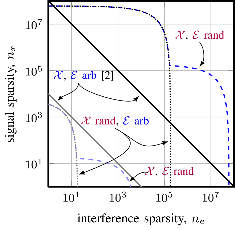
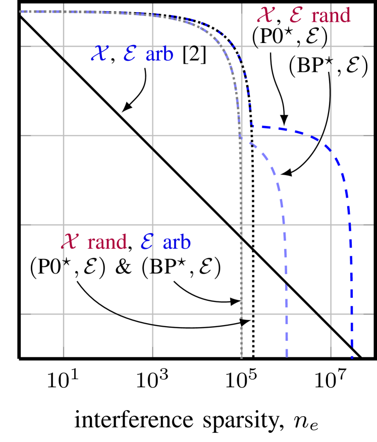
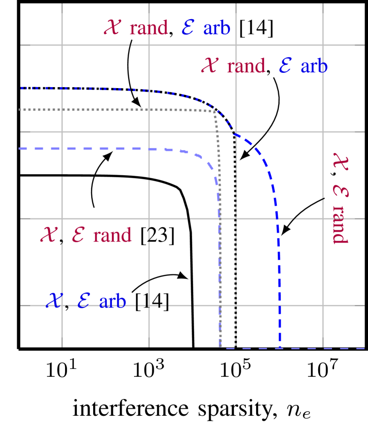
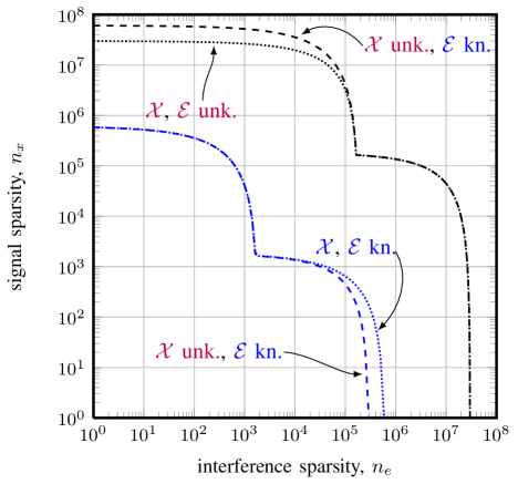
Figure 1: 𝐀𝐀\mathbf{A} and 𝐁𝐁\mathbf{B} are assumed to be unitary with m=na=nb=108𝑚subscript𝑛𝑎subscript𝑛𝑏superscript108m={n_{a}}={n_{b}}=10^{8} and μm=1/msubscript𝜇𝑚1𝑚\mu_{m}=1/\sqrt{m}. In (a) the darker curves in the upper-right are for m=108𝑚superscript108m=10^{8} and the lighter curves in the lower-left are for m=104𝑚superscript104m=10^{4}. In (c) we show the recovery regions only for (BP)superscriptBP(\textrm{BP}^{\star}). In each case, recovery is guaranteed with probability at least 11081superscript1081-10^{-8}.
\fref

fig:both_known shows the recovery conditions for the cases when both support sets 𝒳𝒳\mathcal{X} and \mathcal{E} are assumed to be known. For small problem dimensions, i.e., m=104𝑚superscript104m=10^{4}, the recovery conditions where both support sets are assumed to be arbitrary turn out to be less restrictive than for the case where both support sets are chosen at random. For large problem dimensions, i.e., m=108𝑚superscript108m=10^{8}, we see, however, that the probabilistic results of \frefthm:XkrEkr guarantee the recovery (with high probability) for larger nxsubscript𝑛𝑥n_{x} and nesubscript𝑛𝑒n_{e} than the deterministic results of [2] considering arbitrary support sets. Hence, the probabilistic recovery conditions presented here require a sufficiently large problem size in order to outperform the corresponding deterministic results. We furthermore see from \freffig:both_known that one can guarantee the recovery of signals having a larger number of non-zero entries if both support sets are chosen at random compared to the situation where 𝒳𝒳\mathcal{X} is random but \mathcal{E} is arbitrary.

IV-A2 Only \mathcal{E} known

\fref

fig:one_known shows the recovery conditions from Theorems 2 and 3 for the cases where only \mathcal{E} is known prior to recovery (the case of only 𝒳𝒳\mathcal{X} known behaves analogously). We see that for a random 𝒳𝒳\mathcal{X} and random \mathcal{E} successful recovery at high probability is guaranteed for significantly larger nxsubscript𝑛𝑥n_{x} and nesubscript𝑛𝑒n_{e} compared to the case where one or both support sets are assumed to be arbitrary. Hence, having more randomness in the support sets leads to less restrictive recovery guarantees. We now see that the recovery conditions for (P0,)superscriptP0(\textrm{P0}^{\star},\mathcal{E}) are slightly less restrictive than those for (BP,)superscriptBP(\textrm{BP}^{\star},\mathcal{E}).

IV-A3 No support-set knowledge

Finally, \freffig:none_known shows the recovery conditions for (BP)superscriptBP(\textrm{BP}^{\star}) for the case of no support-set knowledge. We see that for random 𝒳𝒳\mathcal{X} and \mathcal{E}, successful recovery is guaranteed for significantly larger nxsubscript𝑛𝑥n_{x} and nesubscript𝑛𝑒n_{e} compared to the case where one or both support sets are assumed to be arbitrary. As a comparison, we also show the recovery conditions derived in [14, Thm. 6] and the conditions from [23], the latter of which does not take into account the structure of the problem \frefeq:signal_model. We see that the recovery conditions derived in Theorems 5 and 6 are less restrictive, i.e., they guarantee the successful recovery (with high probability) for a larger number of nonzero coefficients in both the sparse signal vector 𝐱𝐱\mathbf{x} and the sparse interference 𝐞𝐞\mathbf{e}.

IV-A4 Non-unitary 𝐁𝐁\mathbf{B}

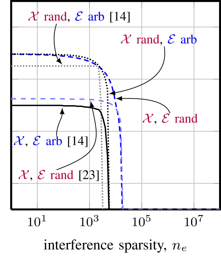
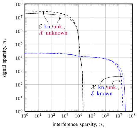
We now consider the setting where 𝐁𝐁\mathbf{B} is the concatenation of two unitary matrices and plot the corresponding recovery threshold for differing levels of support set knowledge in \freffig:3onb. For a fixed nxsubscript𝑛𝑥n_{x} and nasubscript𝑛𝑎{n_{a}}, we see that by increasing nbsubscript𝑛𝑏{n_{b}} and μbsubscript𝜇𝑏\mu_{b}, we suffer a significant loss in the number of non-zero entries of 𝐞𝐞\mathbf{e} that we can recover, when compared to the case where 𝐁𝐁\mathbf{B} is unitary. However, the number of non-zero entries of 𝐱𝐱\mathbf{x} that we can guarantee to recover is virtually unchanged—an effect which is also present in the deterministic recovery conditions [2].
Refer to caption
(a) 𝒳𝒳\mathcal{X} and \mathcal{E} known
Refer to caption
(b) \mathcal{E} known
Refer to caption
(c) 𝒳𝒳\mathcal{X} and \mathcal{E} unknown
Figure 2: 𝐀𝐀\mathbf{A} is assumed to be unitary and 𝐁𝐁\mathbf{B} is assumed to be the concatenation of two unitary matrices so that m=na=108𝑚subscript𝑛𝑎superscript108m={n_{a}}=10^{8}, nb=2nasubscript𝑛𝑏2subscript𝑛𝑎{n_{b}}=2{n_{a}}, μa=0subscript𝜇𝑎0\mu_{a}=0, and μb=μm=1/msubscript𝜇𝑏subscript𝜇𝑚1𝑚\mu_{b}=\mu_{m}=1/\sqrt{m} as described in [36, 37]. In (c) we show the recovery regions only for (BP)superscriptBP(\textrm{BP}^{\star}). In each case, recovery is guaranteed with probability at least 11081superscript1081-10^{-8}.

IV-B Impact of support-set knowledge

As detailed in [2], having knowledge of the support set of 𝐱𝐱\mathbf{x} or 𝐞𝐞\mathbf{e} implies that one can guarantee the recovery of 𝐱𝐱\mathbf{x} and 𝐞𝐞\mathbf{e} having up to twice as many non-zero entries (compared to the case of no support-set knowledge).

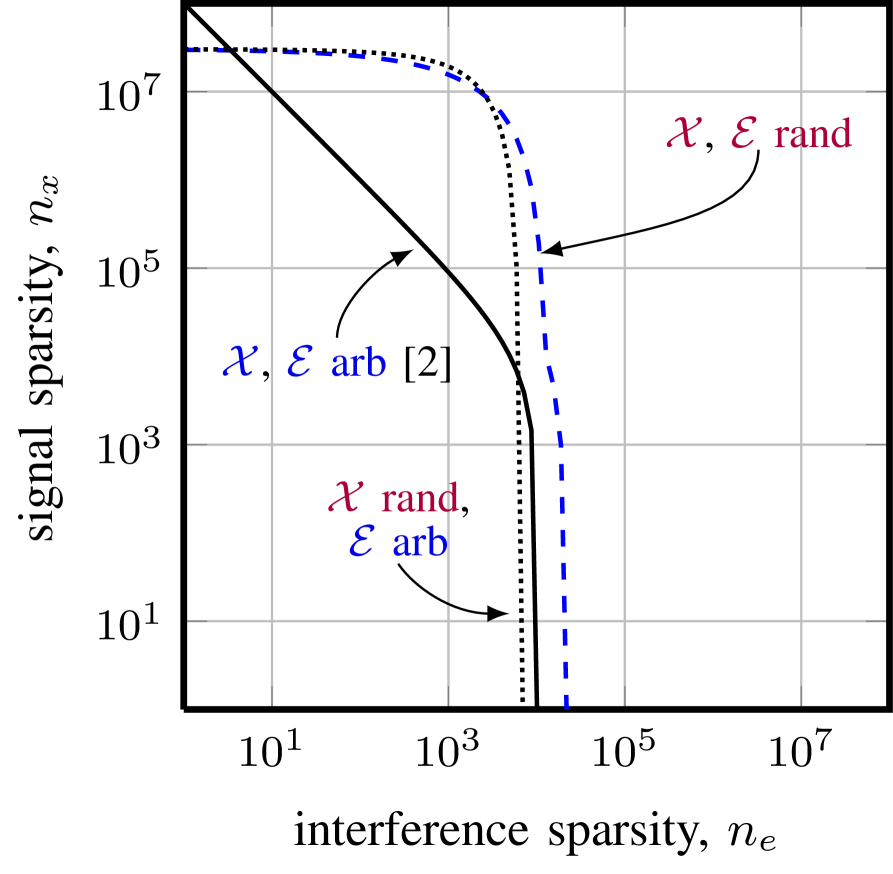
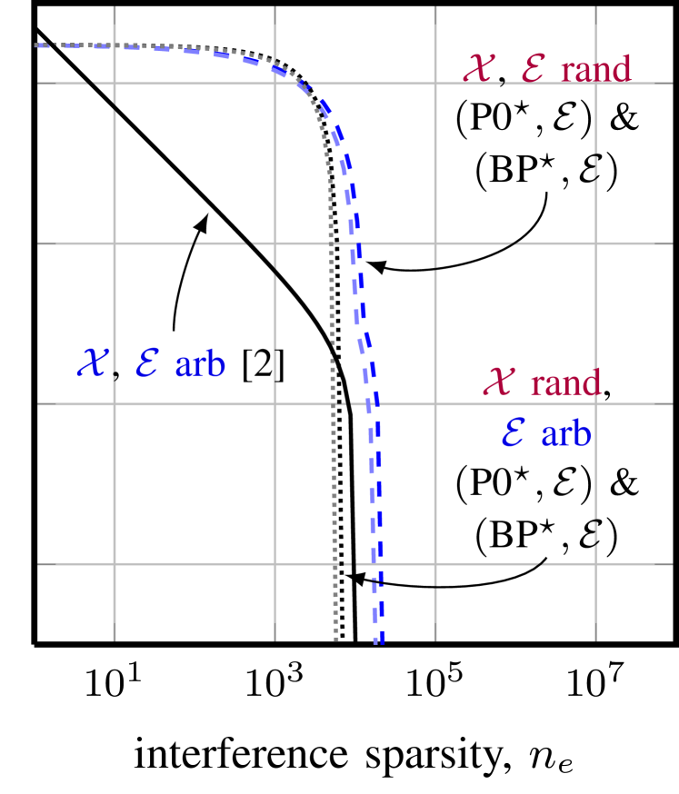
A similar behavior is also apparent in the probabilistic results presented here. Specifically, for unitary and maximally incoherent 𝐀𝐀\mathbf{A} and 𝐁𝐁\mathbf{B}, the recovery conditions in \freffig:knowledge using (2), (P0)P0(\textrm{P0}), and (P0,)superscriptP0(\textrm{P0}^{\star},\mathcal{E}) show a similar factor-of-two gain in the case where both 𝒳𝒳\mathcal{X} and \mathcal{E} are chosen at random. For example, knowledge of 𝒳𝒳\mathcal{X} enables one to recover a pair (𝐱,𝐞)𝐱𝐞(\mathbf{x},\mathbf{e}) with approximately twice as many non-zero entries compared to the case of not knowing 𝒳𝒳\mathcal{X}. In \freffig:knowledge_etf, we show the recovery conditions for the case where one dictionary is unitary, but the other is a concatenation of two unitary matrices, as described earlier in \frefsec:discussion. We again see that the extra support-set knowledge allows us to guarantee the recovery of a signal with more non-zero entries. It is interesting to note that in both of these scenarios, by adding the knowledge of one of the support sets, we increase the number of non-zero components we can guarantee to recover in the other signal component. For example, by knowing 𝒳𝒳\mathcal{X} prior to recovery, we can guarantee to recover a signal with more non-zero entries in 𝐞𝐞\mathbf{e}.

We note that a similar gain is apparent for 𝒳𝒳\mathcal{X} arbitrary and \mathcal{E} random, as well as for using (BP)BP(\textrm{BP}) and (BP,)superscriptBP(\textrm{BP}^{\star},\mathcal{E}) instead of (P0)P0(\textrm{P0}) and (P0,)superscriptP0(\textrm{P0}^{\star},\mathcal{E}).

Refer to caption
Figure 3: Impact of support-set knowledge on the recovery conditions for (2), (P0)P0(\textrm{P0}), and (P0,)superscriptP0(\textrm{P0}^{\star},\mathcal{E}) in the case where 𝒳𝒳\mathcal{X} and \mathcal{E} are both random. 𝐀𝐀\mathbf{A} and 𝐁𝐁\mathbf{B} are unitary with m=na=nb=106𝑚subscript𝑛𝑎subscript𝑛𝑏superscript106m={n_{a}}={n_{b}}=10^{6} (lower-left curves) and m=na=nb=108𝑚subscript𝑛𝑎subscript𝑛𝑏superscript108m={n_{a}}={n_{b}}=10^{8} (upper-right curves) and μm=1/msubscript𝜇𝑚1𝑚\mu_{m}=1/\sqrt{m}.
Refer to caption
Figure 4: Impact of support-set knowledge on the recovery conditions for (2), (P0)P0(\textrm{P0}), and (P0,)superscriptP0(\textrm{P0}^{\star},\mathcal{E}) in the case where 𝒳𝒳\mathcal{X} and \mathcal{E} are both random. In the top left we assume 𝐀𝐀\mathbf{A} is unitary and 𝐁𝐁\mathbf{B} is the concatenation of two unitary matrices so that m=na=108𝑚subscript𝑛𝑎superscript108m={n_{a}}=10^{8}, nb=2nasubscript𝑛𝑏2subscript𝑛𝑎{n_{b}}=2{n_{a}}, μa=0subscript𝜇𝑎0\mu_{a}=0, and μb=μm=1/msubscript𝜇𝑏subscript𝜇𝑚1𝑚\mu_{b}=\mu_{m}=1/\sqrt{m} as described in [36, 37]. For the curves in the bottom right (with 𝒳𝒳\mathcal{X} known/unknown and \mathcal{E} known) we reverse the roles of 𝐀𝐀\mathbf{A} and 𝐁𝐁\mathbf{B}, so that now 𝐁𝐁\mathbf{B} is unitary.

IV-C Asymptotic behavior of the recovery conditions

We now compare the asymptotic behavior of probabilistic and deterministic recovery conditions, i.e., we study the scaling behavior of nxsubscript𝑛𝑥n_{x} and nesubscript𝑛𝑒n_{e}. To this end, we are interested in the largest nxsubscript𝑛𝑥n_{x} for which recovery of 𝐱𝐱\mathbf{x} (and 𝐞𝐞\mathbf{e}) from 𝐳𝐳\mathbf{z} can be guaranteed with high probability. In particular, we consider the following models for the sparse interference vector 𝐞𝐞\mathbf{e}: i) Constant sparsity, i.e., ne=103subscript𝑛𝑒superscript103n_{e}=10^{3}, ii) sparsity proportional to the square root of the problem size, i.e., ne=msubscript𝑛𝑒𝑚n_{e}=\sqrt{m}, and iii) sparsity proportional to the problem size, i.e., ne=m/105subscript𝑛𝑒𝑚superscript105n_{e}=m/10^{5}.

\fref

fig:one_scaling shows the largest nxsubscript𝑛𝑥n_{x} for which recovery can be guaranteed using (BP,)superscriptBP(\textrm{BP}^{\star},\mathcal{E}). Here, \mathcal{E} is assumed to be known and arbitrary and 𝒳𝒳\mathcal{X} is unknown and chosen at random. Note that the other cases of support-set knowledge and arbitrary/random exhibit the same scaling behavior. We see from \freffig:one_scaling that for a constant interference sparsity (i.e., ne=103subscript𝑛𝑒superscript103n_{e}=10^{3}), the probabilistic and deterministic results show the same scaling behavior. For the cases where nesubscript𝑛𝑒n_{e} scales with m𝑚\sqrt{m} or m𝑚m, however, the deterministic thresholds developed in [2] result in worse scaling, while the behavior of the probabilistic guarantees derived in this paper remain unaffected.
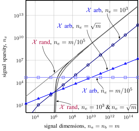
Refer to caption
Figure 5: Maximum signal sparsity nxsubscript𝑛𝑥n_{x} that ensures recovery of 𝐱𝐱\mathbf{x} for \mathcal{E} known and arbitrary. We assume ne=103subscript𝑛𝑒superscript103n_{e}=10^{3}, ne=msubscript𝑛𝑒𝑚n_{e}=\sqrt{m}, and ne=m/105subscript𝑛𝑒𝑚superscript105n_{e}=m/10^{5}. The probability of successful recovery is set to be at least 110151superscript10151-10^{-15}.

We now investigate the scaling behavior observed in \freffig:one_scaling analytically. Again, we only consider the case where 𝒳𝒳\mathcal{X} is unknown and chosen at random and \mathcal{E} is known and chosen arbitrarily; an analysis of the other cases yields similar results. Assume that 𝐀𝐀\mathbf{A} and 𝐁𝐁\mathbf{B} are unitary and maximally incoherent, i.e., μa=μb=0subscript𝜇𝑎subscript𝜇𝑏0\mu_{a}=\mu_{b}=0, na=nb=msubscript𝑛𝑎subscript𝑛𝑏𝑚{n_{a}}={n_{b}}=m, and μm=1/msubscript𝜇𝑚1𝑚\mu_{m}=1/\sqrt{m}. Then, by \frefthm:XurEka_BP, the recovery of 𝐱𝐱\mathbf{x} from 𝐳𝐳\mathbf{z} using (BP,)superscriptBP(\textrm{BP}^{\star},\mathcal{E}) is guaranteed with probability at least 13/na13subscript𝑛𝑎1-3/{n_{a}} (i.e., for β=log(na)𝛽subscript𝑛𝑎\beta=\log({n_{a}})) if

δe1/4nx/na+3μm2βne,𝛿superscript𝑒14subscript𝑛𝑥subscript𝑛𝑎3subscript𝜇𝑚2𝛽subscript𝑛𝑒\displaystyle\delta e^{-1/4}\geqslant\sqrt{n_{x}/{n_{a}}}+3\mu_{m}\sqrt{2\beta n_{e}},

and

2neμm2(log(na)+β)<(1δ)2,2subscript𝑛𝑒superscriptsubscript𝜇𝑚2subscript𝑛𝑎𝛽superscript1𝛿2\displaystyle 2n_{e}\mu_{m}^{2}(\log({n_{a}})+\beta)<(1-\delta)^{2},

hold. Combining these two conditions gives

e14m>nx+(32+2e14)nelog(m).superscript𝑒14𝑚subscript𝑛𝑥322superscript𝑒14subscript𝑛𝑒𝑚\displaystyle e^{-\frac{1}{4}}\sqrt{m}>\sqrt{n_{x}}+(3\sqrt{2}+2e^{-\frac{1}{4}})\sqrt{n_{e}\log(m)}. (16)

Hence, if nxmsimilar-tosubscript𝑛𝑥𝑚n_{x}\sim m and nem/log(m)similar-tosubscript𝑛𝑒𝑚𝑚n_{e}\sim m/\log(m), the condition \frefeq:examplecondition1 can be satisfied. Consequently, recovery of 𝐱𝐱\mathbf{x} (and of 𝐞𝐞\mathbf{e}) is guaranteed with probability at least 13/m13𝑚1-3/m even if nxsubscript𝑛𝑥n_{x} scales linearly in the number of (corrupted) measurements m𝑚m and nesubscript𝑛𝑒n_{e} scales near-linearly (i.e., with m/log(m)𝑚𝑚m/\log(m)) in m𝑚m.

We finally note that the recovery guarantees in [16] also allow for the sparsity of the interference vector to scale near-linearly in the number of measurements. The results in [16], however, require the matrix 𝐀𝐀\mathbf{A} to be random and 𝐁𝐁\mathbf{B} to be orthogonal, whereas the recovery guarantees shown here are for arbitrary pairs of dictionaries 𝐀𝐀\mathbf{A} and 𝐁𝐁\mathbf{B} (characterized by the coherence parameters) and for varying degrees of support-set knowledge.

IV-D No error component

It is worth briefly discussing how our results behave when there is no error, that is when ne=0subscript𝑛𝑒0n_{e}=0. In this case, the relevant setting is with 𝒳𝒳\mathcal{X} unknown and chosen uniformly at random. As \frefthm:XurEka_P0 holds for any 𝐁𝐁\mathbf{B}, it suffices to take 𝐁𝐁\mathbf{B} equal to a single column888Taking 𝐁𝐁\mathbf{B} to be the zero-matrix and so removing all the terms that appear in the recovery conditions also leads to the same scaling behavior., since ne=0subscript𝑛𝑒0n_{e}=0 means we do not consider any component of 𝐁𝐁\mathbf{B} when attempting to recover the signals. And since the mutual coherence μmsubscript𝜇𝑚\mu_{m} only appears as a product with nesubscript𝑛𝑒n_{e}, it does not matter what we assume μmsubscript𝜇𝑚\mu_{m} to be. Thus by taking ne=0subscript𝑛𝑒0n_{e}=0 and applying \frefthm:XurEka_P0 we find that for (P0,)superscriptP0(\textrm{P0}^{\star},\mathcal{E}), recovery is guaranteed with probability at least 1eβ1superscript𝑒𝛽1-e^{-\beta} if

e14(1nxμa2)\norml2𝐀nxna+12μaβnx.superscript𝑒141subscript𝑛𝑥superscriptsubscript𝜇𝑎2\norm𝑙2𝐀subscript𝑛𝑥subscript𝑛𝑎12subscript𝜇𝑎𝛽subscript𝑛𝑥\displaystyle e^{-\frac{1}{4}}(1-n_{x}\mu_{a}^{2})\geqslant\norm{l2}{\mathbf{A}}\sqrt{\frac{n_{x}}{{n_{a}}}}+12\mu_{a}\sqrt{\beta n_{x}}. (17)

For (BP,)superscriptBP(\textrm{BP}^{\star},\mathcal{E}), recovery is guaranteed with probability at least 13eβ13superscript𝑒𝛽1-3e^{-\beta} if

e14(12nxμa2(log(na)+β))\norml2𝐀nxna+12μaβnx.superscript𝑒1412subscript𝑛𝑥superscriptsubscript𝜇𝑎2subscript𝑛𝑎𝛽\norm𝑙2𝐀subscript𝑛𝑥subscript𝑛𝑎12subscript𝜇𝑎𝛽subscript𝑛𝑥\displaystyle e^{-\frac{1}{4}}\mathopen{}\left(1-\sqrt{2n_{x}\mu_{a}^{2}(\log({n_{a}})+\beta)}\right)\geqslant\norm{l2}{\mathbf{A}}\sqrt{\frac{n_{x}}{{n_{a}}}}+12\mu_{a}\sqrt{\beta n_{x}}. (18)

Now assume that μa1/msimilar-tosubscript𝜇𝑎1𝑚\mu_{a}\sim 1/\sqrt{m}, \norml2𝐀2=na/m\norm𝑙2superscript𝐀2subscript𝑛𝑎𝑚\norm{l2}{\mathbf{A}}^{2}={n_{a}}/m, and that β=log(na)𝛽subscript𝑛𝑎\beta=\log({n_{a}}). Then (after ignoring lower order terms), we find that (17) and (18) imply recovery with probability at least 11/na11subscript𝑛𝑎1-1/{n_{a}} and 13/na13subscript𝑛𝑎1-3/{n_{a}}, respectively, provided that

mCnxlog(na),𝑚Csubscript𝑛𝑥subscript𝑛𝑎\displaystyle m\geqslant\mathrm{C}\,n_{x}\log({n_{a}}),

for some positive constant CC\mathrm{C}. This result is in accordance with [23], the RIP-based proof of [38] which requires mC0nxlog(na/nx)𝑚subscriptC0subscript𝑛𝑥subscript𝑛𝑎subscript𝑛𝑥m\geqslant\mathrm{C}_{0}\,n_{x}\log({n_{a}}/n_{x}) to guarantee recovery with high probability, and the random sub-sampling model of [27], which, for a maximally incoherent sparsity basis and measurement matrix999For example, measuring with a randomly sub-sampled Fourier matrix and taking the Identity matrix as the sparsity basis, so that with the differently normalized definition of coherence as in [27], μa=1subscript𝜇𝑎1\mu_{a}=1., requires mC1nxlog(na)𝑚subscriptC1subscript𝑛𝑥subscript𝑛𝑎m\geqslant\mathrm{C}_{1}\,n_{x}\log({n_{a}}) to guarantee recovery with high probability. Thus, our results reduce to some of the existing results in the setting where there is no error.

V Conclusions

In this paper, we have presented novel coherence-based recovery guarantees for sparsely corrupted signals in the probabilistic setting. In particular, we have studied the case where the sparse signal and/or sparse interference vectors are modeled as random and the dictionaries 𝐀𝐀\mathbf{A} and 𝐁𝐁\mathbf{B} are solely characterized by their coherence parameters. Our recovery guarantees complete all missing cases of support-set knowledge and improve and refine the results in [2, 14]. Furthermore, we have shown that the reconstruction of sparse signals is guaranteed with high probability, even if the number of non-zero entries in both the sparse signal and sparse interference are allowed to scale (near) linearly with the number of (corrupted) measurements.

There are many avenues for follow-on work. The derivation of probabilistic recovery guarantees for the more general setting studied in [13], i.e., 𝐳=𝐀𝐱+𝐁𝐞+𝐧𝐳𝐀𝐱𝐁𝐞𝐧\mathbf{z}=\mathbf{A}\mathbf{x}+\mathbf{B}\mathbf{e}+\mathbf{n} with 𝐧𝐧\mathbf{n} being additive noise and 𝐱𝐱\mathbf{x} and 𝐞𝐞\mathbf{e} being approximately sparse (rather than perfectly sparse), is left for future work. In addition, our framework could be generalized to the setting where we split both the known and the unknown support sets into a random and arbitrary part, resulting in four parts, as outlined in \frefsec:rin. Finally, the derivation of probabilistic uncertainty relations for pairs of general dictionaries is an interesting open problem and would complete the deterministic uncertainty relations in [14, 2].

Acknowledgments

The authors would like to thank C. Aubel, R. G. Baraniuk, H. Bölcskei, I. Koch, P. Kuppinger, A. Pope, and E. Riegler for inspiring discussions. We would also like to thank the anonymous reviewers for their valuable comments, which improved the overall quality of the paper.

Appendix A Bounds on σmin(𝐃𝒳,)subscript𝜎subscript𝐃𝒳\sigma_{\min}(\mathbf{D}_{\mathcal{X},\mathcal{E}})

We now derive probabilistic bounds on σmin(𝐃𝒳,)subscript𝜎subscript𝐃𝒳\sigma_{\min}(\mathbf{D}_{\mathcal{X},\mathcal{E}}), which are key in showing when the recovery from sparsely corrupted signals succeeds. We extend [14, Lemma 7] to the case where both supports 𝒳𝒳\mathcal{X} and \mathcal{E} are chosen at random and give improved results for the case where only one support set is random. First, we require the following two results from [23].

Theorem 7 (Thm. 8 of [23])

Let 𝐌m×n𝐌superscript𝑚𝑛\mathbf{M}\in\mathbb{C}^{m\times n} be a matrix. Let 𝒮{1,2,,n}𝒮12𝑛\mathcal{S}\subseteq\{1,2,\ldots,n\} be a set of size s𝑠s drawn uniformly at random. Fix q1𝑞1q\geqslant 1, then for each pmax{2,2log(rank(𝐌𝐑𝒮)),q/2}𝑝22ranksubscript𝐌𝐑𝒮𝑞2p\geqslant\max\{2,2\log(\operatorname{rank}(\mathbf{M}\mathbf{R}_{\mathcal{S}})),q/2\} we have

𝔼q[\norml2l2𝐌𝐑𝒮]3p\norml1l2𝐌+sn\norml2l2𝐌,superscript𝔼𝑞delimited-[]\norm𝑙2𝑙2subscript𝐌𝐑𝒮3𝑝\norm𝑙1𝑙2𝐌𝑠𝑛\norm𝑙2𝑙2𝐌\displaystyle\mathbb{E}^{q}\mathopen{}\left[\norm{l2l2}{\mathbf{M}\mathbf{R}_{\mathcal{S}}}\right]\leqslant 3\sqrt{p}\norm{l1l2}{\mathbf{M}}+\sqrt{\frac{s}{n}}\norm{l2l2}{\mathbf{M}},

where \norml1l2𝐌=sup𝐯n\norml2𝐌𝐯/\norml1𝐯\norm𝑙1𝑙2𝐌subscriptsupremum𝐯superscript𝑛\norm𝑙2𝐌𝐯\norm𝑙1𝐯\norm{l1l2}{\mathbf{M}}=\sup_{\mathbf{v}\in\mathbb{C}^{n}}\norm{l2}{\mathbf{M}\mathbf{v}}/\norm{l1}{\mathbf{v}} and is the maximum 2subscript2\ell_{2}-norm of the columns of 𝐌𝐌\mathbf{M}.

Lemma 8 (Eq. 6.1 of [23])

Let 𝐌m×n𝐌superscript𝑚𝑛\mathbf{M}\in\mathbb{C}^{m\times n} be a matrix with coherence μ𝜇\mu and let 𝒮{1,2,,n}𝒮12𝑛\mathcal{S}\subseteq\{1,2,\ldots,n\} be a set of size s𝑠s chosen uniformly at random. Then, for βlog(s)𝛽𝑠\beta\geqslant\log(s) and q=4β𝑞4𝛽q=4\beta

𝔼q[\norml2l2𝐌𝒮H𝐌𝒮𝐈]12μβs+𝟙[μ0]2sn\norml2l2𝐌2.superscript𝔼𝑞delimited-[]\norm𝑙2𝑙2superscriptsubscript𝐌𝒮𝐻subscript𝐌𝒮𝐈12𝜇𝛽𝑠1delimited-[]𝜇02𝑠𝑛\norm𝑙2𝑙2superscript𝐌2\displaystyle\mathbb{E}^{q}\mathopen{}\left[\norm{l2l2}{\mathbf{M}_{\mathcal{S}}^{H}\mathbf{M}_{\mathcal{S}}-\mathbf{I}}\right]\leqslant 12\mu\sqrt{\beta s}+\mathbbm{1}[{\mu\neq 0}]\frac{2s}{n}\norm{l2l2}{\mathbf{M}}^{2}.

Note that the result in [23, Eq. 6.1] does not include the indicator function 𝟙[μ0]1delimited-[]𝜇0\mathbbm{1}[{\mu\neq 0}]. It is, however, straightforward to verify that if 𝐌𝐌\mathbf{M} is orthonormal, then μ=0𝜇0\mu=0 and hence, \norml2l2𝐌𝒮H𝐌𝒮𝐈=0\norm𝑙2𝑙2superscriptsubscript𝐌𝒮𝐻subscript𝐌𝒮𝐈0\norm{l2l2}{\mathbf{M}_{\mathcal{S}}^{H}\mathbf{M}_{\mathcal{S}}-\mathbf{I}}=0 for all sets 𝒮𝒮\mathcal{S}.

We now state the main result for σmin(𝐃𝒳,)subscript𝜎subscript𝐃𝒳\sigma_{\min}(\mathbf{D}_{\mathcal{X},\mathcal{E}}).

Theorem 9

Choose βlog(nx)𝛽subscript𝑛𝑥\beta\geqslant\log(n_{x}), q=4β𝑞4𝛽q=4\beta and assume that 𝐀𝐀\mathbf{A} and 𝐁𝐁\mathbf{B} are characterized by the coherence parameters μasubscript𝜇𝑎\mu_{a}, μbsubscript𝜇𝑏\mu_{b}, and μmsubscript𝜇𝑚\mu_{m}. If i) 𝒳𝒳\mathcal{X}is chosen uniformly at random with cardinality nxsubscript𝑛𝑥n_{x}, \mathcal{E} is arbitrary, and (3) holds, or ii) \mathcal{E}is chosen uniformly at random with cardinality nesubscript𝑛𝑒n_{e}, 𝒳𝒳\mathcal{X} is arbitrary, and (13) holds, or iii) both 𝒳𝒳\mathcal{X} and \mathcal{E} are chosen uniformly at random with cardinalities nxsubscript𝑛𝑥n_{x} and nesubscript𝑛𝑒n_{e} respectively, and (4) holds, then

{\norml2l2𝐃𝒳,H𝐃𝒳,𝐈δ}eβ,\norm𝑙2𝑙2superscriptsubscript𝐃𝒳𝐻subscript𝐃𝒳𝐈𝛿superscript𝑒𝛽\displaystyle\mathbb{P}\mathopen{}\left\{\norm{l2l2}{\mathbf{D}_{\mathcal{X},\mathcal{E}}^{H}\mathbf{D}_{\mathcal{X},\mathcal{E}}-\mathbf{I}}\geqslant\delta\right\}\leqslant e^{-\beta}, (19)

and if (3), (4) or (13) hold with δ=1𝛿1\delta=1, then

{σmin(𝐃𝒳,)=0}eβ.subscript𝜎subscript𝐃𝒳0superscript𝑒𝛽\displaystyle\mathbb{P}\mathopen{}\left\{\sigma_{\min}(\mathbf{D}_{\mathcal{X},\mathcal{E}})=0\right\}\leqslant e^{-\beta}. (20)
Proof:

The proof follows that of [14, Lemma 7]. We start by defining the hollow Gram matrix

𝐇=𝐃𝒳,H𝐃𝒳,𝐈=[𝐀𝒳H𝐀𝒳𝐈𝐀𝒳H𝐁𝐁H𝐀𝒳𝐁H𝐁𝐈].𝐇superscriptsubscript𝐃𝒳𝐻subscript𝐃𝒳𝐈matrixsubscriptsuperscript𝐀𝐻𝒳subscript𝐀𝒳𝐈superscriptsubscript𝐀𝒳𝐻subscript𝐁subscriptsuperscript𝐁𝐻subscript𝐀𝒳subscriptsuperscript𝐁𝐻subscript𝐁𝐈\displaystyle\mathbf{H}=\mathbf{D}_{\mathcal{X},\mathcal{E}}^{H}\mathbf{D}_{\mathcal{X},\mathcal{E}}-\mathbf{I}=\begin{bmatrix}\mathbf{A}^{H}_{\mathcal{X}}\mathbf{A}_{\mathcal{X}}-\mathbf{I}&\mathbf{A}_{\mathcal{X}}^{H}\mathbf{B}_{\mathcal{E}}\\ \mathbf{B}^{H}_{\mathcal{E}}\mathbf{A}_{\mathcal{X}}&\mathbf{B}^{H}_{\mathcal{E}}\mathbf{B}_{\mathcal{E}}-\mathbf{I}\end{bmatrix}.

Splitting 𝐇𝐇\mathbf{H} into diagonal and off-diagonal blocks and applying the triangle inequality leads to

\norml2l2𝐇\norm𝑙2𝑙2𝐇\displaystyle\norm{l2l2}{\mathbf{H}} \norml2l2[𝐀𝒳H𝐀𝒳𝐈00𝐁H𝐁𝐈]+\norml2l2[0𝐀𝒳H𝐁𝐁H𝐀𝒳0]absent\norm𝑙2𝑙2matrixsubscriptsuperscript𝐀𝐻𝒳subscript𝐀𝒳𝐈00subscriptsuperscript𝐁𝐻subscript𝐁𝐈\norm𝑙2𝑙2matrix0superscriptsubscript𝐀𝒳𝐻subscript𝐁subscriptsuperscript𝐁𝐻subscript𝐀𝒳0\displaystyle\leqslant\norm{l2l2}{\begin{bmatrix}\mathbf{A}^{H}_{\mathcal{X}}\mathbf{A}_{\mathcal{X}}-\mathbf{I}&0\\ 0&\mathbf{B}^{H}_{\mathcal{E}}\mathbf{B}_{\mathcal{E}}-\mathbf{I}\end{bmatrix}}\!\!\!\!\!\!+\norm{l2l2}{\begin{bmatrix}0&\mathbf{A}_{\mathcal{X}}^{H}\mathbf{B}_{\mathcal{E}}\\ \mathbf{B}^{H}_{\mathcal{E}}\mathbf{A}_{\mathcal{X}}&0\end{bmatrix}}
max{\norml2l2𝐀𝒳H𝐀𝒳𝐈,\norml2l2𝐁H𝐁𝐈}+\norml2l2𝐁H𝐀𝒳absent\norm𝑙2𝑙2subscriptsuperscript𝐀𝐻𝒳subscript𝐀𝒳𝐈\norm𝑙2𝑙2subscriptsuperscript𝐁𝐻subscript𝐁𝐈\norm𝑙2𝑙2subscriptsuperscript𝐁𝐻subscript𝐀𝒳\displaystyle\leqslant\max\mathopen{}\left\{\norm{l2l2}{\mathbf{A}^{H}_{\mathcal{X}}\mathbf{A}_{\mathcal{X}}-\mathbf{I}},\norm{l2l2}{\mathbf{B}^{H}_{\mathcal{E}}\mathbf{B}_{\mathcal{E}}-\mathbf{I}}\right\}+\norm{l2l2}{\mathbf{B}^{H}_{\mathcal{E}}\mathbf{A}_{\mathcal{X}}}
\norml2l2𝐀𝒳H𝐀𝒳𝐈+\norml2l2𝐁H𝐁𝐈+\norml2l2𝐁H𝐀𝒳.absent\norm𝑙2𝑙2subscriptsuperscript𝐀𝐻𝒳subscript𝐀𝒳𝐈\norm𝑙2𝑙2subscriptsuperscript𝐁𝐻subscript𝐁𝐈\norm𝑙2𝑙2subscriptsuperscript𝐁𝐻subscript𝐀𝒳\displaystyle\leqslant\norm{l2l2}{\mathbf{A}^{H}_{\mathcal{X}}\mathbf{A}_{\mathcal{X}}-\mathbf{I}}+\norm{l2l2}{\mathbf{B}^{H}_{\mathcal{E}}\mathbf{B}_{\mathcal{E}}-\mathbf{I}}+\norm{l2l2}{\mathbf{B}^{H}_{\mathcal{E}}\mathbf{A}_{\mathcal{X}}}.

Since the q𝑞qth moment effectively defines an qsubscript𝑞\ell_{q}-norm, it satisfies the triangle inequality, namely, 𝔼q[|X+Y|]𝔼q[|X|]+𝔼q[|Y|]superscript𝔼𝑞delimited-[]𝑋𝑌superscript𝔼𝑞delimited-[]𝑋superscript𝔼𝑞delimited-[]𝑌\mathbb{E}^{q}\mathopen{}\left[\mathopen{}\left\lvert X+Y\right\rvert\right]\leqslant\mathbb{E}^{q}\mathopen{}\left[\mathopen{}\left\lvert X\right\rvert\right]+\mathbb{E}^{q}\mathopen{}\left[\mathopen{}\left\lvert Y\right\rvert\right]. Hence, it follows that

𝔼q[\norml2l2𝐇]superscript𝔼𝑞delimited-[]\norm𝑙2𝑙2𝐇absent\displaystyle\mathbb{E}^{q}\mathopen{}\left[\norm{l2l2}{\mathbf{H}}\right]\leqslant 𝔼q[\norml2l2𝐀𝒳H𝐀𝒳𝐈]+𝔼q[\norml2l2𝐁H𝐁𝐈]+𝔼q[\norml2l2𝐁H𝐀𝒳].superscript𝔼𝑞delimited-[]\norm𝑙2𝑙2subscriptsuperscript𝐀𝐻𝒳subscript𝐀𝒳𝐈superscript𝔼𝑞delimited-[]\norm𝑙2𝑙2subscriptsuperscript𝐁𝐻subscript𝐁𝐈superscript𝔼𝑞delimited-[]\norm𝑙2𝑙2subscriptsuperscript𝐁𝐻subscript𝐀𝒳\displaystyle\ \mathbb{E}^{q}\mathopen{}\left[\norm{l2l2}{\mathbf{A}^{H}_{\mathcal{X}}\mathbf{A}_{\mathcal{X}}-\mathbf{I}}\right]+\mathbb{E}^{q}\mathopen{}\left[\norm{l2l2}{\mathbf{B}^{H}_{\mathcal{E}}\mathbf{B}_{\mathcal{E}}-\mathbf{I}}\right]+\mathbb{E}^{q}\mathopen{}\left[\norm{l2l2}{\mathbf{B}^{H}_{\mathcal{E}}\mathbf{A}_{\mathcal{X}}}\right]. (21)

We now separately bound each of the terms in (21) and we do this for each case where 𝒳𝒳\mathcal{X} and \mathcal{E} is either chosen at random or arbitrarily. If 𝒳𝒳\mathcal{X} is chosen uniformly at random, then it follows from \freflem:momentbound that

𝔼q[\norml2l2𝐀𝒳H𝐀𝒳𝐈]12μaβnx+𝟙[μa0]2nxna\norml2l2𝐀,superscript𝔼𝑞delimited-[]\norm𝑙2𝑙2subscriptsuperscript𝐀𝐻𝒳subscript𝐀𝒳𝐈12subscript𝜇𝑎𝛽subscript𝑛𝑥1delimited-[]subscript𝜇𝑎02subscript𝑛𝑥subscript𝑛𝑎\norm𝑙2𝑙2𝐀\displaystyle\mathbb{E}^{q}\mathopen{}\left[\norm{l2l2}{\mathbf{A}^{H}_{\mathcal{X}}\mathbf{A}_{\mathcal{X}}-\mathbf{I}}\right]\leqslant 12\mu_{a}\sqrt{\beta n_{x}}+\mathbbm{1}[{\mu_{a}\neq 0}]\frac{2n_{x}}{{n_{a}}}\norm{l2l2}{\mathbf{A}}, (22)

for any 4β=q4log(nx)4𝛽𝑞4subscript𝑛𝑥4\beta=q\geqslant 4\log(n_{x}). If 𝒳𝒳\mathcal{X} is allowed to be arbitrary, then for all 𝒳𝒳\mathcal{X} we have

\norml2l2𝐀𝒳H𝐀𝒳𝐈maxkjk|[𝐀𝒳H𝐀𝒳]j,k|(nx1)μa,\norm𝑙2𝑙2subscriptsuperscript𝐀𝐻𝒳subscript𝐀𝒳𝐈subscript𝑘subscript𝑗𝑘subscriptdelimited-[]superscriptsubscript𝐀𝒳𝐻subscript𝐀𝒳𝑗𝑘subscript𝑛𝑥1subscript𝜇𝑎\displaystyle\norm{l2l2}{\mathbf{A}^{H}_{\mathcal{X}}\mathbf{A}_{\mathcal{X}}-\mathbf{I}}\leqslant\max_{k}\sum_{j\neq k}\mathopen{}\left\lvert[\mathbf{A}_{\mathcal{X}}^{H}\mathbf{A}_{\mathcal{X}}]_{j,k}\right\rvert\leqslant(n_{x}-1)\mu_{a}, (23)

where the first inequality follows from the Geršgorin disc theorem [39, Thm. 6.1.1] and the second inequality is a consequence of the definition of μasubscript𝜇𝑎\mu_{a}. By reversing the role of 𝐀𝐀\mathbf{A} and 𝐁𝐁\mathbf{B}, we get the analogous bounds for the right-hand side (RHS) term 𝔼q[\norml2l2𝐁H𝐁𝐈]superscript𝔼𝑞delimited-[]\norm𝑙2𝑙2subscriptsuperscript𝐁𝐻subscript𝐁𝐈\mathbb{E}^{q}\mathopen{}\left[\norm{l2l2}{\mathbf{B}^{H}_{\mathcal{E}}\mathbf{B}_{\mathcal{E}}-\mathbf{I}}\right] in \frefeq:one_3terms.

For the third summand appearing in the RHS of (21), let us first consider the case where \mathcal{E} is chosen arbitrarily and 𝒳𝒳\mathcal{X} uniformly at random. We then want to apply \frefthm:211 to 𝐌=𝐁H𝐀𝐌superscriptsubscript𝐁𝐻𝐀\mathbf{M}=\mathbf{B}_{\mathcal{E}}^{H}\mathbf{A} and 𝐑𝒳subscript𝐑𝒳\mathbf{R}_{\mathcal{X}}. Since 𝐌𝐑𝒳subscript𝐌𝐑𝒳\mathbf{M}\mathbf{R}_{\mathcal{X}} has nesubscript𝑛𝑒n_{e} rows and nxsubscript𝑛𝑥n_{x} non-zero columns, rank(𝐌𝐑𝒳)min{nx,ne}ranksubscript𝐌𝐑𝒳subscript𝑛𝑥subscript𝑛𝑒\operatorname{rank}(\mathbf{M}\mathbf{R}_{\mathcal{X}})\leqslant\min\{n_{x},n_{e}\} and thus we can apply \frefthm:211 with q=2p=4β𝑞2𝑝4𝛽q=2p=4\beta where q4min{log(nx),log(ne)}4log(rank(𝐌𝐑𝒳))𝑞4subscript𝑛𝑥subscript𝑛𝑒4ranksubscript𝐌𝐑𝒳q\geqslant 4\min\{\log(n_{x}),\log(n_{e})\}\geqslant 4\log(\operatorname{rank}(\mathbf{M}\mathbf{R}_{\mathcal{X}})) to get

𝔼q[\norml2l2𝐁H𝐀𝒳]superscript𝔼𝑞delimited-[]\norm𝑙2𝑙2subscriptsuperscript𝐁𝐻subscript𝐀𝒳\displaystyle\mathbb{E}^{q}\mathopen{}\left[\norm{l2l2}{\mathbf{B}^{H}_{\mathcal{E}}\mathbf{A}_{\mathcal{X}}}\right] =𝔼𝒳q[\norml2l2𝐁H𝐀𝒳]absentsubscriptsuperscript𝔼𝑞𝒳delimited-[]\norm𝑙2𝑙2subscriptsuperscript𝐁𝐻subscript𝐀𝒳\displaystyle=\mathbb{E}^{q}_{\mathcal{X}}\mathopen{}\left[\norm{l2l2}{\mathbf{B}^{H}_{\mathcal{E}}\mathbf{A}_{\mathcal{X}}}\right] (24a)
3p\norml1l2𝐁H𝐀+nxna\norml2l2𝐁H𝐀absent3𝑝\norm𝑙1𝑙2subscriptsuperscript𝐁𝐻𝐀subscript𝑛𝑥subscript𝑛𝑎\norm𝑙2𝑙2superscriptsubscript𝐁𝐻𝐀\displaystyle\leqslant 3\sqrt{p}\norm{l1l2}{\mathbf{B}^{H}_{\mathcal{E}}\mathbf{A}}+\sqrt{\frac{n_{x}}{{n_{a}}}}\norm{l2l2}{\mathbf{B}_{\mathcal{E}}^{H}\mathbf{A}}
3μm2βne+nxna\norml2l2𝐁H𝐀,absent3subscript𝜇𝑚2𝛽subscript𝑛𝑒subscript𝑛𝑥subscript𝑛𝑎\norm𝑙2𝑙2superscript𝐁𝐻𝐀\displaystyle\leqslant 3\mu_{m}\sqrt{2\beta n_{e}}+\sqrt{\frac{n_{x}}{{n_{a}}}}\norm{l2l2}{\mathbf{B}^{H}\mathbf{A}}, (24b)

where the entries of 𝐁H𝐀subscriptsuperscript𝐁𝐻𝐀\mathbf{B}^{H}_{\mathcal{E}}\mathbf{A} are bounded by the mutual coherence μmsubscript𝜇𝑚\mu_{m}. The case where \mathcal{E} is random and 𝒳𝒳\mathcal{X} is arbitrary follows by reversing the roles of 𝐀𝐀\mathbf{A} and 𝐁𝐁\mathbf{B}.

Now consider the case where both \mathcal{E} and 𝒳𝒳\mathcal{X} are random. We can set 𝐌=𝐁H𝐀𝐌superscript𝐁𝐻𝐀\mathbf{M}=\mathbf{B}^{H}\mathbf{A} so that we may write 𝔼q[\norml2l2𝐁H𝐀𝒳]=𝔼q[𝔼𝒳q[\norml2l2𝐑𝐌𝐑𝒳]]superscript𝔼𝑞delimited-[]\norm𝑙2𝑙2subscriptsuperscript𝐁𝐻subscript𝐀𝒳subscriptsuperscript𝔼𝑞delimited-[]subscriptsuperscript𝔼𝑞𝒳delimited-[]\norm𝑙2𝑙2subscript𝐑subscript𝐌𝐑𝒳\mathbb{E}^{q}\mathopen{}\left[\norm{l2l2}{\mathbf{B}^{H}_{\mathcal{E}}\mathbf{A}_{\mathcal{X}}}\right]=\mathbb{E}^{q}_{\mathcal{E}}\mathopen{}\left[\mathbb{E}^{q}_{\mathcal{X}}\mathopen{}\left[\norm{l2l2}{\mathbf{R}_{\mathcal{E}}\mathbf{M}\mathbf{R}_{\mathcal{X}}}\right]\right] in order to apply \frefthm:211 to first bound the inner expectation, and then to bound the resulting outer expectation. However, this approach results in a worse bound compared to reusing (24b), which does not depend on \mathcal{E} and hence holds for all \mathcal{E}. By also taking the expectation in (24a) with respect to \mathcal{E} instead of 𝒳𝒳\mathcal{X} and bounding similarly, we get that

𝔼q[\norml2l2𝐁H𝐀𝒳]superscript𝔼𝑞delimited-[]\norm𝑙2𝑙2subscriptsuperscript𝐁𝐻subscript𝐀𝒳absent\displaystyle\mathbb{E}^{q}\mathopen{}\left[\norm{l2l2}{\mathbf{B}^{H}_{\mathcal{E}}\mathbf{A}_{\mathcal{X}}}\right]\leqslant min{3μm2βnx+nenb\norml2l2𝐀H𝐁,\displaystyle\,\min\left\{3\mu_{m}\sqrt{2\beta n_{x}}+\sqrt{\frac{n_{e}}{{n_{b}}}}\norm{l2l2}{\mathbf{A}^{H}\mathbf{B}},\right.
3μm2βne+nxna\norml2l2𝐀H𝐁},\displaystyle\ \,\qquad\left.3\mu_{m}\sqrt{2\beta n_{e}}+\sqrt{\frac{n_{x}}{{n_{a}}}}\norm{l2l2}{\mathbf{A}^{H}\mathbf{B}}\right\}, (25)

for any βmin{log(nx),log(ne)}𝛽subscript𝑛𝑥subscript𝑛𝑒\beta\geqslant\min\{\log(n_{x}),\log(n_{e})\}. Combining (22), (23), (24b), and (25) with the analogous results for 𝐁𝐁\mathbf{B} and \mathcal{E} leads to the conditions (3), (4), and (13).

Due to (22) and the analogous result for 𝐁subscript𝐁\mathbf{B}_{\mathcal{E}}, if 𝒳𝒳\mathcal{X} is chosen at random, we require βlog(nx)𝛽subscript𝑛𝑥\beta\geqslant\log(n_{x}), if \mathcal{E} is chosen at random we need βlog(ne)𝛽subscript𝑛𝑒\beta\geqslant\log(n_{e}), and if both 𝒳𝒳\mathcal{X} and \mathcal{E} are chosen at random, both of these conditions need to be satisfied, namely that βmax{log(nx),log(ne)}𝛽subscript𝑛𝑥subscript𝑛𝑒\beta\geqslant\max\{\log(n_{x}),\log(n_{e})\}.

We now show that the conditions (3), (4), and (13) are sufficient to show that (19) holds. Chebyshev’s Inequality [40, Sec. 1.3] states that for a random variable X𝑋X and a function f:+:𝑓superscriptf\colon\mathbb{R}\rightarrow\mathbb{R}^{+}

{X𝒜}𝔼[f(X)]inf{f(x):x𝒜}.𝑋𝒜𝔼delimited-[]𝑓𝑋infimumconditional-set𝑓𝑥𝑥𝒜\displaystyle\mathbb{P}\mathopen{}\left\{X\in\mathcal{A}\right\}\leqslant\frac{\mathbb{E}\mathopen{}\left[f(X)\right]}{\inf\mathopen{}\left\{f(x)\colon x\in\mathcal{A}\right\}}. (26)

Application of (26) with f(x)=xq𝑓𝑥superscript𝑥𝑞f(x)=x^{q} and the random variable X=\norml2l2𝐃𝒮H𝐃𝒮𝐈𝑋\norm𝑙2𝑙2superscriptsubscript𝐃𝒮𝐻subscript𝐃𝒮𝐈X=\norm{l2l2}{\mathbf{D}_{\mathcal{S}}^{H}\mathbf{D}_{\mathcal{S}}-\mathbf{I}} gives

{Xδ}𝑋𝛿\displaystyle\mathbb{P}\mathopen{}\left\{X\geqslant\delta\right\} 𝔼[Xq]inf{xq:xδ}(δe1/4)qδq=eq/4,absent𝔼delimited-[]superscript𝑋𝑞infimumconditional-setsuperscript𝑥𝑞𝑥𝛿superscript𝛿superscript𝑒14𝑞superscript𝛿𝑞superscript𝑒𝑞4\displaystyle\leqslant\frac{\mathbb{E}\mathopen{}\left[X^{q}\right]}{\inf\mathopen{}\left\{x^{q}\colon x\geqslant\delta\right\}}\leqslant\frac{\left(\delta e^{-1/4}\right)^{q}}{\delta^{q}}=e^{-q/4}, (27)

provided that (δe1/4)q𝔼[Xq]superscript𝛿superscript𝑒14𝑞𝔼delimited-[]superscript𝑋𝑞(\delta e^{-1/4})^{q}\geqslant\mathbb{E}\mathopen{}\left[X^{q}\right]. But this is guaranteed by the assumptions in (3), (4), or (13), depending on the signal and interference model. Therefore, we have

{\norml2l2𝐇δ}eβ,\norm𝑙2𝑙2𝐇𝛿superscript𝑒𝛽\displaystyle\mathbb{P}\mathopen{}\left\{\norm{l2l2}{\mathbf{H}}\geqslant\delta\right\}\leqslant e^{-\beta},

since q=4β𝑞4𝛽q=4\beta. The second part of the theorem, (20), is a result of the fact that σmin(𝐃𝒳,)=0subscript𝜎subscript𝐃𝒳0\sigma_{\min}(\mathbf{D}_{\mathcal{X},\mathcal{E}})=0 implies that \norml2l2𝐇1\norm𝑙2𝑙2𝐇1\norm{l2l2}{\mathbf{H}}\geqslant 1 and hence, {σmin(𝐃𝒳,)=0}{\norml2l2𝐇1}subscript𝜎subscript𝐃𝒳0\norm𝑙2𝑙2𝐇1\mathbb{P}\mathopen{}\left\{\sigma_{\min}(\mathbf{D}_{\mathcal{X},\mathcal{E}})=0\right\}\leqslant\mathbb{P}\mathopen{}\left\{\norm{l2l2}{\mathbf{H}}\geqslant 1\right\}. ∎

Appendix B Both Supports Known

Proof:

It suffices to show that 𝐃𝒳,subscript𝐃𝒳\mathbf{D}_{\mathcal{X},\mathcal{E}} is invertible, which is equivalent to the condition that σmin(𝐃𝒳,)>0subscript𝜎subscript𝐃𝒳0\sigma_{\min}(\mathbf{D}_{\mathcal{X},\mathcal{E}})>0. By assumption, the conditions of \frefthm:321 hold, which implies {σmin(𝐃𝒳,)=0}eβsubscript𝜎subscript𝐃𝒳0superscript𝑒𝛽\mathbb{P}\mathopen{}\left\{\sigma_{\min}(\mathbf{D}_{\mathcal{X},\mathcal{E}})=0\right\}\leqslant e^{-\beta}. Hence, recovery of 𝐱𝐱\mathbf{x} and 𝐞𝐞\mathbf{e} using (2) succeeds with probability at least 1eβ1superscript𝑒𝛽1-e^{-\beta}. ∎

Appendix C (P0)P0(\textrm{P0}) with Limited Support Knowledge

We now prove the recovery guarantees for (P0)superscriptP0(\textrm{P0}^{\star}), (P0,)superscriptP0(\textrm{P0}^{\star},\mathcal{E}), and (P0,𝒳)P0𝒳(\textrm{P0},\mathcal{X}) for partial (or no) support-set knowledge of \mathcal{E} and 𝒳𝒳\mathcal{X}. We follow the proof of [23] and present the three cases 1) 𝒳𝒳\mathcal{X}known, 2) \mathcal{E}known, and 3) no support-set knowledge, all together, since the corresponding proofs are similar. Note that (𝐃)𝐃\mathcal{R}(\mathbf{D}) denotes the space spanned by the columns of 𝐃𝐃\mathbf{D}.

We begin by generalizing [23, Thm. 13] to the case of pairs of dictionaries 𝐀𝐀\mathbf{A} and 𝐁𝐁\mathbf{B} where we know the support set of 𝐞𝐞\mathbf{e}. The result gives us a sufficient condition for when there is a unique minimizer of (P0)superscriptP0(\textrm{P0}^{\star}), (P0,)superscriptP0(\textrm{P0}^{\star},\mathcal{E}), or (P0,𝒳)P0𝒳(\textrm{P0},\mathcal{X}).

Lemma 10 (Based on Thm. 13 of [23])

Let 𝐀~m×na~𝐀superscript𝑚subscript𝑛𝑎\tilde{\mathbf{A}}\in\mathbb{C}^{m\times{n_{a}}} and 𝐁~m×nb~𝐁superscript𝑚subscript𝑛𝑏\tilde{\mathbf{B}}\in\mathbb{C}^{m\times{n_{b}}} be two dictionaries and suppose that we observe the signal 𝐳=𝐀~𝐱+𝐁~𝐞𝐳~𝐀𝐱~𝐁𝐞\mathbf{z}=\tilde{\mathbf{A}}\mathbf{x}+\tilde{\mathbf{B}}\mathbf{e} where 𝒳=supp(𝐱)𝒳supp𝐱\mathcal{X}=\operatorname{supp}(\mathbf{x}) and =supp(𝐞)supp𝐞\mathcal{E}=\operatorname{supp}(\mathbf{e}) and the non-zero entries of 𝐱𝐱\mathbf{x} and 𝐞𝐞\mathbf{e} are drawn from a continuous distribution. Furthermore, suppose that \mathcal{E} is known. Write 𝐃~=[𝐀~𝐁~]~𝐃delimited-[]~𝐀~𝐁\tilde{\mathbf{D}}=[\,\tilde{\mathbf{A}}\,\,\tilde{\mathbf{B}}\,] and 𝐃~𝒳,=[𝐀~𝒳𝐁~]subscript~𝐃𝒳delimited-[]subscript~𝐀𝒳subscript~𝐁\tilde{\mathbf{D}}_{\mathcal{X},\mathcal{E}}=[\,\tilde{\mathbf{A}}_{\mathcal{X}}\,\,\tilde{\mathbf{B}}_{\mathcal{E}}\,]. If

dim((𝐃~𝒳,)(𝐃~𝒳,))<|𝒳|+||,dimensionsubscript~𝐃𝒳subscript~𝐃superscript𝒳𝒳\displaystyle\dim\mathopen{}\left(\mathcal{R}\mathopen{}\left(\tilde{\mathbf{D}}_{\mathcal{X},\mathcal{E}}\right)\cap\mathcal{R}\mathopen{}\left(\tilde{\mathbf{D}}_{\mathcal{X}^{\prime},\mathcal{E}}\right)\right)<\mathopen{}\left\lvert\mathcal{X}\right\rvert+\mathopen{}\left\lvert\mathcal{E}\right\rvert, (28)

for all sets 𝒳𝒳superscript𝒳𝒳\mathcal{X}^{\prime}\neq\mathcal{X} where |𝒳|=|𝒳|𝒳superscript𝒳\mathopen{}\left\lvert\mathcal{X}\right\rvert=\mathopen{}\left\lvert\mathcal{X}^{\prime}\right\rvert, then, almost surely, (P0,)superscriptP0(\textrm{P0}^{\star},\mathcal{E}) recovers the vectors 𝐱𝐱\mathbf{x} and 𝐞𝐞\mathbf{e}.

This result also provides a sufficient condition for (P0)superscriptP0(\textrm{P0}^{\star}), if we set 𝐀~=𝐃~𝐀𝐃\tilde{\mathbf{A}}=\mathbf{D} and take 𝐁~~𝐁\tilde{\mathbf{B}} to be the empty matrix, or for (P0,𝒳)P0𝒳(\textrm{P0},\mathcal{X}), if we set 𝐀~=𝐁~𝐀𝐁\tilde{\mathbf{A}}=\mathbf{B} and 𝐁~=𝐀~𝐁𝐀\tilde{\mathbf{B}}=\mathbf{A}.

Proof:

We follow the proof of [23, Thm. 13]. We begin by defining the set of all alternative representations as follows:

𝒟𝒳,𝒳={(𝐱,𝐞):𝐀~𝐱+𝐁~𝐞=𝐀~𝐱+𝐁~𝐞supp(𝐱)=𝒳,supp(𝐱)=𝒳supp(𝐞)=supp(𝐞)=},\displaystyle\mathcal{D}_{\mathcal{X},\mathcal{X}^{\prime}}^{\mathcal{E}}=\mathopen{}\left\{(\mathbf{x},\mathbf{e})\colon\begin{array}[]{l}\tilde{\mathbf{A}}\mathbf{x}+\tilde{\mathbf{B}}\mathbf{e}=\tilde{\mathbf{A}}\mathbf{x}^{\prime}+\tilde{\mathbf{B}}\mathbf{e}^{\prime}\\ \operatorname{supp}(\mathbf{x})=\mathcal{X},\ \operatorname{supp}(\mathbf{x}^{\prime})=\mathcal{X}^{\prime}\\ \operatorname{supp}(\mathbf{e})=\operatorname{supp}(\mathbf{e}^{\prime})=\mathcal{E}\end{array}\right\},

and the set of observations that have alternative representations

𝒜𝒳,𝒳={𝐳:𝐳=𝐀~𝒳𝐱𝒳+𝐁~𝐞,(𝐱,𝐞)𝒟𝒳,𝒳},subscriptsuperscript𝒜𝒳superscript𝒳conditional-set𝐳formulae-sequence𝐳subscript~𝐀𝒳subscript𝐱𝒳subscript~𝐁subscript𝐞𝐱𝐞superscriptsubscript𝒟𝒳superscript𝒳\displaystyle\mathcal{A}^{\mathcal{E}}_{\mathcal{X},\mathcal{X}^{\prime}}=\left\{\mathbf{z}\colon\mathbf{z}=\tilde{\mathbf{A}}_{\mathcal{X}}\mathbf{x}_{\mathcal{X}}+\tilde{\mathbf{B}}_{\mathcal{E}}\mathbf{e}_{\mathcal{E}},(\mathbf{x},\mathbf{e})\in\mathcal{D}_{\mathcal{X},\mathcal{X}^{\prime}}^{\mathcal{E}}\right\},

so that 𝒜𝒳,𝒳subscriptsuperscript𝒜𝒳superscript𝒳\mathcal{A}^{\mathcal{E}}_{\mathcal{X},\mathcal{X}^{\prime}} is the set of observations that can be written in terms of two pairs of signals (𝐱,𝐞)𝐱𝐞(\mathbf{x},\mathbf{e}) and (𝐱,𝐞)superscript𝐱superscript𝐞(\mathbf{x}^{\prime},\mathbf{e}^{\prime}) where 𝒳=supp(𝐱)𝒳supp𝐱\mathcal{X}=\operatorname{supp}(\mathbf{x}), 𝒳=supp(𝐱)superscript𝒳suppsuperscript𝐱\mathcal{X}^{\prime}=\operatorname{supp}(\mathbf{x}^{\prime}), and =supp(𝐞)=supp(𝐞)supp𝐞suppsuperscript𝐞\mathcal{E}=\operatorname{supp}(\mathbf{e})=\operatorname{supp}(\mathbf{e}^{\prime}).

For any 𝒳superscript𝒳\mathcal{X}^{\prime} of size |𝒳|𝒳\mathopen{}\left\lvert\mathcal{X}\right\rvert and 𝒳𝒳superscript𝒳𝒳\mathcal{X}^{\prime}\neq\mathcal{X}, we have

𝒜𝒳,𝒳(𝐃~𝒳,)(𝐃~𝒳,).subscriptsuperscript𝒜𝒳superscript𝒳subscript~𝐃𝒳subscript~𝐃superscript𝒳\displaystyle\mathcal{A}^{\mathcal{E}}_{\mathcal{X},\mathcal{X}^{\prime}}\subseteq\mathcal{R}\mathopen{}\left(\tilde{\mathbf{D}}_{\mathcal{X},\mathcal{E}}\right)\cap\mathcal{R}\mathopen{}\left(\tilde{\mathbf{D}}_{\mathcal{X}^{\prime},\mathcal{E}}\right).

Now assume that (28) holds for 𝒳𝒳\mathcal{X}, 𝒳superscript𝒳\mathcal{X}^{\prime}, and \mathcal{E}, then dim(𝒜𝒳,𝒳)<|𝒳|+||dimensionsubscriptsuperscript𝒜𝒳superscript𝒳𝒳\dim(\mathcal{A}^{\mathcal{E}}_{\mathcal{X},\mathcal{X}^{\prime}})<\mathopen{}\left\lvert\mathcal{X}\right\rvert+\mathopen{}\left\lvert\mathcal{E}\right\rvert. Thus the smallest subspace containing 𝒜𝒳,𝒳subscriptsuperscript𝒜𝒳superscript𝒳\mathcal{A}^{\mathcal{E}}_{\mathcal{X},\mathcal{X}^{\prime}} is a strict subspace of (𝐃~𝒳,)subscript~𝐃𝒳\mathcal{R}(\tilde{\mathbf{D}}_{\mathcal{X},\mathcal{E}}) and hence, has zero measure with respect to any nonatomic measure defined in the range of 𝐃~𝒳,subscript~𝐃𝒳\tilde{\mathbf{D}}_{\mathcal{X},\mathcal{E}}. Since 𝐱𝐱\mathbf{x} and 𝐞𝐞\mathbf{e}, and hence 𝐳𝐳\mathbf{z}, have non-zero entries drawn from a continuous distribution

{𝐀~𝐱+𝐁~𝐞=𝐳𝒜𝒳,𝒳}=0.~𝐀𝐱~𝐁𝐞𝐳subscriptsuperscript𝒜𝒳superscript𝒳0\displaystyle\mathbb{P}\mathopen{}\left\{\tilde{\mathbf{A}}\mathbf{x}+\tilde{\mathbf{B}}\mathbf{e}=\mathbf{z}\in\mathcal{A}^{\mathcal{E}}_{\mathcal{X},\mathcal{X}^{\prime}}\right\}=0.

Thus, with probability zero, there exists no alternative pair (𝐱,𝐞)superscript𝐱superscript𝐞(\mathbf{x}^{\prime},\mathbf{e}^{\prime}) with supports 𝒳superscript𝒳\mathcal{X}^{\prime} and \mathcal{E}, respectively, otherwise 𝐳𝐳\mathbf{z} would lie in 𝒜𝒳,𝒳subscriptsuperscript𝒜𝒳superscript𝒳\mathcal{A}^{\mathcal{E}}_{\mathcal{X},\mathcal{X}^{\prime}}. Therefore, if (28) holds for all 𝒳superscript𝒳\mathcal{X}^{\prime}, then the probability of choosing random 𝐱𝐱\mathbf{x} and 𝐞𝐞\mathbf{e} so that 𝐳𝐳\mathbf{z} admits an alternative representation is zero, and hence, almost surely, given 𝐳=𝐀~𝐱+𝐁~𝐞𝐳~𝐀𝐱~𝐁𝐞\mathbf{z}=\tilde{\mathbf{A}}\mathbf{x}+\tilde{\mathbf{B}}\mathbf{e}, (P0,)superscriptP0(\textrm{P0}^{\star},\mathcal{E}) returns the vectors 𝐱𝐱\mathbf{x} and 𝐞𝐞\mathbf{e}. ∎

We can use \freflem:P0_uniq to prove the first part of Theorems 2, 3, 4, 5, and 6 by showing that \frefeq:range_bound holds with high probability. To show that (28) holds for all 𝒳superscript𝒳\mathcal{X}^{\prime} we show that for every column 𝐚~γsubscript~𝐚𝛾\tilde{\mathbf{a}}_{\gamma} of 𝐀~~𝐀\tilde{\mathbf{A}} not in 𝐀~𝒳subscript~𝐀𝒳\tilde{\mathbf{A}}_{\mathcal{X}} (i.e., for all γ𝒳𝛾𝒳\gamma\notin\mathcal{X}) that 𝐚~γ(𝐃~𝒳,)subscript~𝐚𝛾subscript~𝐃𝒳\tilde{\mathbf{a}}_{\gamma}\notin\mathcal{R}(\tilde{\mathbf{D}}_{\mathcal{X},\mathcal{E}}), which is equivalent to showing that

\norml2𝐏~𝒳,𝐚~γ<\norml2𝐚~γ=1,\norm𝑙2subscript~𝐏𝒳subscript~𝐚𝛾\norm𝑙2subscript~𝐚𝛾1\displaystyle\norm{l2}{\tilde{\mathbf{P}}_{\mathcal{X},\mathcal{E}}\tilde{\mathbf{a}}_{\gamma}}<\norm{l2}{\tilde{\mathbf{a}}_{\gamma}}=1, (29)

for all γ𝒳𝛾𝒳\gamma\notin\mathcal{X} and where 𝐏~𝒳,=(𝐃~𝒳,)H𝐃~𝒳,Hsubscript~𝐏𝒳superscriptsuperscriptsubscript~𝐃𝒳𝐻superscriptsubscript~𝐃𝒳𝐻\tilde{\mathbf{P}}_{\mathcal{X},\mathcal{E}}=(\tilde{\mathbf{D}}_{\mathcal{X},\mathcal{E}}^{\dagger})^{{H}}\tilde{\mathbf{D}}_{\mathcal{X},\mathcal{E}}^{H} is the projection onto the range space of 𝐃~𝒳,subscript~𝐃𝒳\tilde{\mathbf{D}}_{\mathcal{X},\mathcal{E}}. We will now bound the probability that (29) holds for the following three situations: 1) only \mathcal{E} known, 2) only 𝒳𝒳\mathcal{X} known, and 3) both support sets unknown.

C-1 Only \mathcal{E} known

Consider the setting where \mathcal{E} is known, but 𝒳𝒳\mathcal{X} is unknown; this case fits the setting of \freflem:P0_uniq with 𝐀~=𝐀~𝐀𝐀\tilde{\mathbf{A}}=\mathbf{A} and 𝐁~=𝐁~𝐁𝐁\tilde{\mathbf{B}}=\mathbf{B}. Hence, the condition (29) is equivalent to \norml2𝐏𝒳,𝐚γ<\norml2𝐚γ=1\norm𝑙2subscript𝐏𝒳subscript𝐚𝛾\norm𝑙2subscript𝐚𝛾1\norm{l2}{\mathbf{P}_{\mathcal{X},\mathcal{E}}\mathbf{a}_{\gamma}}<\norm{l2}{\mathbf{a}_{\gamma}}=1. We have

\norml2𝐏𝒳,𝐚γ\norm𝑙2subscript𝐏𝒳subscript𝐚𝛾\displaystyle\norm{l2}{\mathbf{P}_{\mathcal{X},\mathcal{E}}\mathbf{a}_{\gamma}} \norml2l2(𝐃𝒳,)H\norml2𝐃𝒳,H𝐚γabsent\norm𝑙2𝑙2superscriptsuperscriptsubscript𝐃𝒳𝐻\norm𝑙2superscriptsubscript𝐃𝒳𝐻subscript𝐚𝛾\displaystyle\leqslant\norm{l2l2}{(\mathbf{D}_{\mathcal{X},\mathcal{E}}^{\dagger})^{H}}\norm{l2}{\mathbf{D}_{\mathcal{X},\mathcal{E}}^{H}\mathbf{a}_{\gamma}}
σmin1(𝐃𝒳,)\norml2𝐀𝒳H𝐚γ2+\norml2𝐁H𝐚γ2.absentsuperscriptsubscript𝜎1subscript𝐃𝒳\norm𝑙2superscriptsubscript𝐀𝒳𝐻superscriptsubscript𝐚𝛾2\norm𝑙2superscriptsubscript𝐁𝐻superscriptsubscript𝐚𝛾2\displaystyle\leqslant\sigma_{\min}^{-1}(\mathbf{D}_{\mathcal{X},\mathcal{E}})\sqrt{\norm{l2}{\mathbf{A}_{\mathcal{X}}^{H}\mathbf{a}_{\gamma}}^{2}+\norm{l2}{\mathbf{B}_{\mathcal{E}}^{H}\mathbf{a}_{\gamma}}^{2}}.

From the definitions of the coherence parameters101010Note that we use bounds that hold for all 𝒳𝒳\mathcal{X}, rather than a bound that holds with high probability. The underlying reason is the fact that if 𝐀𝐀\mathbf{A} is an equiangular tight frame, the associated inequalities hold with equality and hence, we cannot do any better by using probabilistic bounds, unless we take advantage of a property of 𝐀𝐀\mathbf{A} other than the coherence μasubscript𝜇𝑎\mu_{a}.

\norml2𝐃𝒳,H𝐚γξ=μa2nx+μm2ne.\norm𝑙2superscriptsubscript𝐃𝒳𝐻subscript𝐚𝛾subscript𝜉superscriptsubscript𝜇𝑎2subscript𝑛𝑥superscriptsubscript𝜇𝑚2subscript𝑛𝑒\displaystyle\norm{l2}{\mathbf{D}_{\mathcal{X},\mathcal{E}}^{H}\mathbf{a}_{\gamma}}\leqslant\xi_{\mathcal{E}}=\sqrt{\mu_{a}^{2}n_{x}+\mu_{m}^{2}n_{e}}. (30)

Thus, in order to guarantee \norml2𝐏𝒳,𝐚γ<1\norm𝑙2subscript𝐏𝒳subscript𝐚𝛾1\norm{l2}{\mathbf{P}_{\mathcal{X},\mathcal{E}}\mathbf{a}_{\gamma}}<1 it suffices to have

ξ<σmin(𝐃𝒳,).subscript𝜉subscript𝜎subscript𝐃𝒳\displaystyle\xi_{\mathcal{E}}<\sigma_{\min}(\mathbf{D}_{\mathcal{X},\mathcal{E}}). (31)

C-2 Only 𝒳𝒳\mathcal{X} known

For the setting where only 𝒳𝒳\mathcal{X} is known, we apply \freflem:P0_uniq with 𝐀~=𝐁~𝐀𝐁\tilde{\mathbf{A}}=\mathbf{B} and 𝐁~=𝐀~𝐁𝐀\tilde{\mathbf{B}}=\mathbf{A}, thus the condition of (28) becomes dim((𝐃𝒳,)(𝐃𝒳,))<|𝒳|+||dimensionsubscript𝐃𝒳subscript𝐃𝒳superscript𝒳\dim\mathopen{}\left(\mathcal{R}\mathopen{}\left(\mathbf{D}_{\mathcal{X},\mathcal{E}}\right)\cap\mathcal{R}\mathopen{}\left({\mathbf{D}}_{\mathcal{X},\mathcal{E}^{\prime}}\right)\right)<\mathopen{}\left\lvert\mathcal{X}\right\rvert+\mathopen{}\left\lvert\mathcal{E}\right\rvert, and so we only want to show that \norml2𝐏𝒳,𝐛γ<\norml2𝐛γ\norm𝑙2subscript𝐏𝒳subscript𝐛𝛾\norm𝑙2subscript𝐛𝛾\norm{l2}{\mathbf{P}_{\mathcal{X},\mathcal{E}}\mathbf{b}_{\gamma}}<\norm{l2}{\mathbf{b}_{\gamma}} for all γ𝛾\gamma\notin\mathcal{E}. Proceeding as before, it follows that

\norml2𝐏𝒳,𝐛γ\norm𝑙2subscript𝐏𝒳subscript𝐛𝛾\displaystyle\norm{l2}{\mathbf{P}_{\mathcal{X},\mathcal{E}}\mathbf{b}_{\gamma}} σmin1(𝐃𝒳,)\norml2𝐃𝒳,H𝐛γabsentsuperscriptsubscript𝜎1subscript𝐃𝒳\norm𝑙2superscriptsubscript𝐃𝒳𝐻subscript𝐛𝛾\displaystyle\leqslant\sigma_{\min}^{-1}(\mathbf{D}_{\mathcal{X},\mathcal{E}})\norm{l2}{\mathbf{D}_{\mathcal{X},\mathcal{E}}^{H}\mathbf{b}_{\gamma}}
σmin1(𝐃𝒳,)ξ𝒳,absentsuperscriptsubscript𝜎1subscript𝐃𝒳subscript𝜉𝒳\displaystyle\leqslant\sigma_{\min}^{-1}(\mathbf{D}_{\mathcal{X},\mathcal{E}})\,\xi_{\mathcal{X}}, (32)

where ξ𝒳=μm2nx+μb2nesubscript𝜉𝒳superscriptsubscript𝜇𝑚2subscript𝑛𝑥superscriptsubscript𝜇𝑏2subscript𝑛𝑒\xi_{\mathcal{X}}=\sqrt{\mu_{m}^{2}n_{x}+\mu_{b}^{2}n_{e}}. Hence, it suffices to show that

ξ𝒳<σmin(𝐃𝒳,).subscript𝜉𝒳subscript𝜎subscript𝐃𝒳\displaystyle\xi_{\mathcal{X}}<\sigma_{\min}(\mathbf{D}_{\mathcal{X},\mathcal{E}}). (33)

C-3 No support-set knowledge

Finally, we consider the setting where neither 𝒳𝒳\mathcal{X} nor \mathcal{E} is known, so we apply \freflem:P0_uniq with 𝐀~=[𝐀𝐁]~𝐀delimited-[]𝐀𝐁\tilde{\mathbf{A}}=[\,\mathbf{A}\,\,\mathbf{B}\,] and 𝐁~~𝐁\tilde{\mathbf{B}} being the empty matrix, thus this is exactly the condition of [23, Thm. 13]. Then, we show that \norml2𝐏𝒳,𝐝γ<\norml2𝐝γ\norm𝑙2subscript𝐏𝒳subscript𝐝𝛾\norm𝑙2subscript𝐝𝛾\norm{l2}{\mathbf{P}_{\mathcal{X},\mathcal{E}}\mathbf{d}_{\gamma}}<\norm{l2}{\mathbf{d}_{\gamma}} for any column 𝐝γsubscript𝐝𝛾\mathbf{d}_{\gamma} of 𝐃𝐃\mathbf{D} not in 𝐃𝒳,subscript𝐃𝒳\mathbf{D}_{\mathcal{X},\mathcal{E}}. In other words, we want both (30) and (32) to hold as 𝐝γsubscript𝐝𝛾\mathbf{d}_{\gamma} can be a column of either 𝐀𝐀\mathbf{A} or 𝐁𝐁\mathbf{B}. So it suffices to show

\norml2𝐏𝒳,𝐝γσmin1(𝐃𝒳,)ξ+<1,\norm𝑙2subscript𝐏𝒳subscript𝐝𝛾superscriptsubscript𝜎1subscript𝐃𝒳subscript𝜉1\displaystyle\norm{l2}{\mathbf{P}_{\mathcal{X},\mathcal{E}}\mathbf{d}_{\gamma}}\leqslant\sigma_{\min}^{-1}(\mathbf{D}_{\mathcal{X},\mathcal{E}})\,\xi_{+}<1, (34)

where ξ+=max{ξ𝒳,ξ}subscript𝜉subscript𝜉𝒳subscript𝜉\xi_{+}=\max\{\xi_{\mathcal{X}},\xi_{\mathcal{E}}\}.

Finally, to show that the (P0)P0(\textrm{P0}) based problems succeed, we want to bound the probability that (31), (33), or (34) holds (depending on which, if any, support sets we know). In each of the cases, we know that (P0)superscriptP0(\textrm{P0}^{\star}), (P0,)superscriptP0(\textrm{P0}^{\star},\mathcal{E}), or (P0,𝒳)P0𝒳(\textrm{P0},\mathcal{X}) returns the correct solution if ξ<σmin(𝐃𝒳,)𝜉subscript𝜎subscript𝐃𝒳\xi<\sigma_{\min}(\mathbf{D}_{\mathcal{X},\mathcal{E}}), where ξ(0,1)𝜉01\xi\in(0,1) is equal to ξsubscript𝜉\xi_{\mathcal{E}}, ξ𝒳subscript𝜉𝒳\xi_{\mathcal{X}}, or ξ+subscript𝜉\xi_{+} (as appropriate to the case). Hence, we can bound the probability of error as follows

{error}error\displaystyle\mathbb{P}\mathopen{}\left\{\text{error}\right\} {ξσmin(𝐃𝒳,)}absent𝜉subscript𝜎subscript𝐃𝒳\displaystyle\leqslant\mathbb{P}\mathopen{}\left\{\xi\geqslant\sigma_{\min}(\mathbf{D}_{\mathcal{X},\mathcal{E}})\right\}
{\norml2l2𝐃𝒳,H𝐃𝒳,𝐈1ξ2}eβ,absent\norm𝑙2𝑙2superscriptsubscript𝐃𝒳𝐻subscript𝐃𝒳𝐈1superscript𝜉2superscript𝑒𝛽\displaystyle\leqslant\mathbb{P}\mathopen{}\left\{\norm{l2l2}{\mathbf{D}_{\mathcal{X},\mathcal{E}}^{H}\mathbf{D}_{\mathcal{X},\mathcal{E}}-\mathbf{I}}\geqslant 1-\xi^{2}\right\}\leqslant e^{-\beta},

where we use \frefthm:321 with δ=1ξ2𝛿1superscript𝜉2\delta=1-\xi^{2}. Therefore, with probability exceeding 1eβ1superscript𝑒𝛽1-e^{-\beta}, the pair (𝐱,𝐞)𝐱𝐞(\mathbf{x},\mathbf{e}) is the unique minimizer.

Appendix D (BP)BP(\textrm{BP}) with Limited Support Knowledge

We now prove the recovery results for the (BP)BP(\textrm{BP}) based algorithms. To do this, we restate the sufficient recovery condition of [41] and then show when we can satisfy this condition, thereby guaranteeing the successful recovery of 𝐱𝐱\mathbf{x} with (BP,)superscriptBP(\textrm{BP}^{\star},\mathcal{E}), (BP,𝒳)BP𝒳(\textrm{BP},\mathcal{X}), or (BP)superscriptBP(\textrm{BP}^{\star}).

Theorem 11 (Thm. 5 of [41])

Suppose that the sparsest representation of a complex vector 𝐳𝐳\mathbf{z} is ~𝐃𝒮𝐬𝒮~absentsubscript𝐃𝒮subscript𝐬𝒮\tilde{}\mathbf{D}_{\mathcal{S}}\mathbf{s}_{\mathcal{S}}. If 𝐃𝒳,subscript𝐃𝒳\mathbf{D}_{\mathcal{X},\mathcal{E}} is full rank and there exists a vector 𝐡m𝐡superscript𝑚\mathbf{h}\in\mathbb{C}^{m} such that

~𝐃𝒮H𝐡=sign(𝐬𝒮),and~absentsuperscriptsubscript𝐃𝒮𝐻𝐡signsubscript𝐬𝒮and\displaystyle\tilde{}\mathbf{D}_{\mathcal{S}}^{H}\mathbf{h}=\operatorname{sign}(\mathbf{s}_{\mathcal{S}}),\,\text{and} (35a)
|𝐡,~𝐝γ|<1 for all columns ~𝐝γ of 𝐃~ not in ~𝐃𝒮,𝐡~absentsubscript𝐝𝛾1 for all columns ~absentsubscript𝐝𝛾 of ~𝐃 not in ~absentsubscript𝐃𝒮\displaystyle|\langle{\mathbf{h}},{\tilde{}\mathbf{d}_{\gamma}}\rangle|<1\text{ for all columns }\tilde{}\mathbf{d}_{\gamma}\text{ of }\tilde{\mathbf{D}}\text{ not in }\tilde{}\mathbf{D}_{\mathcal{S}}, (35b)

then 𝐬𝐬\mathbf{s} is the unique minimizer of (BP)BP(\textrm{BP}).

We can easily apply \frefthm:bp_suff to attain recovery conditions for (BP,)superscriptBP(\textrm{BP}^{\star},\mathcal{E}), (BP,𝒳)BP𝒳(\textrm{BP},\mathcal{X}), and (BP)superscriptBP(\textrm{BP}^{\star}). For (BP,)superscriptBP(\textrm{BP}^{\star},\mathcal{E}), we apply \frefthm:bp_suff to the matrix 𝐃~=[𝐀𝐁]~𝐃delimited-[]𝐀subscript𝐁\tilde{\mathbf{D}}=[\,\mathbf{A}\,\,\mathbf{B}_{\mathcal{E}}\,] so that the two problems (BP)BP(\textrm{BP}) and (BP,)superscriptBP(\textrm{BP}^{\star},\mathcal{E}) are the same. We want to show that 𝐬𝒮T=[𝐱𝒳T𝐞T]superscriptsubscript𝐬𝒮𝑇delimited-[]superscriptsubscript𝐱𝒳𝑇superscriptsubscript𝐞𝑇\mathbf{s}_{\mathcal{S}}^{T}=[\,\mathbf{x}_{\mathcal{X}}^{T}\,\,\mathbf{e}_{\mathcal{E}}^{T}\,] is the sparsest representation of the observation 𝐳𝐳\mathbf{z}. By rewriting (35a) and (35b) it follows that it is sufficient to guarantee recovery with (BP,)superscriptBP(\textrm{BP}^{\star},\mathcal{E}) if there exists a vector 𝐡m𝐡superscript𝑚\mathbf{h}\in\mathbb{C}^{m} such that

[𝐀𝒳𝐁]H𝐡=sign([𝐱𝒳𝐞]),andsuperscriptdelimited-[]subscript𝐀𝒳subscript𝐁𝐻𝐡signmatrixsubscript𝐱𝒳subscript𝐞and\displaystyle[\,\mathbf{A}_{\mathcal{X}}\,\,\mathbf{B}_{\mathcal{E}}\,]^{H}\mathbf{h}=\operatorname{sign}\mathopen{}\left(\begin{bmatrix}\mathbf{x}_{\mathcal{X}}\\ \mathbf{e}_{\mathcal{E}}\end{bmatrix}\right),\,\text{and} (36a)
|𝐡,𝐚γ|<1 for all columns 𝐚γ of 𝐀 not in 𝐀𝒳.𝐡subscript𝐚𝛾1 for all columns subscript𝐚𝛾 of 𝐀 not in subscript𝐀𝒳\displaystyle|\langle{\mathbf{h}},{\mathbf{a}_{\gamma}}\rangle|<1\text{ for all columns }\mathbf{a}_{\gamma}\text{ of }\mathbf{A}\text{ not in }\mathbf{A}_{\mathcal{X}}. (36b)

Similarly, to get a recovery condition for (BP)superscriptBP(\textrm{BP}^{\star}), we merely apply \frefthm:bp_suff to the matrix ~𝐃=[𝐀𝐁]~absent𝐃delimited-[]𝐀𝐁\tilde{}\mathbf{D}=[\,\mathbf{A}\,\,\mathbf{B}\,].

Finally, before we can prove the probabilistic recovery guarantees for the 1subscript1\ell_{1}-norm-based algorithms of Theorems 2, 3, 4, 5, and 6, we require the following lemma.

Lemma 12 (Bernstein’s Inequality, Prop. 16 of [23])

Let 𝐯n𝐯superscript𝑛\mathbf{v}\in\mathbb{C}^{n} and let 𝛆n𝛆superscript𝑛\bm{\varepsilon}\in\mathbb{C}^{n} be a Steinhaus sequence. Then, for u0𝑢0u\geqslant 0 we have

{|i=1nεivi|u\norml2𝐯}2exp(u22).superscriptsubscript𝑖1𝑛subscript𝜀𝑖subscript𝑣𝑖𝑢\norm𝑙2𝐯2superscript𝑢22\displaystyle\mathbb{P}\mathopen{}\left\{\mathopen{}\left\lvert\sum_{i=1}^{n}\varepsilon_{i}v_{i}\right\rvert\geqslant u\norm{l2}{\mathbf{v}}\right\}\leqslant 2\exp\mathopen{}\left({-\frac{u^{2}}{2}}\right). (37)

A Steinhaus sequence is a (countable) collection of independent complex-valued random variables, whose entries are uniformly distributed on the unit circle [23].

We now prove the second part of Theorems 2, 3, 4, 5, and 6. To show that recovery with (BP)superscriptBP(\textrm{BP}^{\star}), (BP,)superscriptBP(\textrm{BP}^{\star},\mathcal{E}), or (BP,𝒳)BP𝒳(\textrm{BP},\mathcal{X}) succeeds, we demonstrate that the vector 𝐡𝐡\mathbf{h}, as in \frefthm:bp_suff, exists with high probability. We now consider the following three settings in turn: 1) only \mathcal{E} known, 2) only 𝒳𝒳\mathcal{X} known, and 3) both support sets unknown. But first, let us assume that in each case 𝐃𝒳,subscript𝐃𝒳\mathbf{D}_{\mathcal{X},\mathcal{E}} is full rank.

D-1 Only \mathcal{E} known

Consider the case where \mathcal{E} is known but 𝒳𝒳\mathcal{X} is unknown, we show that a vector 𝐡𝐡\mathbf{h} exists that satisfies (36a) and (36b) with high probability. To this end, set 𝐡=𝐃𝒳,(𝐃𝒳,H𝐃𝒳,)1sign(𝐬𝒳,)𝐡subscript𝐃𝒳superscriptsuperscriptsubscript𝐃𝒳𝐻subscript𝐃𝒳1signsubscript𝐬𝒳\mathbf{h}=\mathbf{D}_{\mathcal{X},\mathcal{E}}\left(\mathbf{D}_{\mathcal{X},\mathcal{E}}^{H}\mathbf{D}_{\mathcal{X},\mathcal{E}}\right)^{-1}\operatorname{sign}(\mathbf{s}_{\mathcal{X},\mathcal{E}}), so that (36a) is satisfied. Then, for any column 𝐚γsubscript𝐚𝛾\mathbf{a}_{\gamma} of 𝐀𝐀\mathbf{A} where γ𝒳𝛾𝒳\gamma\notin\mathcal{X},

|\scalprod𝐡𝐚γ|\scalprodsubscript𝐡𝐚𝛾\displaystyle\mathopen{}\left\lvert\scalprod{}{\mathbf{h}}{\mathbf{a}_{\gamma}}\right\rvert =|\scalprod𝐃𝒳,(𝐃𝒳,H𝐃𝒳,)1sign(𝐬𝒳,)𝐚γ|absent\scalprodsubscript𝐃𝒳superscriptsuperscriptsubscript𝐃𝒳𝐻subscript𝐃𝒳1signsubscript𝐬𝒳subscript𝐚𝛾\displaystyle=\mathopen{}\left\lvert\scalprod{}{\mathbf{D}_{\mathcal{X},\mathcal{E}}\left(\mathbf{D}_{\mathcal{X},\mathcal{E}}^{H}\mathbf{D}_{\mathcal{X},\mathcal{E}}\right)^{-1}\operatorname{sign}(\mathbf{s}_{\mathcal{X},\mathcal{E}})}{\mathbf{a}_{\gamma}}\right\rvert
=|\scalprodsign(𝐬𝒳,)(𝐃𝒳,H𝐃𝒳,)1𝐃𝒳,H𝐚γ|=|j=1nxεjvjγ|,absent\scalprodsignsubscript𝐬𝒳superscriptsuperscriptsubscript𝐃𝒳𝐻subscript𝐃𝒳1superscriptsubscript𝐃𝒳𝐻subscript𝐚𝛾superscriptsubscript𝑗1subscript𝑛𝑥subscript𝜀𝑗subscriptsuperscript𝑣𝛾𝑗\displaystyle=\mathopen{}\left\lvert\scalprod{}{\operatorname{sign}(\mathbf{s}_{\mathcal{X},\mathcal{E}})}{\left(\mathbf{D}_{\mathcal{X},\mathcal{E}}^{H}\mathbf{D}_{\mathcal{X},\mathcal{E}}\right)^{-1}\mathbf{D}_{\mathcal{X},\mathcal{E}}^{H}\mathbf{a}_{\gamma}}\right\rvert=\mathopen{}\left\lvert\sum_{j=1}^{n_{x}}\varepsilon_{j}v^{\gamma}_{j}\right\rvert,

with 𝜺=sign(𝐬𝒳,)𝜺signsubscript𝐬𝒳\bm{\varepsilon}=\operatorname{sign}(\mathbf{s}_{\mathcal{X},\mathcal{E}}) and 𝐯γ=(𝐃𝒳,H𝐃𝒳,)1𝐃𝒳,H𝐚γsuperscript𝐯𝛾superscriptsuperscriptsubscript𝐃𝒳𝐻subscript𝐃𝒳1superscriptsubscript𝐃𝒳𝐻subscript𝐚𝛾\mathbf{v}^{\gamma}=\left(\mathbf{D}_{\mathcal{X},\mathcal{E}}^{H}\mathbf{D}_{\mathcal{X},\mathcal{E}}\right)^{-1}\mathbf{D}_{\mathcal{X},\mathcal{E}}^{H}\mathbf{a}_{\gamma}. Since 𝜺𝜺\bm{\varepsilon} is a Steinhaus sequence (by assumption), we can apply \freflem:bernstein with u=\norml2𝐯γ1𝑢\norm𝑙2superscriptsuperscript𝐯𝛾1u=\norm{l2}{\mathbf{v}^{\gamma}}^{-1} to arrive at

{|j=1nxεjvjγ|1}2exp(12\norml2𝐯γ2).superscriptsubscript𝑗1subscript𝑛𝑥subscript𝜀𝑗subscriptsuperscript𝑣𝛾𝑗1212\norm𝑙2superscriptsuperscript𝐯𝛾2\displaystyle\mathbb{P}\mathopen{}\left\{\mathopen{}\left\lvert\sum_{j=1}^{n_{x}}\varepsilon_{j}v^{\gamma}_{j}\right\rvert\geqslant 1\right\}\leqslant 2\exp\mathopen{}\left(-\frac{1}{2\norm{l2}{\mathbf{v}^{\gamma}}^{2}}\right). (38)

But we have that

\norml2𝐯γ2\norm𝑙2superscriptsuperscript𝐯𝛾2\displaystyle\norm{l2}{\mathbf{v}^{\gamma}}^{2} =\norml2(𝐃𝒳,H𝐃𝒳,)1𝐃𝒳,H𝐚γ2absent\norm𝑙2superscriptsuperscriptsubscript𝐃𝒳𝐻subscript𝐃𝒳1superscriptsubscript𝐃𝒳𝐻superscriptsubscript𝐚𝛾2\displaystyle=\norm{l2}{\left(\mathbf{D}_{\mathcal{X},\mathcal{E}}^{H}\mathbf{D}_{\mathcal{X},\mathcal{E}}\right)^{-1}\mathbf{D}_{\mathcal{X},\mathcal{E}}^{H}\mathbf{a}_{\gamma}}^{2}
\norml2l2(𝐃𝒳,H𝐃𝒳,)12\norml2𝐃𝒳,H𝐚γ2σmin4(𝐃𝒳,)ξ2,absent\norm𝑙2𝑙2superscriptsuperscriptsuperscriptsubscript𝐃𝒳𝐻subscript𝐃𝒳12\norm𝑙2superscriptsubscript𝐃𝒳𝐻superscriptsubscript𝐚𝛾2superscriptsubscript𝜎4subscript𝐃𝒳subscriptsuperscript𝜉2\displaystyle\leqslant\norm{l2l2}{\left(\mathbf{D}_{\mathcal{X},\mathcal{E}}^{H}\mathbf{D}_{\mathcal{X},\mathcal{E}}\right)^{-1}}^{2}\norm{l2}{\mathbf{D}_{\mathcal{X},\mathcal{E}}^{H}\mathbf{a}_{\gamma}}^{2}\leqslant\sigma_{\min}^{-4}(\mathbf{D}_{\mathcal{X},\mathcal{E}})\,\xi^{2}_{\mathcal{E}},

where ξ2=nxμa2+neμm2subscriptsuperscript𝜉2subscript𝑛𝑥superscriptsubscript𝜇𝑎2subscript𝑛𝑒superscriptsubscript𝜇𝑚2\xi^{2}_{\mathcal{E}}=n_{x}\mu_{a}^{2}+n_{e}\mu_{m}^{2}. Hence, (38) results in

{|j=1nxεjvjγ|1}superscriptsubscript𝑗1subscript𝑛𝑥subscript𝜀𝑗subscriptsuperscript𝑣𝛾𝑗1\displaystyle\mathbb{P}\mathopen{}\left\{\mathopen{}\left\lvert\sum_{j=1}^{n_{x}}\varepsilon_{j}v^{\gamma}_{j}\right\rvert\geqslant 1\right\} 2exp(σmin4(𝐃𝒳,)2ξ2).absent2superscriptsubscript𝜎4subscript𝐃𝒳2superscriptsubscript𝜉2\displaystyle\leqslant 2\exp\mathopen{}\left(-\frac{\sigma_{\min}^{4}(\mathbf{D}_{\mathcal{X},\mathcal{E}})}{2\xi_{\mathcal{E}}^{2}}\right).

Now we want (35b) to hold for all γ𝒳𝛾𝒳\gamma\notin\mathcal{X}. Hence, applying the union bound to the result above leads to

{maxγ𝒳|j=1nxεjvjγ|1}2naexp(σmin4(𝐃𝒳,)2ξ2).subscript𝛾𝒳superscriptsubscript𝑗1subscript𝑛𝑥subscript𝜀𝑗subscriptsuperscript𝑣𝛾𝑗12subscript𝑛𝑎superscriptsubscript𝜎4subscript𝐃𝒳2superscriptsubscript𝜉2\displaystyle\mathbb{P}\mathopen{}\left\{\max_{\gamma\notin\mathcal{X}}\mathopen{}\left\lvert\sum_{j=1}^{n_{x}}\varepsilon_{j}v^{\gamma}_{j}\right\rvert\geqslant 1\right\}\leqslant 2{n_{a}}\exp\mathopen{}\left(-\frac{\sigma_{\min}^{4}(\mathbf{D}_{\mathcal{X},\mathcal{E}})}{2\xi_{\mathcal{E}}^{2}}\right). (39)

D-2 Only 𝒳𝒳\mathcal{X} known

Consider the setting where 𝒳𝒳\mathcal{X} is known, but \mathcal{E} is unknown. This setting follows exactly as in the setting where \mathcal{E} is known and 𝒳𝒳\mathcal{X} is unknown by switching the roles of 𝒳𝒳\mathcal{X} and \mathcal{E}. Thus, we arrive at

{maxγ|j=1neεjvjγ|1}2nbexp(σmin4(𝐃𝒳,)2ξ𝒳2),subscript𝛾superscriptsubscript𝑗1subscript𝑛𝑒subscript𝜀𝑗subscriptsuperscript𝑣𝛾𝑗12subscript𝑛𝑏superscriptsubscript𝜎4subscript𝐃𝒳2superscriptsubscript𝜉𝒳2\displaystyle\mathbb{P}\mathopen{}\left\{\max_{\gamma\notin\mathcal{E}}\mathopen{}\left\lvert\sum_{j=1}^{n_{e}}\varepsilon_{j}v^{\gamma}_{j}\right\rvert\geqslant 1\right\}\leqslant 2{n_{b}}\exp\mathopen{}\left(-\frac{\sigma_{\min}^{4}(\mathbf{D}_{\mathcal{X},\mathcal{E}})}{2\xi_{\mathcal{X}}^{2}}\right), (40)

where ξ𝒳2=nxμm2+neμb2subscriptsuperscript𝜉2𝒳subscript𝑛𝑥superscriptsubscript𝜇𝑚2subscript𝑛𝑒superscriptsubscript𝜇𝑏2\xi^{2}_{\mathcal{X}}=n_{x}\mu_{m}^{2}+n_{e}\mu_{b}^{2} and 𝐯γ=𝐃𝒳,𝐛γsuperscript𝐯𝛾superscriptsubscript𝐃𝒳subscript𝐛𝛾\mathbf{v}^{\gamma}=\mathbf{D}_{\mathcal{X},\mathcal{E}}^{\dagger}\mathbf{b}_{\gamma}.

D-3 No support-set knowledge

Finally, we consider the third setting where neither 𝒳𝒳\mathcal{X} nor \mathcal{E} are known. In particular, we want to show that in \frefthm:bp_suff, we can satisfy (35a) and (35b) with high probability. For any column 𝐝γsubscript𝐝𝛾\mathbf{d}_{\gamma} of 𝐃𝐃\mathbf{D} not in 𝐃𝒳,subscript𝐃𝒳\mathbf{D}_{\mathcal{X},\mathcal{E}}, set 𝐯γ=𝐃𝒳,𝐝γsuperscript𝐯𝛾superscriptsubscript𝐃𝒳subscript𝐝𝛾\mathbf{v}^{\gamma}=\mathbf{D}_{\mathcal{X},\mathcal{E}}^{\dagger}\mathbf{d}_{\gamma}. In this case, we have

\norml2𝐯γ2\norm𝑙2superscriptsuperscript𝐯𝛾2\displaystyle\norm{l2}{\mathbf{v}^{\gamma}}^{2} \norml2l2(𝐃𝒳,H𝐃𝒳,)12\norml2𝐃𝒳,H𝐝γ2absent\norm𝑙2𝑙2superscriptsuperscriptsuperscriptsubscript𝐃𝒳𝐻subscript𝐃𝒳12\norm𝑙2superscriptsubscript𝐃𝒳𝐻superscriptsubscript𝐝𝛾2\displaystyle\leqslant\norm{l2l2}{\left(\mathbf{D}_{\mathcal{X},\mathcal{E}}^{H}\mathbf{D}_{\mathcal{X},\mathcal{E}}\right)^{-1}}^{2}\norm{l2}{\mathbf{D}_{\mathcal{X},\mathcal{E}}^{H}\mathbf{d}_{\gamma}}^{2}
σmin4(𝐃𝒳,)ξ+2,absentsuperscriptsubscript𝜎4subscript𝐃𝒳superscriptsubscript𝜉2\displaystyle\leqslant\sigma_{\min}^{-4}(\mathbf{D}_{\mathcal{X},\mathcal{E}})\,{\xi_{+}^{2}},

where ξ+2=max{nxμa2+neμm2,nxμm2+neμb2}subscriptsuperscript𝜉2subscript𝑛𝑥superscriptsubscript𝜇𝑎2subscript𝑛𝑒superscriptsubscript𝜇𝑚2subscript𝑛𝑥superscriptsubscript𝜇𝑚2subscript𝑛𝑒superscriptsubscript𝜇𝑏2\xi^{2}_{+}=\max\{n_{x}\mu_{a}^{2}+n_{e}\mu_{m}^{2},n_{x}\mu_{m}^{2}+n_{e}\mu_{b}^{2}\} and hence,

{|j=1nx+neεjvjγ|1}superscriptsubscript𝑗1subscript𝑛𝑥subscript𝑛𝑒subscript𝜀𝑗subscriptsuperscript𝑣𝛾𝑗1\displaystyle\mathbb{P}\mathopen{}\left\{\mathopen{}\left\lvert\sum_{j=1}^{n_{x}+n_{e}}\varepsilon_{j}v^{\gamma}_{j}\right\rvert\geqslant 1\right\} 2exp(σmin4(𝐃𝒳,)2ξ+2).absent2superscriptsubscript𝜎4subscript𝐃𝒳2superscriptsubscript𝜉2\displaystyle\leqslant 2\exp\mathopen{}\left(-\frac{\sigma_{\min}^{4}(\mathbf{D}_{\mathcal{X},\mathcal{E}})}{2\xi_{+}^{2}}\right).

Finally, we want (35b) to hold for all 𝐝γsubscript𝐝𝛾\mathbf{d}_{\gamma}. Therefore, applying the union bound to the result above leads to

{maxγ𝒳|j=1nx+neεjvjγ|1}2(na+nb)exp(σmin4(𝐃𝒳,)2ξ+2).subscript𝛾𝒳superscriptsubscript𝑗1subscript𝑛𝑥subscript𝑛𝑒subscript𝜀𝑗subscriptsuperscript𝑣𝛾𝑗12subscript𝑛𝑎subscript𝑛𝑏superscriptsubscript𝜎4subscript𝐃𝒳2superscriptsubscript𝜉2\displaystyle\mathbb{P}\mathopen{}\left\{\max_{\gamma\notin\mathcal{X}\cup\mathcal{E}}\mathopen{}\left\lvert\sum_{j=1}^{n_{x}+n_{e}}\varepsilon_{j}v^{\gamma}_{j}\right\rvert\geqslant 1\right\}\leqslant 2({n_{a}}+{n_{b}})\exp\mathopen{}\left(-\frac{\sigma_{\min}^{4}(\mathbf{D}_{\mathcal{X},\mathcal{E}})}{2\xi_{+}^{2}}\right). (41)

We now want to derive an upper bound on the right hand sides of (39), (40), and (41). First we calculate the probability conditioned on σmin(𝐃𝒳,)>λ(0,1)subscript𝜎subscript𝐃𝒳𝜆01\sigma_{\min}(\mathbf{D}_{\mathcal{X},\mathcal{E}})>\lambda\in(0,1). Note that if λ>0𝜆0\lambda>0, then σmin(𝐃𝒳,)>λ>0subscript𝜎subscript𝐃𝒳𝜆0\sigma_{\min}(\mathbf{D}_{\mathcal{X},\mathcal{E}})>\lambda>0 and we satisfy the remaining assumption of \frefthm:bp_suff, namely that 𝐃𝒳,subscript𝐃𝒳\mathbf{D}_{\mathcal{X},\mathcal{E}} is full rank.

For convenience, in the case where \mathcal{E} is known, let us set N=na𝑁subscript𝑛𝑎N={n_{a}} and ξ=ξ𝜉subscript𝜉\xi=\xi_{\mathcal{E}}. In the case where 𝒳𝒳\mathcal{X} is known, set N=nb𝑁subscript𝑛𝑏N={n_{b}} and ξ=ξ𝒳𝜉subscript𝜉𝒳\xi=\xi_{\mathcal{X}} and finally, in the case where neither 𝒳𝒳\mathcal{X} nor \mathcal{E} are known, set N=na+nb𝑁subscript𝑛𝑎subscript𝑛𝑏N={n_{a}}+{n_{b}} and ξ=ξ+𝜉subscript𝜉\xi=\xi_{+}.

Thus, we have

{maxγ𝒮|j=1Nεjvjγ|1|σmin(𝐃𝒳,)>λ}2Nexp(λ42ξ2)2eβ,conditional-setsubscript𝛾𝒮superscriptsubscript𝑗1𝑁subscript𝜀𝑗subscriptsuperscript𝑣𝛾𝑗1subscript𝜎subscript𝐃𝒳𝜆2𝑁superscript𝜆42superscript𝜉22superscript𝑒𝛽\displaystyle\mathbb{P}\mathopen{}\left\{\max_{\gamma\notin\mathcal{S}}\mathopen{}\left\lvert\sum_{j=1}^{N}\varepsilon_{j}v^{\gamma}_{j}\right\rvert\geqslant 1\Big{|}\sigma_{\min}(\mathbf{D}_{\mathcal{X},\mathcal{E}})>\lambda\right\}\leqslant 2N\exp\mathopen{}\left(-\frac{\lambda^{4}}{2\xi^{2}}\right)\leqslant 2e^{-\beta}, (42)

for some βλ4/(2ξ2)logN𝛽superscript𝜆42superscript𝜉2𝑁\beta\leqslant\lambda^{4}/({2\xi^{2}})-\log N.

For our particular choice of 𝐡𝐡\mathbf{h}, (36a) (in the case where 𝒳𝒳\mathcal{X} or \mathcal{E} is known) or (35a) (in the case where both supports are unknown) will always be satisfied. So let 𝔈𝔈\mathfrak{E} be the event that (36b) (in the case where one support is unknown) or (35b) (in the case where both supports are known) is not fulfilled with our choice of 𝐡𝐡\mathbf{h} and let \mathfrak{R} be the event that 𝐃𝒳,subscript𝐃𝒳\mathbf{D}_{\mathcal{X},\mathcal{E}} is not full rank. As 𝔈𝔈\mathfrak{E}\cup\mathfrak{R} is a necessary condition for the (BP)BP(\textrm{BP}) based algorithms not to be able to recover the vectors 𝐱𝐱\mathbf{x} and 𝐞𝐞\mathbf{e}, {𝔈}𝔈\mathbb{P}\mathopen{}\left\{\mathfrak{E}\cup\mathfrak{R}\right\} is an upper bound on the probability of error. Then, since σmin(𝐃𝒳,)>λ>0subscript𝜎subscript𝐃𝒳𝜆0\sigma_{\min}(\mathbf{D}_{\mathcal{X},\mathcal{E}})>\lambda>0 implies that \mathfrak{R} cannot occur, and hence that {𝔈|σmin(𝐃𝒳,)>λ}={𝔈|σmin(𝐃𝒳,)>λ}conditional-set𝔈subscript𝜎subscript𝐃𝒳𝜆conditional-set𝔈subscript𝜎subscript𝐃𝒳𝜆\mathbb{P}\mathopen{}\left\{\mathfrak{E}\cup\mathfrak{R}\big{|}\sigma_{\min}(\mathbf{D}_{\mathcal{X},\mathcal{E}})>\lambda\right\}=\mathbb{P}\mathopen{}\left\{\mathfrak{E}\big{|}\sigma_{\min}(\mathbf{D}_{\mathcal{X},\mathcal{E}})>\lambda\right\}, we have that for any λ>0𝜆0\lambda>0

{𝔈}=𝔈absent\displaystyle\mathbb{P}\mathopen{}\left\{\mathfrak{E}\cup\mathfrak{R}\right\}= {𝔈|σmin(𝐃𝒳,)>λ}{σmin(𝐃𝒳,)>λ}conditional-set𝔈subscript𝜎subscript𝐃𝒳𝜆subscript𝜎subscript𝐃𝒳𝜆\displaystyle\ \mathbb{P}\mathopen{}\left\{\mathfrak{E}\cup\mathfrak{R}\big{|}\sigma_{\min}(\mathbf{D}_{\mathcal{X},\mathcal{E}})>\lambda\right\}\mathbb{P}\mathopen{}\left\{\sigma_{\min}(\mathbf{D}_{\mathcal{X},\mathcal{E}})>\lambda\right\}
+{𝔈|σmin(𝐃𝒳,)λ}{σmin(𝐃𝒳,)λ}conditional-set𝔈subscript𝜎subscript𝐃𝒳𝜆subscript𝜎subscript𝐃𝒳𝜆\displaystyle+\mathbb{P}\mathopen{}\left\{\mathfrak{E}\cup\mathfrak{R}\big{|}\sigma_{\min}(\mathbf{D}_{\mathcal{X},\mathcal{E}})\leqslant\lambda\right\}\mathbb{P}\mathopen{}\left\{\sigma_{\min}(\mathbf{D}_{\mathcal{X},\mathcal{E}})\leqslant\lambda\right\}
\displaystyle\leqslant {𝔈|σmin(𝐃𝒳,)>λ}+{σmin(𝐃𝒳,)λ}.conditional-set𝔈subscript𝜎subscript𝐃𝒳𝜆subscript𝜎subscript𝐃𝒳𝜆\displaystyle\ \mathbb{P}\mathopen{}\left\{\mathfrak{E}\big{|}\sigma_{\min}(\mathbf{D}_{\mathcal{X},\mathcal{E}})>\lambda\right\}+\mathbb{P}\mathopen{}\left\{\sigma_{\min}(\mathbf{D}_{\mathcal{X},\mathcal{E}})\leqslant\lambda\right\}. (43)

We can bound the first summand in (43) using (42) under the assumption that βλ4/(2ξ2)logN𝛽superscript𝜆42superscript𝜉2𝑁\beta\leqslant\lambda^{4}/({2\xi^{2}})-\log N. The second term we can bound using \frefthm:321 with δ=1λ2(0,1)𝛿1superscript𝜆201\delta=1-\lambda^{2}\in(0,1), which, provided that βN𝛽superscript𝑁\beta\geqslant N^{\prime} where Nsuperscript𝑁N^{\prime} is the size of the supports chosen at random, says that {σmin(𝐃𝒳,)λ}eβsubscript𝜎subscript𝐃𝒳𝜆superscript𝑒𝛽\mathbb{P}\mathopen{}\left\{\sigma_{\min}(\mathbf{D}_{\mathcal{X},\mathcal{E}})\leqslant\lambda\right\}\leqslant e^{-\beta}. Therefore, we have

{𝔈}3eβ,𝔈3superscript𝑒𝛽\displaystyle\mathbb{P}\mathopen{}\left\{\mathfrak{E}\cup\mathfrak{R}\right\}\leqslant 3e^{-\beta}, (44)

and hence, we can recover 𝐱𝐱\mathbf{x} and 𝐞𝐞\mathbf{e} with probability at least 13eβ13superscript𝑒𝛽1-3e^{-\beta}.

References

  • [1] A. Bracher, G. Pope, and C. Studer, “Coherence-based probabilistic recovery guarantees for sparsely corrupted signals,” in Proc. of IEEE Inf. Th. Workshop, Lausanne, Switzerland, Sep. 2012.
  • [2] C. Studer, P. Kuppinger, G. Pope, and H. Bölcskei, “Recovery of sparsely corrupted signals,” IEEE Trans. Inf. Theory, vol. 58, no. 5, pp. 3115–3130, May 2012.
  • [3] J. N. Laska, P. T. Boufounos, M. A. Davenport, and R. G. Baraniuk, “Democracy in action: Quantization, saturation, and compressive sensing,” App. Comp. Harm. Anal., vol. 31, no. 3, pp. 429–443, Nov. 2011.
  • [4] A. Adler, V. Emiya, M. G. Jafari, M. Elad, R. Gribonval, and M. D. Plumbley, “A constrained matching pursuit approach to audio declipping,” in Proc. of IEEE Int. Conf. Acoustics, Speech, and Sig. Proc., Prague, Czech Republic, May 2011, pp. 329–332.
  • [5] ——, “Audio inpainting,” IEEE Trans. on Audio, Speech, and Language Processing, vol. 20, no. 3, pp. 922–932, Mar. 2012.
  • [6] S. V. Vaseghi and R. Frayling-Cork, “Restoration of old gramophone recordings,” Journal of Audio Engineering, vol. 40, pp. 791–801, Oct. 1992.
  • [7] S. J. Godsill and P. J. W. Rayner, Digital audio restoration: a statistical model based approach.   Berlin, Germany: Springer-Verlag, 1998.
  • [8] C. Novak, C. Studer, A. Burg, and G. Matz, “The effect of unreliable LLR storage on the performance of MIMO-BICM,” in Proc. of 44th Asilomar Conf. on Signals, Systems, and Comput., Pacific Grove, CA, USA, Nov. 2010, pp. 736–740.
  • [9] M. Elad and Y. Hel-Or, “A fast super-resolution reconstruction algorithm for pure translational motion and common space-invariant blur,” IEEE Trans. Image Process, vol. 10, no. 8, pp. 1187–1193, Aug. 2001.
  • [10] S. G. Mallat and G. Yu, “Super-resolution with sparse mixing estimators,” IEEE Trans. Image Process., vol. 19, no. 11, pp. 2889–2900, Nov. 2010.
  • [11] M. Elad, J.-L. Starck, P. Querre, and D. L. Donoho, “Simultaneous cartoon and texture image inpainting using morphological component analysis (MCA),” App. Comp. Harm. Anal., vol. 19, pp. 340–358, Dec. 2005.
  • [12] J.-F. Cai, S. Osher, and Z. Shen, “Split bregman methods and frame based image restoration,” Multiscale Model. Simul, vol. 8, no. 2, pp. 337–369, Dec. 2009.
  • [13] C. Studer and R. G. Baraniuk, “Stable restoration and separation of approximately sparse signals,” submitted, arXiv:1107.0420v1, July 2011.
  • [14] P. Kuppinger, G. Durisi, and H. Bölcskei, “Uncertainty relations and sparse signal recovery for pairs of general signal sets,” IEEE Trans. Inf. Theory, vol. 58, no. 1, pp. 263–277, Jan. 2012.
  • [15] J. Wright and Y. Ma, “Dense error correction via 1superscript1\ell^{1}-minimization,” IEEE Trans. Inf. Theory, vol. 56, no. 7, pp. 3540–3560, July 2010.
  • [16] X. Li, “Compressed sensing and matrix completion with constant proportion of corruptions,” arXiv:1104.1041v2, Jan. 2012.
  • [17] M. B. McCoy and J. A. Tropp, “Sharp recovery bounds for convex deconvolution, with applications,” arXiv:1205.1580v1, May 2012.
  • [18] J. N. Laska, M. A. Davenport, and R. G. Baraniuk, “Exact signal recovery from sparsely corrupted measurements through the pursuit of justice,” Proc. of 43rd Asilomar Conf. on Signals, Systems, and Comput., pp. 1556–1560, Nov. 2009.
  • [19] N. Vaswani and W. Lu, “Modified-CS: Modifying compressive sensing for problems with partially known support,” IEEE Trans. Sig. Proc., vol. 58, no. 9, pp. 4595–4607, Sep. 2010.
  • [20] L. Jacques, “A short note on compressed sensing with partially known signal support,” Signal Processing, vol. 90, no. 12, pp. 3308–3312, Dec. 2010.
  • [21] N. Vaswani, “LS-CS-residual (LS-CS): compressive sensing on least squares residual,” IEEE Trans. Sig. Proc., vol. 58, no. 8, pp. 4108–4120, Aug. 2010.
  • [22] C. Qiu and N. Vaswani, “Recursive sparse recovery in large but correlated noise,” in 49th Allerton Conf. on Communication, Control, and Computing, Monticello, IL, USA, Sep. 2011, pp. 752–759.
  • [23] J. A. Tropp, “On the conditioning of random subdictionaries,” App. Comp. Harm. Anal., vol. 25, pp. 1–24, July 2008.
  • [24] D. L. Donoho and M. Elad, “Optimally sparse representation in general (nonorthogonal) dictionaries via 1subscript1\ell_{1} minimization,” Proc. of Natl. Acad. Sci, vol. 100, no. 5, pp. 2197–2202, Dec. 2003.
  • [25] J. A. Tropp, “Greed is good: Algorithmic results for sparse approximation,” IEEE Trans. Inf. Theory, vol. 50, no. 10, pp. 2231–2242, Oct. 2004.
  • [26] S. S. Chen, D. L. Donoho, and M. A. Saunders, “Atomic decomposition by basis pursuit,” SIAM J. Sci. Comput., vol. 20, no. 1, pp. 33–61, 1998.
  • [27] E. J. Candès and J. Romberg, “Sparsity and incoherence in compressive sampling,” Inverse Problems, vol. 23, no. 3, pp. 969–985, 2007.
  • [28] E. J. Candès and Y. Plan, “A probabilistic and RIPless theory of compressed sensing,” IEEE Trans. Inf. Theory, vol. 57, no. 11, pp. 7235–7254., Nov. 2010.
  • [29] E. J. Candès, J. Romberg, and T. Tao, “Stable signal recovery from incomplete and inaccurate measurements,” Comm. Pure and Appl. Math., vol. 59, no. 8, pp. 1207–1223, Aug. 2006.
  • [30] E. J. Candès, “The restricted isometry property and its implications for compressed sensing,” C. R. Acad. Sci. Paris, vol. 346, no. 9-10, pp. 589–592, 2008.
  • [31] T. Cai, L. Wany, and G. Xu, “Stable recovery of sparse signals and an oracle inequality,” IEEE Trans. Inf. Theory, vol. 56, no. 7, pp. 3516–3522, July 2010.
  • [32] L. R. Welch, “Lower bounds on the maximum cross correlation of signals,” IEEE Trans. Inf. Theory, vol. 20, no. 3, pp. 397–399, May 1974.
  • [33] M. E. Pfetsch and A. M. Tillmann, “The computational complexity of the restricted isometry property, the nullspace property, and related concepts in compressed sensing,” arXiv:1205.2081v2, May 2012.
  • [34] E. J. Candès and T. Tao, “Decoding by linear programming,” IEEE Trans. Inf. Theory, vol. 51, no. 12, pp. 4203–4215, Dec. 2005.
  • [35] D. L. Donoho, “Compressed sensing,” IEEE Trans. Inf. Theory, vol. 52, no. 4, pp. 1289–1306, Apr. 2006.
  • [36] A. R. Calderbank, P. J. Cameron, W. M. Kantor, and J. J. Seidel, “4subscript4\mathbb{Z}_{4}-kerdock codes, orthogonal spreads, and extremal Euclidean line-sets,” Proc. London Math. Soc, vol. 75, no. 2, pp. 436–480, Sep. 1997.
  • [37] R. Gribonval and M. Nielsen, “Sparse representations in unions of bases,” IEEE Trans. Inf. Theory, vol. 49, no. 12, pp. 3320–3325, Dec. 2003.
  • [38] R. G. Baraniuk, M. A. Davenport, R. DeVore, and M. B. Wakin, “A simple proof of the restricted isometry property for random matrices,” Constructive Approximation, vol. 28, no. 3, pp. 253–263, Dec. 2008.
  • [39] R. Horn and C. Johnson, Matrix analysis.   New York, NY, USA: Cambridge Univ. Press, 1990.
  • [40] R. Durrett, Probability: Theory and Examples.   New York, NY, USA: Cambridge Univ. Press, 2010.
  • [41] J. A. Tropp, “Recovery of short, complex linear combinations via 1subscript1\ell_{1} minimization,” IEEE Trans. Inf. Theory, vol. 51, no. 4, pp. 1568–1570, Apr. 2005.