Nonperturbative Approach to Circuit Quantum Electrodynamics

Abstract

We outline a rigorous method which can be used to solve the many-body Schrödinger equation for a Coulomb interacting electronic system in an external classical magnetic field as well as a quantized electromagnetic field. Effects of the geometry of the electronic system as well as the polarization of the quantized electromagnetic field are explicitly taken into account. We accomplish this by performing repeated truncations of many-body spaces in order to keep the size of the many particle basis on a manageable level. The electron-electron and electron-photon interactions are treated in a nonperturbative manner using “exact numerical diagonalization”. Our results demonstrate that including the diamagnetic term in the photon-electron interaction Hamiltonian drastically improves numerical convergence. Additionally, convergence with respect to the number of photon states in the joint photon-electron Fock space basis is fast. However, the convergence with respect to the number of electronic states is slow and is the main bottleneck in calculations.

I Introduction

To describe the interaction between matter and a single-mode quantized electromagnetic field, some version of the Jaynes-Cummings (JC) model is often applied Jaynes and Cummings (1963). The JC-model was first employed by Jaynes and Cummings to describe the interaction of photons with molecules but since then it has also been used in cavity electrodynamics to successfully describe matter-photon interaction in semiconductor nanostructures such as quantum dots Kasprzak et al. (2010) and in superconducting qubits Wallraff et al. (2004); Fink et al. (2008). Advances in the field of circuit quantum electrodynamics have enabled us to enter the ultrastrong coupling regime where the photon-matter coupling strength reaches a considerable fraction of the energy of a single cavity photon. This has been achieved by taking advantage of large dipole moments and long coherence times in superconducting flux qubits Devoret et al. (2007); Niemczyk et al. (2010); Abdumalikov et al. (2008) and semiconductor quantum wells Günter et al. (2009); Anappara et al. (2009); Ciuti et al. (2005) embedded in high quality micro-cavities.

In the ultrastrong regime, the JC model fails and evidence of the breakdown of the JC-model with the rotating wave approximation has been observed experimentally in superconducting Niemczyk et al. (2010) and semiconductor systems Günter et al. (2009); Anappara et al. (2009). Exact numerical calculations predict the failure of the JC-model (even without the rotating wave approximation) where the effects of the diamagnetic matter-photon interaction term as well as effects of states which are not part of the two level system approximation come into play with high coupling strength Jonasson et al. (2012).

Using the method described later in this publication, we have been able to calculate time dependent electron transport through a photon cavity Gudmundsson et al. (2012) and to test the validity of the Jaynes-Cummings model in the ultrastrong coupling regime Jonasson et al. (2012). With our approach, it would be relatively easy to add a time dependent perturbation to the closed system and integrate the equation of motion numerically. Choosing the frequency of the perturbation such that the EM field does not have time to adjust adiabatically, it is possible to investigate non-adiabatic dynamics related to the dynamical Casimir effect Casimir (1948) where photons can then be excited out of vacuum in correlated pairs. This non-adiabatic effect was recently observed experimentally for the first time Wilson et al. (2011).

In this paper we describe a general method which can be used to describe the interaction between an electronic/atomic system with a single-mode quantized electromagnetic field. We begin by calculating eigenfunctions and energies of the single-electron Hamiltonian (initially completely ignoring many-body effects and the EM field). We then use a number of the lowest single-electron eigenstates to construct a many-electron Fock state basis which is used to compute the eigenstates and energies of the many-electron Hamiltonian including the Coulomb interaction between electrons. Finally, we use a number of the lowest Coulomb interacting eigenstates to construct a joint electron-photon basis. In diagonalizing the electron-photon Hamiltonian we obtain its eigenstates which include the electron-photon and electron-electron interaction “exactly” in the sense that the only approximations are the finite sizes of single/many particle bases and finite size of grids used for numerical integration. The results are convergent with respect to these parameters in a controllable manner.

The paper is organized as follows. In Sec. II we give a description of the single-electron Hamiltonian and calculate its eigenfunctions, which we use as a basis for many-body calculations. In Sec. III we introduce the second quantization many-body formalism needed to account for the Coulomb interaction between electrons. In Sec. IV we couple the electronic system to single-mode quantized electromagnetic field and solve the many-body Schrödinger equation using a basis of Coulomb interacting electron states as well as photon Fock states. Results and concluding remarks are presented in Secs. V and VI respectively.

II Single-electron Hamiltonian

The system under investigation is a two-dimensional electronic nanostructure exposed to a static (classical) external magnetic field at a low temperature. The electronic nanostructure is assumed to be fabricated by split-gate configuration in the y-direction, forming a parabolic confinement with the characteristic frequency $\Omega_{0}$ on top of a semiconductor heterostructure. The ends of the nanostructure in the x-direction at $x=\pm L_{x}/2$ are etched, forming a hard-wall confinement of length $L_{x}$. The external classical magnetic field is given by $\mathbf{B}=B\mathbf{\hat{z}}$ with a vector potential $\mathbf{A}=(-By,0,0)$. Since we are interested in geometrical effects, we need the single-electron eigenstates to construct a many-body basis. We therefore need to solve the time independent Schrödinger equation for the Hamiltonian

$$H_{0} =\frac{1}{2m}(\mathbf{p}+q\mathbf{A})^{2}+\frac{1}{2}m\Omega_{0}^{2}y^{2}$$

$$=\frac{1}{2m}p_{x}^{2}+\frac{1}{2m}p_{y}^{2}+\frac{1}{2}m\Omega_{w}^{2}y^{2}+i\omega_{c}yp_{x}\ ,$$ (1)

where $m$ is the effective mass of an electron, $-q$ its charge, $\mathbf{p}$ the canonical momentum operator, $\omega_{c}=qB/m$ is the cyclotron frequency and $\Omega_{w}=\sqrt{\omega_{c}^{2}+\Omega_{0}^{2}}$ is the modified parabolic confinement. Note that the spin degree of freedom is neglected. With the boundary conditions $\psi(\pm L_{x}/2,y)=\psi(x,\pm\infty)=0$, the mixing term $i\omega_{c}yp_{x}$ makes it impossible to use separation of variables to solve the time independent Schrödinger equation for the Hamiltonian in Eq. (1) analytically. This means we will have to resort to numerical techniques. This procedure is relatively straightforward and will only be briefly covered here.

To solve the time independent Schrödinger equation for $H_{0}$, we compute the matrix representation of $H_{0}$ in the basis $\{|\phi_{n}\rangle\otimes|\varphi_{m}\rangle\}$ where $|\phi_{n}\rangle\otimes|\varphi_{m}\rangle$ are eigenstates of $H_{0}$ when the mixing term $i\omega_{c}yp_{x}$ is omitted. The matrix elements are calculated analytically. Furthermore let us assume we have a bijection $(n,m)\rightarrow i$ such that we can label the basis states using a single index $i$ such that $|\Phi_{i}\rangle=|\phi_{n_{i}}\rangle\otimes|\varphi_{m_{i}}\rangle$. In coordinate representation, we have

$$\langle x|\phi_{n_{i}}\rangle=\begin{cases}\sqrt{\frac{2}{L_{x}}}\cos\left(\frac{n_{i}\pi x}{L_{x}}\right)\textrm{ if }n_{i}=1,3,5,...\\ \sqrt{\frac{2}{L_{x}}}\sin\left(\frac{n_{i}\pi x}{L_{x}}\right)\textrm{ if }n_{i}=2,4,6,...\end{cases}$$ (2)

and

$$\langle y|\varphi_{m_{i}}\rangle=\frac{e^{-\frac{y^{2}}{2a_{w}^{2}}}}{\sqrt{2^{m_{i}}\sqrt{\pi}m_{i}!a_{w}}}H_{m_{i}}(y/a_{w}),\ m_{i}=0,1,2,...\ ,$$ (3)

where $a_{w}=\sqrt{\hbar/m\Omega_{w}}$ is a characteristic length of the system and $H_{m_{i}}$ are Hermite polynomials.

After computing the matrix representation of $H_{0}$ in the chosen basis, we diagonalize it and obtain it’s eigenstates $|\psi_{i}\rangle$ and corresponding energies $E_{i}$ which satisfy $H_{0}|\psi_{i}\rangle=E_{i}|\psi_{i}\rangle$. Note that $|\psi_{1}\rangle$ is the ground state, $|\psi_{2}\rangle$ the first excited state etc. In the diagonalization process we also obtain a unitary transformation which satisfies

$$U(|\phi_{n_{i}}\rangle\otimes|\varphi_{m_{i}}\rangle)=U|\Phi_{i}\rangle=|\psi_{i}\rangle\ .$$ (4)

Finally the wavefunctions of the lowest $N_{\textrm{ses}}$ single-electron states $\psi_{i}(\mathbf{r})$ are calculated and saved on a grid using

$$\psi_{i}(\mathbf{r})=\langle\mathbf{r}|\psi_{i}\rangle=\sum_{j=1}^{N_{xy}}U_{ij}\phi_{n_{j}}(x)\varphi_{m_{j}}(y)\ ,$$ (5)

where $N_{xy}$ is the number of basis states used for calculations. In actual calculations we used approximately $120$ basis states in the $x$-direction and $31$ in the y-direction so $n\in[1,120]$ and $m\in[0,30]$, giving $N_{xy}=120\times 31=3720$. This is a large enough basis such that numerical error due to the truncation is much smaller than the error due to later truncation of many-body spaces. For this reason we will not investigate convergence for the single-electron system in this paper.

III Many-electron Hamiltonian

We can write the many-electron Hamiltonian as a sum of two terms $\mathcal{H}_{e}=\mathcal{H}_{e}^{0}+\mathcal{H}_{C}$ where $\mathcal{H}_{C}$ only contains the Coulomb interaction between electrons. Using the single-electron eigenstates $|\psi_{i}\rangle\equiv|i\rangle$ as a basis, we can write the two terms in second quantization as Fetter and Walecka (2003)

$$\mathcal{H}_{e}^{0} =\sum_{ij}\langle i|H_{0}|j\rangle d_{i}^{\dagger}d_{j}=\sum_{i}E_{i}d_{i}^{\dagger}d_{i}$$ (6)

$$\mathcal{H}_{C} =\frac{1}{2}\sum_{ijrs}\langle ij|V_{C}|rs\rangle d_{i}^{\dagger}d_{j}^{\dagger}d_{s}d_{r}$$ (7)

where $d_{i}^{\dagger}$ ($d_{i}$) are fermionic creation (annihilation) operators of an electron in state $|i\rangle$. The operators satisfy the usual fermionic anti-commutation relation $\{d_{i},d_{j}^{\dagger}\}=\delta_{ij}$ and all other anti-commutators are zero. The matrix element $\langle ij|V_{C}|rs\rangle$ in (7) is a double integral in the spacial variables and involves integration with respect to the observation location $\mathbf{r}$

$$\langle ij|V|rs\rangle=\int d{\mathbf{r}}\;\psi_{i}^{*}({\mathbf{r}}){\cal I}_{jr}({\mathbf{r}})\psi_{s}({\mathbf{r}})$$ (8)

and the integration with respect to the source location ${\mathbf{r}}^{\prime}$

$${\cal I}_{jr}({\mathbf{r}})=\int d{\mathbf{r}}^{\prime}\psi_{j}^{*}({\mathbf{r}}^{\prime})V_{C}(\mathbf{r},\mathbf{r}^{\prime})\psi_{r}({\mathbf{r}}^{\prime})\ ,$$ (9)

where $V_{C}$ is the Coulomb potential given by

$$V_{C}(\mathbf{r},\mathbf{r}^{\prime})=\frac{q^{2}/4\pi\epsilon}{\left|\mathbf{r}-\mathbf{r}^{\prime}\right|+\eta}\ ,$$ (10)

where $\eta$ is a small positive regularization parameter. The integrals in (8) and (9) can not be done analytically due to the nontrivial geometry so they are performed numerically using a Gaussian quadrature scheme. We have to be careful with the numerical integration because technically the wave functions reach infinity in the $y$-direction, although exponentially decaying. We therefore have to find some sensible cutoff in the $y$-direction where the amplitude of the eigenfunctions is close to zero. We used a grid size of $160\times 120$ for the Gaussian integration. This grid size is sufficiently large such that the numerical error in the Gaussian quadrature is much smaller than the error due to basis truncations. We note however, that for a larger magnetic field, a bigger grid might be required due to more rapid fluctuations in the phase of the eigenfunctions $\psi_{i}(\mathbf{r})$. To make sure that the $y$ cutoff is reasonable and the grid is sufficiently dense we checked the normalization of the eigenfunctions.

The Coulomb potential (10) is integrable in the origin, i. e. for ${\mathbf{r}}=\mathbf{r^{\prime}}$, in two dimensions, for $\eta=0$. Therefore the integral (9) is mathematically convergent and the regularization parameter $\eta$ is theoretically not needed. However, due to the discretization of the two-dimensional space, working in practice with $\eta=0$ can nevertheless cause problems in the numerical integration. A quick way around this problem is replacing ${\cal I}_{jr}({\mathbf{r}})$ with ${\cal\tilde{I}}_{jr}({\mathbf{r}})$ where

$$\tilde{\mathcal{I}}_{jr}(\mathbf{r})\equiv\int\left\{\psi_{j}^{*}(\mathbf{r}^{\prime})-\psi_{j}^{*}(\mathbf{r})\right\}\frac{q^{2}/4\pi\epsilon}{\left|\mathbf{r}-\mathbf{r}^{\prime}\right|+\eta}$$

$$\left\{\psi_{r}(\mathbf{r}^{\prime})-\psi_{r}(\mathbf{r})\right\}\,\mathrm{d}\mathbf{r}^{\prime}\ .$$ (11)

It’s easy to show that the transformation ${\cal I}_{jr}({\mathbf{r}})\rightarrow{\cal\tilde{I}}_{jr}({\mathbf{r}})$ leaves $\mathcal{H}_{C}$ unchanged and conveniently rids of us of the convergence problems we had with $\mathcal{I}_{jr}(\mathbf{r})$. The validity of this transformation does not depend on geometry or dimension (Jonasson, 2012, p. 63-65). We note that even though the limit $\eta\rightarrow 0^{+}$ is well defined in (11), we still have to keep $\eta>0$ for numerical reasons. However, we can have $\eta$ much smaller than if we used (9) directly.

Now that we have the form of the many-electron Hamiltonian we need to find a suitable basis for the many-electron Fock space. The natural choice is the occupation number basis $\left\{|\mu\rangle\right\}$ where

$$|\mu\rangle=|n_{1}^{\mu},n_{2}^{\mu},n_{3}^{\mu},\cdots,n_{\infty}^{\mu}\rangle\ ,$$ (12)

which means that $n_{1}^{\mu}$ particles are in state $|\psi_{1}\rangle$, $n_{2}^{\mu}$ in state $|\psi_{2}\rangle$ etc. We use Latin indices for the single-electron states and Greek ones for the many electron states. For fermions we have $n_{i}^{\mu}=0$ or $n_{i}^{\mu}=1$. For example,

$$|0,1,1,0,1,0,0,...\rangle=|\psi_{2}\rangle\otimes|\psi_{3}\rangle\otimes|\psi_{5}\rangle\ .$$ (13)

When doing calculations, the Fock space needs to be truncated by putting $\infty\rightarrow N_{\textrm{ses}}$ in (12), where $N_{\textrm{ses}}$ is a finite positive integer. This means we are using a finite number of single-electron states to construct the Fock space. This is the first truncation we perform on Fock space. The corresponding number of many-electron states $N_{\textrm{mes}}$ is $\binom{N_{\textrm{ses}}}{N_{e}}$ where $N_{e}$ is the number of electrons. This rapid growth of $N_{\textrm{mes}}$ obviously limits us to calculations for a few electrons only.

To use this Fock basis we need some way to uniquely number the states. We need some mapping $\Gamma:|\mu\rangle\rightarrow\mu$ where $\mu\in\mathbb{Z}^{+}$ and it’s inverse $\Gamma^{-1}:\mu\rightarrow|\mu\rangle$. There are many ways to construct $\Gamma$. The exact details will depend on factors such as whether or not all the states $|\mu\rangle$ contain the same number of electrons. For a closed system the electron number is constant Jonasson et al. (2012), however an open system would have a varying number of electrons Gudmundsson et al. (2012). For this reason we will not go into details of the form of $\Gamma$, but assume that we have such a mapping.

We can now calculate the matrix representation of $\mathcal{H}_{e}$ in the $\left\{|\mu\rangle\right\}$ basis using

$$\langle\mu|\mathcal{H}_{e}|\nu\rangle= \delta_{\mu\nu}\sum_{i}n_{i}^{\mu}E_{i}$$

$$+ \frac{1}{2}\sum_{ijrs}\langle ij|V_{C}|rs\rangle\langle\mu|d_{i}^{\dagger}d_{j}^{\dagger}d_{s}d_{r}|\nu\rangle\ ,$$ (14)

where $\langle\mu|d_{i}^{\dagger}d_{j}^{\dagger}d_{s}d_{r}|\nu\rangle$ is calculated using Fetter and Walecka (2003)

$$d_{k}|\cdots n_{k}\cdots\rangle= \begin{cases}(-1)^{\gamma_{k}}|\cdots 0\cdots\rangle,\ \ &\textrm{if }n_{k}=1\\ 0,&\textrm{if }n_{k}=0\\ \end{cases}\$$ (15)

$$d_{k}^{\dagger}|\cdots n_{k}\cdots\rangle= \begin{cases}0,&\textrm{ if }n_{k}=1\\ (-1)^{\gamma_{k}}|\cdots 1\cdots\rangle,&\textrm{ if }n_{k}=0\\ \end{cases}\ ,$$ (16)

with

$$\gamma_{k}=\sum_{i=1}^{k-1}n_{i}\ .$$ (17)

The phase factor $(-1)^{\gamma_{k}}$ ensures that $d_{i}^{\dagger}$ and $d_{i}$ satisfy the fermionic anti-commutation relations. Next we diagonalize $\mathcal{H}_{e}$ and find its eigenstates $|\mu)$ and energies $\tilde{E}_{\mu}$. In the diagonalization process we obtain a unitary transformation $\mathcal{V}$ which satisfies

$$|\mu)=\sum_{\nu=1}^{N_{\textrm{mes}}}\mathcal{V}_{\mu\nu}|\nu\rangle.$$ (18)

We distinguish between the many-body noninteracting and the many-body interacting states by using an angular bracket for the kets of the first type, $|\mu\rangle$, and a rounded bracket for the kets of the second type, $|\mu)$, respectively.

This unitary transformation will be used extensively because it is much more efficient to perform calculations in the $\left\{|\mu\rangle\right\}$ basis and perform a unitary transformation to $\left\{|\mu)\right\}$, rather than explicitly calculating and storing the many-electron eigenfunctions. This means that every time we need $|\mu)$ for calculations, we need to perform a unitary transformation using a matrix that has the dimension $N_{\textrm{mes}}\times N_{\textrm{mes}}$. This can be a problem since $N_{\textrm{mes}}$ is a rapidly increasing function of $N_{e}$ and $N_{\textrm{ses}}$. For our calculations we use $N_{\textrm{ses}}\simeq 50$ for two electrons, resulting in $N_{\textrm{mes}}=\binom{50}{2}=1225$. For three electrons we use $N_{\textrm{ses}}\simeq 30$, resulting in $N_{\textrm{mes}}=\binom{30}{3}=4060$. The case for a single-electron is trivial since $N_{\textrm{ses}}=N_{\textrm{mes}}$. For these values of $N_{\textrm{ses}}$ and electron numbers we get a truncation error that is smaller than the error due to the truncation of the electron-photon Fock space which is covered in the next section. For this reason we will not go into discussion of convergence for the purely electronic Fock space.

Before we go on and include interaction with a quantized EM field we note that if two Fock states $|\mu\rangle$ and $|\nu\rangle$ do not have the same number of electrons, then $\langle\mu|d_{i}^{\dagger}d_{j}^{\dagger}d_{s}d_{r}|\nu\rangle=\langle\mu|d_{i}^{\dagger}d_{j}|\nu\rangle=0$ for all $i$,$j$,$r$,$s$. In other words the Coulomb interaction conserves the number of electrons. This means that there exists a basis where $\mathcal{H}_{e}$ is block diagonal, where each block consists of states with the same number of electrons. Therefore, there exist unitary transformations $\mathcal{V}_{N_{e}}$ for each number of electrons which has the same dimension as the block of $\mathcal{H}_{e}$ corresponding to $N_{e}$ electrons. We can therefore use many small unitary transformations for each electron number instead of a big one which works for all number of electrons. This can be a big boost in computation speed for large matrices.

IV Inclusion of a quantized EM field

Now suppose the system described in section II is subject to a single-mode quantized electromagnetic field with vector potential $\mathbf{A}_{\textrm{EM}}$. We can write the Hamiltonian as

$$\mathcal{H}=\mathcal{H}_{e}+\mathcal{H}_{\textrm{EM}}+\mathcal{H}_{\textrm{int}}\ ,$$ (19)

where $\mathcal{H}_{e}$ is the purely electronic Hamiltonian including the Coulomb interaction, $\mathcal{H}_{\textrm{EM}}$ is the free field photon term and $\mathcal{H}_{\textrm{int}}$ contains the electron-photon interaction. Ignoring the zero point energy, the free field term can be written as $\mathcal{H}_{\textrm{EM}}=\hbar\omega_{p}a^{\dagger}a$ where $\hbar\omega_{p}$ is the single photon energy and $a$ ($a^{\dagger}$) is a bosonic annihilation (creation) operator. The electron-photon interaction term can be split into two terms $\mathcal{H}_{\textrm{int}}=\mathcal{H}_{\textrm{int}}^{(1)}+\mathcal{H}_{\textrm{int}}^{(2)}$ where

$$\mathcal{H}_{\textrm{int}}^{(1)} \equiv\sum_{ij}\langle\psi_{i}|\frac{q}{2m}\left(\bm{\pi}\cdot\mathbf{A}_{\textrm{EM}}+\mathbf{A}_{\textrm{EM}}\cdot\bm{\pi}\right)|\psi_{j}\rangle d_{i}^{\dagger}d_{j}$$ (20)

$$\mathcal{H}_{\textrm{int}}^{(2)} \equiv\sum_{ij}\langle\psi_{i}|\frac{q^{2}}{2m}\left|\mathbf{A}_{\textrm{EM}}\right|^{2}|\psi_{j}\rangle d_{i}^{\dagger}d_{j}\ .$$ (21)

where $\bm{\pi}\equiv\mathbf{p}+q\mathbf{A}$ is the mechanical momentum. The term in (20) is the paramagnetic interaction term and (21) is the diamagnetic term. To go further we need to decide upon the form of $\mathbf{A}_{\textrm{EM}}$. We assume that the single-mode photon wavelength is much larger than characteristic length scales of the system. We can then approximate the vector potential amplitude to be constant over the electronic system. Although related, this is not exactly the dipole approximation since we will not omit the diamagnetic electron-photon interaction term. We can then write the vector potential as

$$\mathbf{A}_{\textrm{EM}}\simeq\mathbf{\hat{e}}A_{\textrm{EM}}(a+a^{\dagger})=\mathbf{\hat{e}}\frac{\mathcal{E}_{c}}{q\Omega_{w}a_{w}}(a+a^{\dagger})\ ,$$ (22)

where $\mathbf{\hat{e}}$ is a unit vector in the direction of the field polarization and $\mathcal{E}_{c}\equiv qA_{\textrm{EM}}\Omega_{w}a_{w}$ is the electron-photon coupling strength.

The strength of the photon-electron coupling is characterized by $A_{\textrm{EM}}$, the magnitude of which depends on the experimental setup. For a 3D Fabry Perot cavity we would have $A_{\textrm{EM}}=\sqrt{\hbar/(2\omega_{p}V\epsilon_{0})}$ where $V$ is the cavity volume. Another potential setup is a 1D transmission line resonator Devoret et al. (2007) where it would be more appropriate to write $A_{\textrm{EM}}$ in terms of the electric field vacuum fluctuation $E_{\textrm{vac}}^{\textrm{rms}}\equiv\sqrt{\langle 0|\mathbf{E}\cdot\mathbf{E}|0\rangle}$ where $\mathbf{E}\equiv-\partial\mathbf{A}_{\textrm{EM}}/\partial t$ and $|0\rangle$ is the lowest eigenstates of $\mathcal{H}_{\textrm{EM}}$. We would then have $A_{\textrm{EM}}=E_{\textrm{vac}}^{\textrm{rms}}/\omega_{p}$.

Using the approximation in Eq. (22), the expressions for $\mathcal{H}_{\textrm{int}}^{(1,2)}$ in Eqs. (20)-(21) can be greatly simplified since we can pull $\mathbf{A}_{\textrm{EM}}$ in front of the integrals and the commutator $[\mathbf{A}_{\textrm{EM}},\bm{\pi}]$ is zero. For the paramagnetic term, we get

$$\mathcal{H}_{\textrm{int}}^{(1)}\simeq\mathcal{E}_{c}(a+a^{\dagger})\sum_{ij}g_{ij}d_{i}^{\dagger}d_{j}\ .$$ (23)

where $g_{ij}$ is the dimensionless coupling between the electrons and the cavity mode defined by

$$g_{ij}=\frac{a_{w}}{2\hbar}\mathbf{\hat{e}}\cdot\int d{\mathbf{r}}\left[\psi_{i}^{*}({\mathbf{r}})\left\{\bm{\pi}\psi_{j}({\mathbf{r}})\right\}\right.+\left.\left\{\bm{\pi}\psi_{i}^{*}({\mathbf{r}})\right\}\psi_{j}({\mathbf{r}})\right]\ .$$ (24)

The dimensionless coupling $g_{ij}$ is closely related to the dipole transition moment $\mathbf{d}_{ij}\equiv-q\langle i|\mathbf{r}|j\rangle$ according to

$$g_{ij}=i\left(\frac{E_{j}-E_{i}}{\hbar\Omega_{w}}\right)\times\left(\frac{\mathbf{\hat{e}}\cdot\mathbf{d}_{ij}}{qa_{w}}\right)\ .$$ (25)

A very accurate way to compute $g_{ij}$ is to calculate the integral in (24) analytically in the original one electron basis $\left\{|\phi_{n}\rangle\otimes|\varphi_{m}\rangle\right\}$ and perform a unitary transformation into the $\left\{|\psi_{i}\rangle\right\}$ basis. Another simpler method is to store the $x$ and $y$ derivatives of $\psi_{i}(\mathbf{r})$ on a grid and calculate (24) using Gaussian quadrature. This method is less accurate but is easier to implement.

As for the diamagnetic term, we get

$$\mathcal{H}_{\textrm{int}}^{(2)}\simeq\frac{\mathcal{E}_{c}^{2}}{\hbar\Omega_{w}}\left[\left(a^{\dagger}a+\frac{1}{2}\right)+\frac{1}{2}\left(a^{\dagger}a^{\dagger}+aa\right)\right]\mathcal{N}^{e}\ ,$$ (26)

where $\mathcal{N}^{e}$ is the number operator in the electron Fock space. An interesting aspect of $\mathcal{H}_{\textrm{int}}^{(2)}$ is that it contains no dependence on the photon polarization or geometry of the system.

A natural choice of basis for doing calculations is $\left\{|\mu)\otimes|M\rangle\right\}\equiv\left\{|\breve{\alpha}\rangle\right\}$ where $|M\rangle$ are eigenstates of the photon number operator $a^{\dagger}a$, with $M$ the number of photons. We will obviously need another bijection to label the states $|\mu)\otimes|M\rangle$ with a single index $\alpha$. The dependence of $\mu$ and $M$ on $\alpha$ is suppressed for easier reading. For the $\left\{|\breve{\alpha}\rangle\right\}$ basis we use the lowest $N_{\textrm{mesT}}\ll N_{\textrm{mes}}$ Coulomb interacting eigenstates and photon states containing up to $N_{\textrm{EM}}$ photons, resulting in a total of $N_{\textrm{mesT}}\times(N_{\textrm{EM}}+1)$ states in the $\left\{|\breve{\alpha})\right\}$ basis. This is the second time we truncate a many-body Fock space. Appropriate values of $N_{\textrm{mesT}}$ and $N_{\textrm{EM}}$ are investigated in section V.

Calculating matrix elements of $\mathcal{H}_{e}$ and $\mathcal{H}_{\textrm{EM}}$ is straightforward in the $\left\{|\breve{\alpha}\rangle\right\}$ basis. We get

$$\langle\mu;M|\mathcal{H}_{e}|\nu;N\rangle =\tilde{E}_{\mu}\delta_{\mu\nu}\delta_{MN}$$ (27)

$$\langle\mu;M|\mathcal{H}_{\textrm{EM}}|\nu;N\rangle =M\hbar\omega_{p}\delta_{\mu\nu}\delta_{MN}\ ,$$ (28)

where the shorthand $|\mu;M\rangle=|\mu)\otimes|M\rangle$ has been used. For the paramagnetic interaction term we get

$$\langle\mu;M|\mathcal{H}_{\textrm{int}}^{(1)}|\nu;N\rangle=\mathcal{E}_{c}\sum_{ij}g_{ij}(\mu|d_{i}^{\dagger}d_{j}|\nu)\langle M|a+a^{\dagger}|N\rangle$$

$$=\mathcal{E}_{c}\mathcal{G}_{\mu\nu}\left(\sqrt{M+1}\delta_{N,M+1}+\sqrt{N+1}\delta_{M,N+1}\right)\ ,$$ (29)

where we define

$$\mathcal{G}_{\mu\nu}\equiv\sum_{ij}g_{ij}(\mu|d_{i}^{\dagger}d_{j}|\nu)=\sum_{ij}g_{ij}\langle\mu|\mathcal{V}^{\dagger}d_{i}^{\dagger}d_{j}\mathcal{V}|\nu\rangle\ ,$$ (30)

which is the many-electron generalization of $g_{ij}$. Its connection to the electron-photon coupling energy in the Jaynes-Cummings model is explained in Ref. Jonasson et al. (2012). We will refer to $\mathcal{G}_{\mu\nu}$ as the dimensionless geometric coupling (DGC) between the electronic states $|\mu)$ and $|\nu)$. As for the diamagnetic term we get

$$\langle\mu;M|\mathcal{H}_{\textrm{int}}^{(2)}|\nu;N\rangle=\frac{\mathcal{E}_{c}^{2}}{\hbar\Omega_{w}}N_{\mu}\delta_{\mu\nu}\left[(N+\frac{1}{2})\delta_{MN}+\right.$$

$$\left.\frac{1}{2}\sqrt{(M+1)(M+2)}\delta_{N,M+2}+\right.$$

$$\left.\frac{1}{2}\sqrt{(N+1)(N+2)}\delta_{M,N+2}\right],$$ (31)

where $N_{\mu}$ is the number of electrons in the state $|\mu)$. The matrix elements of the total Hamiltonian $\langle\mu;M|\mathcal{H}|\nu;N\rangle$ are obtained by adding (27), (28), (29) and (IV) together.

The final step is diagonalizing $\mathcal{H}$ and obtaining the allowed energies $\breve{E}_{\alpha}$ and the corresponding eigenstates $|\breve{\alpha})$ which are related to $|\breve{\alpha}\rangle$ by the unitary transformation

$$|\breve{\alpha})=\sum_{\beta}\mathcal{W}_{\alpha\beta}|\breve{\beta}\rangle\ ,$$ (32)

that is obtained in the diagonalization process. Again we use the right angular bracket for the basis states and the rounded bracket for the interacting states, this time the interaction being between electrons and photons.

Expectation values of an observable $\mathcal{A}$ can then be calculated using

$$\left<\mathcal{A}\right>=\operatorname{Tr(\rho\mathcal{A})}=\sum_{\alpha\beta}\langle\breve{\alpha}|\mathcal{A}|\breve{\beta}\rangle\hat{\rho}_{\beta\alpha}=\sum_{\alpha\beta}(\breve{\alpha}|\mathcal{A}|\breve{\beta})\breve{\rho}_{\beta\alpha}$$ (33)

where $\breve{\rho}$ ($\hat{\rho}$) is the density matrix of the system in the $|\breve{\alpha})$ ($|\breve{\alpha}\rangle$) basis. The main advantage of working in the $|\breve{\alpha}\rangle$ basis is that $\langle\breve{\alpha}|\mathcal{A}|\breve{\beta}\rangle$ is easy to calculate. However it is very hard to truncate $\hat{\rho}$ effectively. Working in the $|\breve{\alpha})$ basis is the exact opposite, $(\breve{\alpha}|\mathcal{A}|\breve{\beta})=\langle\breve{\alpha}|\mathcal{W}^{\dagger}\mathcal{A}\mathcal{W}|\breve{\beta}\rangle$ is expensive to calculate but it’s easy to truncate $\breve{\rho}$ because if the system is in an energetically low state, all of its biggest elements are concentrated in its top left corner (low $\alpha$ and $\beta$). Note that, although $(\breve{\alpha}|\mathcal{A}|\breve{\beta})$ is relatively expensive to calculate, it can be computed beforehand and saved.

Example of an interesting observable is the photon number operator $\mathcal{N}^{\textrm{ph}}=a^{\dagger}a$. Its expectation value can be calculated using

$$\left<\mathcal{N}^{\textrm{ph}}\right> =\sum_{\alpha\beta}\langle\mu;M|a^{\dagger}a|\nu;N\rangle\hat{\rho}_{\beta\alpha}$$

$$=\sum_{\alpha\beta}N_{\alpha}\delta_{MN}\delta_{\mu\nu}\hat{\rho}_{\beta\alpha}=\sum_{\alpha}N_{\alpha}\hat{\rho}_{\alpha\alpha}\ .$$ (34)

Another interesting observable is the charge density

$$\mathcal{Q}(\mathbf{r})=-q\sum_{ij}\psi_{i}^{*}(\mathbf{r})\psi_{j}(\mathbf{r})d_{i}^{\dagger}d_{j}\ ,$$ (35)

the expectation value of which can be calculated using

$$\left<\mathcal{Q}\right>(\mathbf{r})=\sum_{\alpha\beta}\sum_{ij}\psi_{i}^{*}(\mathbf{r})\psi_{j}(\mathbf{r})(\mu|d_{i}^{\dagger}d_{j}|\nu)\delta_{MN}\hat{\rho}_{\alpha\beta}\ ,$$ (36)

where it is important to calculate $(\mu|d_{i}^{\dagger}d_{j}|\nu)=\langle\mu|\mathcal{V}^{\dagger}d_{i}^{\dagger}d_{j}\mathcal{V}|\nu\rangle$ beforehand to avoid unnecessary repetitions.

V Results

For the results presented in this section we use $B=0.1$ T, $\hbar\Omega_{0}=1.0$ meV, $L_{x}=300$ nm, $m=0.067m_{e}$ and $\epsilon=12.4\epsilon_{0}$ (GaAs parameters). We choose $\omega_{p}$ such that the system is on resonance between some chosen electron states $|\kappa)$ and $|\lambda)$ with detuning $\delta$, that is $\hbar\omega_{p}=|\tilde{E}_{\lambda}-\tilde{E}_{\kappa}|+\delta$ where $\delta=0.01(\tilde{E}_{\lambda}-\tilde{E}_{\kappa})$. We refer to $|\kappa)$ and $|\lambda)$ as the active states. We use $\lambda>\kappa$, making $\delta$ positive so that we are slightly over resonance. Choosing $\lambda<\kappa$ would give a negative $\delta$, resulting in a system that is slightly under resonance. To distinguish between electron states with different number of electrons, we use the notation $|\mu)_{N_{e}}$ to denote the $\mu$-th electronic state containing $N_{e}$ electrons. For example, $|4)_{2}$ is the fourth lowest two electron state.

Figure 1 shows the energy spectra of $\mathcal{H}$ as a function of the coupling strength $\mathcal{E}_{c}$ for both $x$ and $y$ polarization. The importance of the diamagnetic interaction term is also illustrated in Figure 1 by plotting the same energy spectrum, but omitting the diamagnetic term. For small coupling, ignoring the diamagnetic term is a valid approximation. However, for higher coupling strength, the model without the diamagnetic term starts exhibiting red shift with respect to the exact result. This red shift becomes visible at around $\left|\mathcal{G}_{\kappa\lambda}\right|\mathcal{E}_{c}/\hbar\omega_{p}\sim 0.1$, where the values of $\lambda,\kappa$, $\left|\mathcal{G}_{\kappa\lambda}\right|$ and $\hbar\omega_{p}$ are given in the figure text. For even higher coupling strength, the results without the diamagnetic term start exhibiting an unphysical downwards dive in energy. In this regime, the results are highly divergent with respect to $N_{\textrm{mesT}}$. However, keeping $N_{\textrm{mesT}}$ constant, the results are convergent with respect to $N_{\textrm{EM}}$.

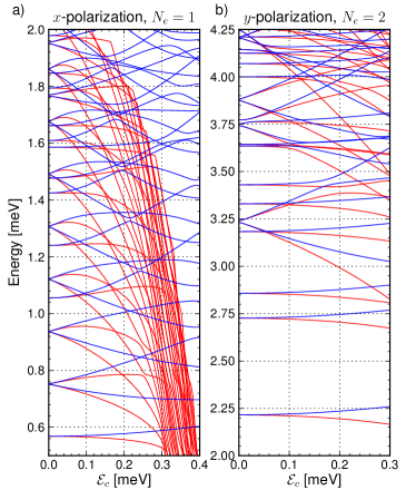
Figure 1: Energy spectra for the lowest $\sim 60$ states with one electron and $x$-polarization (a) and two electrons and $y$-polarization (b). The diamagnetic $A^{2}$ term in the e-EM interaction Hamiltonian is both included (blue) and omitted (red). In (a), the system is on resonance between the one electron states $|1)_{1}$ and $|2)_{1}$ with a DGC strength of $\left|\mathcal{G}_{12}\right|=0.290$ and $\hbar\omega_{p}=0.185$ meV. In (b), the system is on resonance between the two electron states $|1)_{2}$ and $|5)_{2}$ with a DGC strength of $\left|\mathcal{G}_{15}\right|=0.987$ and $\hbar\omega_{p}=1.025$ meV. As can be seen from the figure, omitting the $A^{2}$ term does give accurate results for small $\mathcal{E}_{c}$, while for large $\mathcal{E}_{c}$ the energy spectrum takes a steep dive downwards. This dive also takes place in the two electron case, however it can’t be seen in the chosen range of $\mathcal{E}_{c}$. There is no physical significance in these dives since the results are highly divergent in those areas.

To get an estimate of the numerical truncation errors we look at the relative variation of the energy of state $|\breve{\alpha})$ defined as

$$R^{(\alpha)}_{ij}\equiv\left|\frac{E_{i}^{(\alpha)}-E_{j}^{(\alpha)}}{E_{i}^{(\alpha)}}\right|$$ (37)

where $E_{i}^{(\alpha)}$ is the energy of state $|\breve{\alpha})$ and $i$ refers to a specific parameter related to the size of the truncated Fock space. For example $i$ can be $N_{\textrm{mes}}$, $N_{\textrm{mesT}}$ or $N_{\textrm{EM}}$. Typically, $j$ is the maximum value of that parameter which can be used to obtain the numerical output in a reasonable computing time. We vary $i$ and check the converge of the results. When changing the parameters $i$ and $j$, all other accuracy parameters are kept constant. We also define the maximum error of the $N$ lowest states as

$$R_{ij}^{\text{max}}\equiv\max_{\beta\in[1,N]}R^{(\beta)}_{ij}\ .$$ (38)

The value we choose for $N$ depends on what we intend to use the states for, once we have obtained them. For calculating electron transport using the generalized master equation $64$ states are typically used, so that is the value we will use for $N$ Gudmundsson et al. (2012). Our criteria for convergent results is that the error is not visible on a graph such as in Figure 1. This condition translates into a maximum relative error of $\sim 10^{-3}$.

Figure 2 shows the relative error in the energy spectrum for one electron due to the finite value of $N_{\textrm{mesT}}$, that is the error due to the truncation of the electron part of the joint electron-photon Fock space basis. From the figure we see that for $N_{\textrm{mesT}}=200$, results are convergent up to $\left|\mathcal{G}_{12}\right|\mathcal{E}_{c}/\hbar\omega_{p}\simeq 0.6$ for $x$-polarization and $\left|\mathcal{G}_{15}\right|\mathcal{E}_{c}/\hbar\omega_{p}\simeq 0.7$ for $y$-polarization. From the figure we also see that the error rises very rapidly for small $\mathcal{E}_{c}$ but as $\mathcal{E}_{c}$ becomes a considerable fraction of $\hbar\omega_{p}$, the error increases much slower.

Figure 3 shows the relative error due to the finite value of $N_{\textrm{mesT}}$ for two electrons and both polarizations. For $N_{\textrm{mesT}}=200$, the results are convergent up to $\left|\mathcal{G}_{12}\right|\mathcal{E}_{c}/\hbar\omega_{p}\simeq 0.3$ for $x$-polarization and $\left|\mathcal{G}_{15}\right|\mathcal{E}_{c}/\hbar\omega_{p}\simeq 0.3$ for $y$-polarization. The same convergence calculations for $3$ electrons (not shown here) gives convergent results for $\left|\mathcal{G}_{13}\right|\mathcal{E}_{c}/\hbar\omega_{p}\simeq 0.25$ for $x$-polarization and $\left|\mathcal{G}_{15}\right|\mathcal{E}_{c}/\hbar\omega_{p}\simeq 0.25$ for $y$-polarization.

Figure 4 shows the relative error due to the finite value of $N_{\textrm{EM}}$, that is the truncation of the photon part of the joint electron-photon Fock space basis. From the figure we see that a modest value of $N_{\textrm{EM}}=20$ is enough for the error to be $3-12$ orders of magnitude smaller than the $N_{\textrm{mesT}}$ truncation error shown in figures 2 and 3. The results in Figure 4 are for one electron but the two and three electron cases (not shown here) exhibit the same behavior. The reason for this faster convergence w.r.t $N_{\textrm{EM}}$ is most likely that the electronic energy spectrum is much more dense, with a high amount of energy crossings/anti-crossings, which requires a larger basis.

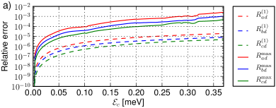
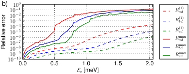
Figure 2: Convergence calculations with respect to $N_{\textrm{mesT}}$ for $x$-polarization (a) and $y$-polarization (b). In (a), the system is on resonance between the one electron states $|1)_{1}$ and $|2)_{1}$ giving $\hbar\omega_{p}=0.185$ meV and $\left|\mathcal{G}_{12}\right|=0.290$. The results are convergent up to $\mathcal{E}_{c}\simeq 0.37$ or $\left|\mathcal{G}_{12}\right|\mathcal{E}_{c}/\hbar\omega_{p}\simeq 0.6$. In (b) the system is on resonance between the one electron states $|1)_{1}$ and $|5)_{1}$ giving $\hbar\omega_{p}=1.03$ meV and $\left|\mathcal{G}_{15}\right|=0.701$. The results are convergent up to $\mathcal{E}_{c}\simeq 1.05$ or $\left|\mathcal{G}_{15}\right|\mathcal{E}_{c}/\hbar\omega_{p}\simeq 0.7$. For this run we have $a=100$, $b=150$, $c=200$ and $d=250$ (see equations 37 and 38 for definition). The maximum number of photons is kept constant at $N_{\textrm{EM}}=20$.

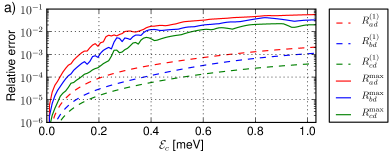
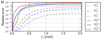
Figure 3: Convergence calculations with respect to $N_{\textrm{mesT}}$ for $x$-polarization (a) and $y$-polarization (b). In (a), the system is on resonance between the two electron states $|1)_{2}$ and $|2)_{2}$ giving $\hbar\omega_{p}=0.516$ meV and $\left|\mathcal{G}_{12}\right|=0.648$. The results are convergent up to $\mathcal{E}_{c}\simeq 0.25$ or $\left|\mathcal{G}_{12}\right|\mathcal{E}_{c}/\hbar\omega_{p}\simeq 0.3$. In (b) the system is on resonance between the two electron states $|1)_{2}$ and $|5)_{2}$ giving $\hbar\omega_{p}=1.03$ meV and $\left|\mathcal{G}_{15}\right|=0.987$. The results are convergent up to $\mathcal{E}_{c}\simeq 0.25$ or $\left|\mathcal{G}_{15}\right|\mathcal{E}_{c}/\hbar\omega_{p}\simeq 0.24$. For this run we have $a=100$, $b=150$, $c=200$ and $d=250$ (see equations 37 and 38 for definition). Other accuracy parameters are $N_{\textrm{ses}}=50$ and $N_{\textrm{EM}}=20$.

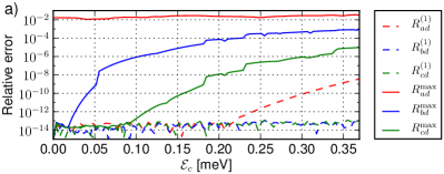
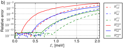
Figure 4: Convergence calculations with respect to $N_{\textrm{EM}}$ for $x$-polarization (a) and $y$-polarization (b). Values of $\hbar\omega_{p}$ and $\left|\mathcal{G}_{\lambda\kappa}\right|$ are the same as in Figure 2 for both polarizations. We can see that for $N_{EM}=20$ (green), the results are acceptable for the whole range of $\mathcal{E}_{c}$ considered. For this run we have $a=10$, $b=15$, $c=20$ and $d=25$ (see equations 37 and 38 for definition). The electron state number is kept constant at $N_{\textrm{mesT}}=200$.

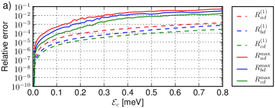
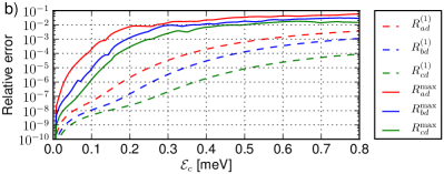
Figure 5: Convergence calculations for two electrons with respect to $N_{\textrm{mesT}}$ for $x$-polarization (a) and $y$-polarization (b). For both polarizations, the system is off resonance with $\hbar\omega_{p}=0.4$ meV. In both cases, the results are convergent up to $\mathcal{E}_{c}\simeq 0.26$ or $\mathcal{E}_{c}/\hbar\omega_{p}\simeq 0.65$. For this run we have $a=100$, $b=150$, $c=200$ and $d=250$ (see equations 37 and 38 for definition). Other accuracy parameters are $N_{\textrm{ses}}=50$ and $N_{\textrm{EM}}=20$.

Although in this paper we have put the photon frequency on resonance between two electronic states, we are in no way forced to do so (see Ref. Jonasson et al. (2012)). This motivates us to investigate convergence for a system that is off resonance. Figure 5 shows convergence calculations for a system that is off resonance and contains two electrons. From the figure we see that the results are convergent up to $\mathcal{E}_{c}/\hbar\omega_{p}\simeq 0.65$ for both $x$ and $y$ polarizations. The reason we use the ratio $\mathcal{E}_{c}/\hbar\omega_{p}$ rather than $\left|\mathcal{G}_{\kappa\lambda}\right|\mathcal{E}_{c}/\hbar\omega_{p}$ is that when the system is off resonance, the concept of active states $|\lambda)$ and $|\kappa)$ has no meaning.

VI Concluding remarks

We have described a rigorous method to compute the many-body states of a multi level Coulomb interacting electronic system which also interacts with a single-mode quantized EM field. The model is exact in the sense that the only approximations are the finite size of the single- and many-body bases and the finite size of grids on which single-electron eigenfunctions are stored. The convergence with respect to these parameters is carefully controlled.

Due to the exact numerical nature of the model, calculations for arbitrarily strong photon-matter interaction can in principle be performed with a big enough basis. Numerical results show that the main bottleneck is the large number of electron states needed in the joint photon-electron many-body basis. Convergence with respect to the number of photon states is much faster where $\sim 20$ states are sufficient to guarantee numerical error that is $3-12$ orders of magnitude smaller than the error caused by the electronic basis truncation with $\sim 200$ states. We have found that including the diamagnetic photon-electron interaction term drastically improves convergence when the electron-photon coupling strength is considerable in size to the single photon energy (ultrastrong coupling regime). Without the diamagnetic term, the model shows unphysical behavior in the ultrastrong coupling regime due to divergent results.