Towards a Mathematical Theory of Super-Resolution

Abstract

This paper develops a mathematical theory of super-resolution. Broadly speaking, super-resolution is the problem of recovering the fine details of an object—the high end of its spectrum—from coarse scale information only—from samples at the low end of the spectrum. Suppose we have many point sources at unknown locations in $[0,1]$ and with unknown complex-valued amplitudes. We only observe Fourier samples of this object up until a frequency cut-off $f_{c}$. We show that one can super-resolve these point sources with infinite precision—i.e. recover the exact locations and amplitudes—by solving a simple convex optimization problem, which can essentially be reformulated as a semidefinite program. This holds provided that the distance between sources is at least $2/f_{c}$. This result extends to higher dimensions and other models. In one dimension for instance, it is possible to recover a piecewise smooth function by resolving the discontinuity points with infinite precision as well. We also show that the theory and methods are robust to noise. In particular, in the discrete setting we develop some theoretical results explaining how the accuracy of the super-resolved signal is expected to degrade when both the noise level and the super-resolution factor vary.

Keywords. Diffraction limit, deconvolution, stable signal recovery, sparsity, sparse spike trains, $\ell_{1}$ minimization, dual certificates, interpolation, super-resolution, semidefinite programming..

1 Introduction

1.1 Super-resolution

Super-resolution is a word used in different contexts mainly to design techniques for enhancing the resolution of a sensing system. Interest in such techniques comes from the fact that there usually is a physical limit on the highest possible resolution a sensing system can achieve. To be concrete, the spatial resolution of an imaging device may be measured by how closely lines can be resolved. For an optical system, it is well known that resolution is fundamentally limited by diffraction. In microscopy, this is called the Abbe diffraction limit and is a fundamental obstacle to observing sub-wavelength structures. This is the reason why resolving sub-wavelength features is a crucial challenge in fields such as astronomy [32], medical imaging [22], and microscopy [28]. In electronic imaging, limitations stem from the lens and the size of the sensors, e. g. pixel size. Here, there is an inflexible limit to the effective resolution of a whole system due to photon shot noise which degrades image quality when pixels are made smaller. Some other fields where it is desirable to extrapolate fine scale details from low-resolution data—or resolve sub-pixel details—include spectroscopy [23], radar [29], non-optical medical imaging [25] and geophysics [26]. For a survey of super-resolution techniques in imaging, see [30] and the references therein.

This paper is about super-resolution, which loosely speaking is the process whereby the fine scale structure of an object is retrieved from coarse scale information only. A useful mathematical model may be of the following form: start with an object $x(t_{1},t_{2})$ of interest, a function of two spatial variables, and the point-spread function $h(t_{1},t_{2})$ of an optical instrument. This instrument acts as a filter in the sense that we may observe samples from the convolution product

$$y(t_{1},t_{2})=(x*h)(t_{1},t_{2}).$$

In the frequency domain, this equation becomes

$$\hat{y}(\omega_{1},\omega_{2})=\hat{x}(\omega_{1},\omega_{2})\hat{h}(\omega_{1},\omega_{2}),$$ (1.1)

where $\hat{x}$ is the Fourier transform of $x$, and $\hat{h}$ is the modulation transfer function or simply transfer function of the instrument. Now, common optical instruments act as low-pass filters in the sense that their transfer function $\hat{h}$ vanishes for all values of $\omega$ obeying $|\omega|\geq\Omega$ in which $\Omega$ is a frequency cut-off; that is,

$$|\omega|:=\sqrt{\omega_{1}^{2}+\omega_{2}^{2}}>\Omega\quad\Rightarrow\quad\hat{h}(\omega_{1},\omega_{2})=0.$$

In microscopy with coherent illumination, the bandwidth $\Omega$ is given by $\Omega=2\pi\text{NA}/\lambda$ where NA is the numerical aperture and $\lambda$ is the wavelength of the illumination light. For reference, the transfer function in this case is simply the indicator function of a disk and the point-spread function has spherical symmetry and a radial profile proportional to the ratio between the Bessel function of the first order and the radius. In microscopy with incoherent light, the transfer function is the Airy function and is proportional to the square of the coherent point-spread function. Regardless, the frequency cut-off induces a physical resolution limit which is roughly inversely proportional to $\Omega$ (in microscopy, the Rayleigh resolution distance is defined to be $0.61\times 2\pi/\Omega$).

Figure 1: Schematic illustration of the super-resolution problem in the spatial domain. (a) Highly resolved signal. (b) Low-pass version of signal in (a). Super-resolution is about recovering the signal in (a) by deconvolving the data in (b).

Figure 2: Schematic illustration of the super-resolution problem in the frequency domain. (a) Real part of the Fourier transform in Figure 1. (b) In red, portion of the observed spectrum. Super-resolution is about extrapolating the red fragment to recover the whole curve.

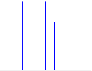
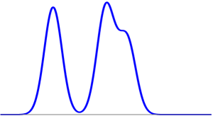
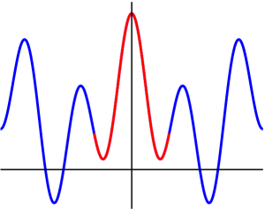
The daunting and ill-posed super-resolution problem then consists in recovering the fine-scale or, equivalently, the high-frequency features of $x$ even though they have been killed by the measurement process. This is schematically represented in Figure 1, which shows a highly resolved signal together with a low-resolution of the same signal obtained by convolution with a point-spread function. Super-resolution aims at recovering the fine scale structure on the left from coarse scale features on the right. Viewed in the frequency domain, super-resolution is of course the problem of extrapolating the high-end and missing part of the spectrum from the low-end part, as seen in Figure 2. For reference, this is very different from a typical compressed sensing problem [6] in which we wish to interpolate—and not extrapolate—the spectrum.

This paper develops a mathematical theory of super-resolution, which is not developed at all despite the abundance of empirical work in this area, see Section 1.8 for some references. Our theory takes multiple forms but a simple and appealing incarnation is as follows. Suppose we wish to super-resolve a spike-train signal as in Figure 1, namely, a superposition of pointwise events. Our main result is that we can recover such a signal exactly from low-frequency samples by tractable convex optimization in which one simply minimizes the continuous analog to the $\ell_{1}$ norm for discrete signals subject to data constraints. This holds as long as the spacing between the spikes is on the order of the resolution limit. Furthermore, the theory shows that this procedure is robust in the sense that it degrades smoothly when the measurements are contaminated with noise. In fact, we shall quantify quite precisely the error one can expect as a function of the size of the input noise and of the resolution one wishes to achieve.

1.2 Models and methods

For concreteness, consider a continuous-time model in which the signal of interest is a weighted superposition of spikes

$$x=\sum_{j}a_{j}\delta_{t_{j}},$$ (1.2)

where $\{t_{j}\}$ are locations in $[0,1]$ and $\delta_{\tau}$ is a Dirac measure at $\tau$. The amplitudes $a_{j}$ may be complex valued. Expressed differently, the signal $x$ is an atomic measure on the unit interval putting complex mass at time points $t_{1}$, $t_{2}$, $t_{3}$ and so on. The information we have available about $x$ is a sample of the lower end of its spectrum in the form of the lowest $2f_{c}+1$ Fourier series coefficients ($f_{c}$ is an integer):

$$y(k)=\int_{0}^{1}e^{-i2\pi kt}x(\text{d}t)=\sum_{j}a_{j}e^{-i2\pi kt_{j}},\quad k\in\mathbb{Z},\,\left|k\right|\leq f_{c}.$$ (1.3)

For simplicity, we shall use matrix notations to relate the data $y$ and the object $x$ and will write (1.3) as $y=\mathcal{F}_{n}\,x$ where $\mathcal{F}_{n}$ is the linear map collecting the lowest $n=2f_{c}+1$ frequency coefficients. It is important to bear in mind that we have chosen this model mainly for ease of exposition. Our techniques can be adapted to settings where the measurements are modeled differently, e. g. by sampling the convolution of the signal with different low-pass kernels. The important element is that just as before, the frequency cut-off induces a resolution limit inversely proportional to $f_{c}$; below we set $\lambda_{c}=1/f_{c}$ for convenience.

To recover $x$ from low-pass data we shall find, among all measures fitting the observations, that with lowest total variation. The total variation of a complex measure (see Section A in the Appendix for a rigorous definition) can be interpreted as being the continuous analog to the $\ell_{1}$ norm for discrete signals. In fact, with $x$ as in (1.2), $\left|\left|x\right|\right|_{\text{TV}}$ is equal to the $\ell_{1}$ norm of the amplitudes $\left|\left|a\right|\right|_{1}=\sum_{j}|a_{j}|$. Hence, we propose solving the convex program

$$\min_{\tilde{x}}\left|\left|\tilde{x}\right|\right|_{\text{TV}}\quad\text{subject to}\quad\mathcal{F}_{n}\,\tilde{x}=y,$$ (1.4)

where the minimization is carried out over the set of all finite complex measures $\tilde{x}$ supported on $[0,1]$. Our first result shows that if the spikes or atoms are sufficiently separated, at least $2\,\lambda_{c}$ apart, the solution to this convex program is exact.

Definition 1.1 (Minimum separation)

Let $\mathbb{T}$ be the circle obtained by identifying the endpoints on $[0,1]$ and $\mathbb{T}^{d}$ the $d$-dimensional torus. For a family of points $T\subset\mathbb{T}^{d}$, the minimum separation is defined as the closest distance between any two elements from $T$,

$$\Delta(T)=\inf_{(t,t^{\prime})\in T\,:\,t\neq t^{\prime}}\,\,|t-t^{\prime}|,$$ (1.5)

where $|t-t^{\prime}|$ is the $\ell_{\infty}$ distance (maximum deviation in any coordinate). To be clear, this is the wrap-around distance so that for $d=1$, the distance between $t=0$ and $t^{\prime}=3/4$ is equal to $1/4$.

Theorem 1.2

Let $T=\{t_{j}\}$ be the support of $x$. If the minimum distance obeys

$$\Delta(T)\geq{2}\,/{f_{c}}:=2\,\lambda_{c},$$ (1.6)

then $x$ is the unique solution to (1.4). This holds with the proviso that $f_{c}\geq 128$. If $x$ is known to be real-valued, then the minimum gap can be lowered to $1.87\,\lambda_{c}$.

We find this result particularly unexpected. The total-variation norm makes no real assumption about the structure of the signal. Yet, not knowing that there are any spikes, let alone how many there are, total-variation minimization locates the position of those spikes with infinite precision! Even if we knew that (1.4) returned a spike train, there is no reason to expect that the locations of the spikes would be infinitely accurate from coarse scale information only. In fact, one would probably expect the fitted locations to deviate at least a little from the truth. This is not what happens.

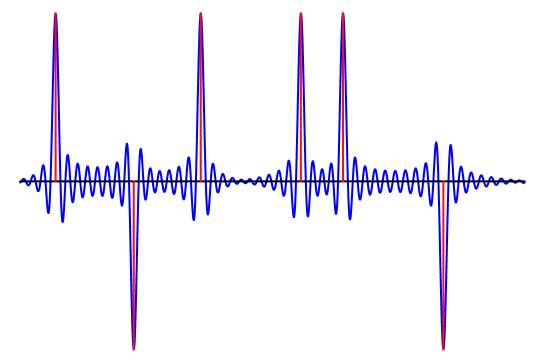
The theorem does not depend on the amplitudes and applies to situations where we have both very large and very small spikes. The information we have about $x$ is equivalent to observing the projection of $x$ onto its low-frequency components, i.e. the constraint in (1.4) is the same as $\mathcal{P}_{n}\tilde{x}=\mathcal{P}_{n}x$, where $\mathcal{P}_{n}=\mathcal{F}_{n}^{*}\mathcal{F}_{n}$. As is well known, this projection is the convolution with the Dirichlet kernel, which has slowly decaying side lobes. Hence, the theorem asserts that total-variation minimization will pull out the small spikes even though they may be completely buried in the side lobes of the large ones as shown in Figure 3. To be sure, by looking at the curves in Figure 3, it seems a priori impossible to tell how many spikes there are or roughly where they might be.

Figure 3: Low-frequency projection of a signal corresponding to a signal with three (left) and seven (right) spikes. The blue curve represents the available data while the red ticks represent the unknown locations and relative amplitudes of the spikes. The locations of the spikes obey the condition of Theorem 1.2. Yet, by looking at the curves, it seems a priori impossible to tell how many spikes there are or roughly where they might be.

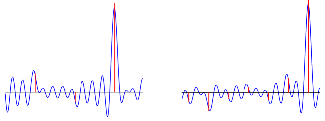
An interesting aspect of this theorem is that it cannot really be tested numerically. Indeed, one would need a numerical solver with infinite precision to check that total-variation minimization truly puts the spikes at exactly the right locations. Although this is of course not available, Section 4 shows how to solve the minimum total-variation problem (1.4) by using ideas from semidefinite programming and allowing recovery of the support with very high precision. Also, we demonstrate through numerical simulations in Section 5 that Theorem 1.2 is fairly tight in the sense that a necessary condition is a separation of at least $\lambda_{c}=1/f_{c}$.

Viewed differently, one can ask: how many spikes can be recovered from $n=2f_{c}+1$ low-frequency samples? The answer given by Theorem 1.2 is simple. At least $n/4$ provided we have the minimum separation discussed above. A classical argument shows that any method whatsoever would at least need two samples per unknown spike so that the number of spikes cannot exceed half the number of samples, i. e. $n/2$. This is another way of showing that the theorem is reasonably tight.

1.3 Super-resolution in higher dimensions

Our results extend to higher dimensions and reveal the same dependence between the minimum separation and the measurement resolution as in one dimension. For concreteness, we discuss the $2$-dimensional setting and emphasize that the situation in $d$ dimensions is similar. Here, we have a measure

$$x=\sum_{j}a_{j}\delta_{t_{j}},$$

as before but in which the $t_{j}\in[0,1]^{2}$. We are given information about $x$ in the form of low-frequency samples of the form

$$y(k)=\int_{[0,1]^{2}}e^{-i2\pi\langle k,t\rangle}x(\text{d}t)=\sum_{j}a_{j}e^{-i2\pi\langle k,t_{j}\rangle},\quad k=(k_{1},k_{2})\in\mathbb{Z}^{2},\,\left|k_{1}\right|,\left|k_{2}\right|\leq f_{c}.$$ (1.7)

This again introduces a physical resolution of about $\lambda_{c}=1/f_{c}$. In this context, we may think of our problem as imaging point sources in the 2D plane—such as idealized stars in the sky—with an optical device with resolution about $\lambda_{c}$—such as a diffraction limited telescope. Our next result states that it is possible to locate the point sources without any error whatsoever if they are separated by a distance of $2.38\,\lambda_{c}$ simply by minimizing the total variation.

Theorem 1.3

Let $T=\{t_{j}\}\subset[0,1]^{2}$ identified with $\mathbb{T}^{2}$ be the support of $x$ obeying the separation condition

$$\Delta(T)\geq{2.38}\,/{f_{c}}={2.38}\,\lambda_{c}.$$ (1.8)

Then if $x$ is real valued, it is the unique minimum total-variation solution among all real objects obeying the data constraints (1.7). Hence, the recovery is exact. For complex measures, the same statement holds but with a slightly different constant.

Whereas we have tried to optimize the constant in one dimension, we have not really attempted to do so here in order to keep the proof reasonably short and simple. Hence, this theorem is subject to improvement.

Theorem 1.3 is proved for real-valued measures in Section C of the Appendix. However, the proof techniques can be applied to higher dimensions and complex measures almost directly. In details, suppose we observe the discrete Fourier coefficients of a $d$-dimensional object at $k=(k_{1},\ldots,k_{d})\in\mathbb{Z}^{d}$ corresponding to low frequencies $0\leq|k_{1}|,\ldots,|k_{d}|\leq f_{c}$. Then the minimum total-variation solution is exact provided that the minimum distance obeys $\Delta(T)\geq c_{d}\,\lambda_{c}$, where $c_{d}$ is some positive numerical constant depending only on the dimension. Finally, as the proof makes clear, extensions to other settings, in which one observes Fourier coefficients if and only if the $\ell_{2}$ norm of $k$ is less or equal to a frequency cut-off, are straightforward.

1.4 Discrete super-resolution

Our continuous theory immediately implies analogous results for finite signals. Suppose we wish to recover a discrete signal $x\in\mathbb{C}^{N}$ from low-frequency data. Just as before, we could imagine collecting low-frequency samples of the form

$$y_{k}=\sum_{t=0}^{N-1}x_{t}e^{-i2\pi kt/N},\quad|k|\leq f_{c};$$ (1.9)

the connection with the previous sections is obvious since $x$ might be interpreted as samples of a discrete signal on a grid $\{t/N\}$ with $t=0,1,\ldots,N-1$. In fact, the continuous-time setting is the limit of infinite resolution in which $N$ tends to infinity while the number of samples remains constant ($f_{c}$ fixed). Instead, we can choose to study the regime in which the ratio between the actual resolution of the signal $1/N$ and the resolution of the data defined as $1/f_{c}$ is constant. This gives the corollary below.

Corollary 1.4

Let $T\subset\{0,1,\ldots,N-1\}$ be the support of $\{x_{t}\}_{t=0}^{N-1}$ obeying

$$\min_{t,t^{\prime}\in T:t\neq t^{\prime}}\frac{1}{N}\left|t-t^{\prime}\right|\geq{2}\,\lambda_{c}={2}\,/{f_{c}}.$$ (1.10)

Then the solution to

$$\min\left|\left|\tilde{x}\right|\right|_{1}\quad\text{subject to}\quad F_{n}\tilde{x}=y$$ (1.11)

in which $F_{n}$ is the partial Fourier matrix in (1.9) is exact.

1.5 The super-resolution factor

In the discrete framework, we wish to resolve a signal on a fine grid with spacing $1/N$. However, we only observe the lowest $n=2f_{c}+1$ Fourier coefficients so that in principle, one can only hope to recover the signal on a coarser grid with spacing only $1/n$ as shown in Figure 4. Hence, the factor $N/n$, or equivalently, the ratio between the spacings in the coarse and fine grids, can be interpreted as a super-resolution factor (SRF). Below, we set

$$\text{SRF}=N/n\approx N/2f_{c};$$ (1.12)

when the SRF is equal to 5 as in the figure, we are looking for a signal at a resolution 5 times higher than what is stricto senso permissible. One can then recast Corollary 1.4 as follows: if the nonzero components of $\{x_{t}\}_{t=0}^{N-1}$ are separated by at least $4\times\text{SRF}$, perfect super-resolution via $\ell_{1}$ minimization occurs.

Figure 4: Fine grid with spacing $1/N$. We only observe frequencies between $-f_{c}$ and $f_{c}$, $f_{c}/N\approx\frac{1}{2}\text{SRF}^{-1}$, so that the highest frequency sine wave available has wavelength $1/f_{c}=\lambda_{c}$. These data only allow a Nyquist sampling rate of $\lambda_{c}/2\approx 1/n$. In this sense, we can interpret the super-resolution factor $N/n$ as the ratio between these two resolutions.

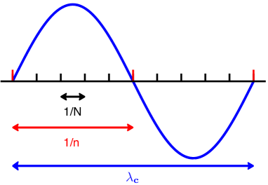
The reason for introducing the SRF is that with inexact data, we obviously cannot hope for infinite resolution. Indeed, noise will ultimately limit the resolution one can ever hope to achieve and, therefore, the question of interest is to study the accuracy one might expect from a practical super-resolution procedure as a function of both the noise level and the SRF.

1.6 Stability

To discuss the robustness of super-resolution methods vis a vis noise, we examine in this paper the discrete setting of Section 1.4. In this setup, we could certainly imagine studying a variety of deterministic and stochastic noise models, and a variety of metrics in which to measure the size of the error. For simplicity, we study a deterministic scenario in which the projection of the noise onto the signal space has bounded $\ell_{1}$ norm but is otherwise arbitrary and can be adversarial. The observations are consequently of the form

$$y=F_{n}x+w,\quad\frac{1}{N}\,\left|\left|F_{n}^{\ast}w\right|\right|_{1}\leq\delta$$ (1.13)

for some $\delta\geq 0$, where $F_{n}$ is as before. Letting $P_{n}$ be the orthogonal projection of a signal onto the first $n$ Fourier modes, $P_{n}=\frac{1}{N}F_{n}^{*}F_{n}$, we can view (1.13) as an input noise model since with $w=F_{n}z$, we have

$$y=F_{n}(x+z),\quad\left|\left|z\right|\right|_{1}\leq\delta,\,z=P_{n}z.$$

Another way to write this model with arbitrary input noise $z\in\mathbb{C}^{N}$ is

$$y=F_{n}(x+z),\quad\left|\left|P_{n}z\right|\right|_{1}\leq\delta$$

since the high-frequency part of $z$ is filtered out by the measurement process. Finally, with $s={N}^{-1}F_{n}^{*}y$, (1.13) is equivalent to

$$s=P_{n}x+P_{n}z,\quad\left|\left|P_{n}z\right|\right|_{1}\leq\delta.$$ (1.14)

In words, we observe a low-pass version of the signal corrupted with an additive low-pass error whose $\ell_{1}$ norm is at most $\delta$. In the case where $n=N$, $P_{n}=I$, and our model becomes

$$s=x+z,\quad\|z\|_{1}\leq\delta.$$

In this case, one cannot hope for a reconstruction $\hat{x}$ with an error in the $\ell_{1}$ norm less than the noise level $\delta$. We now wish to understand how quickly the recovery error deteriorates as the super-resolution factor increases.

We propose studying the relaxed version of the noiseless problem (1.11)

$$\min_{\tilde{x}}\,\left|\left|\tilde{x}\right|\right|_{1}\quad\text{subject to}\quad\left|\left|P_{n}\tilde{x}-s\right|\right|_{1}\leq\delta.$$ (1.15)

We show that this recovers $x$ with a precision inversely proportional to $\delta$ and to the square of the super-resolution factor.

Theorem 1.5

Assume that $x$ obeys the separation condition (1.6). Then with the noise model (1.14), the solution $\hat{x}$ to (1.15) obeys

$$\left|\left|\hat{x}-x\right|\right|_{1}\leq C_{0}\,\text{\em SRF}^{2}\,\delta,$$ (1.16)

for some positive constant $C_{0}$.

This theorem, which shows the simple dependence upon the super-resolution factor and the noise level, is proved in Section 3. Clearly, plugging in $\delta=0$ in (1.16) gives Corollary 1.4.

Versions of Theorem 1.5 hold in the continuous setting as well, where the locations of the spikes are not assumed to lie on a given fine grid but can take on a continuum of values. The arguments are more involved than those needed to establish (1.16) and we leave a detailed study to a future paper.

1.7 Sparsity and stability

Researchers in the field know that super-resolution under sparsity constraints alone is hopelessly ill posed. In fact, without a minimum distance condition, the support of sparse signals can be very clustered, and clustered signals can be nearly completely annihilated by the low-pass sensing mechanism. The extreme ill-posedness can be understood by means of the seminal work of Slepian [36] on discrete prolate spheroidal sequences. This is surveyed in Section 3.2 but we give here a concrete example to drive this point home.

To keep things simple, we consider the ‘analog version’ of (1.14) in which we observe

$$s=\mathcal{P}_{W}(x+z);$$

$\mathcal{P}_{W}(x)$ is computed by taking the discrete-time Fourier transform $y(\omega)=\sum_{t\in\mathbb{Z}}x_{t}e^{-i2\pi\omega t}$, $\omega\in[-1/2,1/2],$ and discarding all ‘analog’ frequencies outside of the band $[-W,W]$. If we set

$$2W=n/N=1/\text{SRF},$$

we essentially have $\mathcal{P}_{W}=P_{n}$ where the equality is true in the limit where $N\rightarrow\infty$ (technically, $\mathcal{P}_{W}$ is the convolution with the sinc kernel while $P_{n}$ uses the Dirichlet kernel). Set a mild level of super-resolution to fix ideas,

$$\text{SRF}=4.$$

Now the work of Slepian shows that there is a $k$-sparse signal supported on $[0,\ldots,k-1]$ obeying

$$\mathcal{P}_{W}x=\lambda\,x,\quad\lambda\approx 5.22\,\sqrt{k+1}\,e^{-3.23\left(k+1\right)}.$$ (1.17)

For $k=48$,

$$\lambda\leq 7\times 10^{-68}.$$ (1.18)

Even knowing the support ahead of time, how are we going to recover such signals from noisy measurements? Even for a very mild super-resolution factor of just $\text{SRF}=1.05$ (we only seek to extend the spectrum by 5%), (1.17) becomes

$$\mathcal{P}_{W}x=\lambda\,x,\quad\lambda\approx 3.87\,\sqrt{k+1}\,e^{-0.15\left(k+1\right)},$$ (1.19)

which implies that there exists a unit-norm signal with at most $256$ consecutive nonzero entries such that $\left|\left|\mathcal{P}_{W}x\right|\right|_{2}\leq 1.2\times 10^{-15}$. Of course, as the super-resolution factor increases, the ill-posedness gets worse. For large values of SRF, there is $x$ obeying (1.17) with

$$\log\lambda\approx-(0.4831+2\log(\text{SRF}))k.$$ (1.20)

It is important to emphasize that this is not a worst case analysis. In fact, with $k=48$ and $\text{SRF}=4$, Slepian shows that there is a large dimensional subspace of signals supported on $\mathbb{C}^{k}$ spanned by orthonormal eigenvectors with eigenvalues of magnitudes nearly as small as (1.18).

1.8 Comparison with related work

The use of $\ell_{1}$ minimization for the recovery of sparse spike trains from noisy bandlimited measurements has a long history and was proposed in the 1980s by researchers in seismic prospecting [8, 27, 35]. For finite signals and under the rather restrictive assumption that the signal is real valued and nonnegative, [20] and [12] prove that $k$ spikes can be recovered from $2k+1$ Fourier coefficients by this method. The work [9] extends this result to the continuous setting by using total-variation minimization. In contrast, our results require a minimum distance between spikes but allow for arbitrary complex amplitudes, which is crucial in applications. The only theoretical guarantee we are aware of concerning the recovery of spike trains with general amplitudes is very recent and due to Kahane [24]. Kahane offers variations on compressive sensing results in [6] and studies the reconstruction of a function with lacunary Fourier series coefficients from its values in a small contiguous interval, a setting that is equivalent to that of Corollary 1.4 when the size $N$ of the fine grid tends to infinity. With our notation, whereas we require a minimum distance equal to $4\times\text{SRF}$, this work shows that a minimum distance of $10\times\text{SRF}\sqrt{\log\text{SRF}}$ is sufficient for exact recovery. Although the log factor might seem unimportant at first glance, it in fact precludes extending Kahane’s result to the continuous setting of Theorem 1.2. Indeed, by letting the resolution factor tend to infinity so as to approach the continuous setting, the spacing between consecutive spikes would need to tend to infinity as well.

As to results regarding the robustness of super-resolution in the presence of noise, Donoho [10] studies the modulus of continuity of the recovery of a signed measure on a discrete lattice from its spectrum on the interval $\left[-f_{c},f_{c}\right]$, a setting which is also equivalent to that of Corollary 1.4 when the size $N$ of the fine grid tends to infinity. More precisely, if the support of the measure is constrained to contain at most $\ell$ elements in any interval of length $2/(\ell\,f_{c})$, then the modulus of continuity is of order $O\left(\text{SRF}^{2\ell+1}\right)$ as SRF grows to infinity (note that for $\ell=1$ the constraint reduces to a minimum distance condition between spikes, which is comparable to the separation condition (1.6)). This means that if the $\ell_{2}$ norm of the difference between the measurements generated by two signals satisfying the support constraints is known to be at most $\delta$, then the $\ell_{2}$ norm of the difference between the signals may be of order $O\left(\text{SRF}^{2\ell+1}\,\delta\right)$. This result suggests that, in principle, the super-resolution of spread-out signals is not hopelessly ill-conditioned. Having said this, it does not propose any practical recovery algorithm (a brute-force search for sparse measures obeying the low-frequency constraints would be computationally intractable).

Finally, we would like to mention an alternative approach to the super-resolution of pointwise events from coarse scale data. Leveraging ideas related to error correction codes and spectral estimation, [15] shows that it is possible to recover trains of Dirac distributions from low-pass measurements at their rate of innovation (in essence, the density of spikes per unit of time). This problem, however, is extraordinarily ill posed without a minimum separation assumption as explained in Sections 1.7 and 3.2. Moreover, the proposed reconstruction algorithm in [15] needs to know the number of events ahead of time, and relies on polynomial root finding. As a result, it is highly unstable in the presence of noise as discussed in [37], and in the presence of approximate sparsity. Algebraic techniques have also been applied to the location of singularities in the reconstruction of piecewise polynomial functions from a finite number of Fourier coefficients (see [1, 2, 18] and references therein). The theoretical analysis of these methods proves their accuracy up to a certain limit related to the number of measurements. Corollary 1.6 takes a different approach, guaranteeing perfect localization if there is a minimum separation between the singularities.

1.9 Connections to sparse recovery literature

Theorem 1.2 and Corollary 1.4 can be interpreted in the framework of sparse signal recovery. For instance, by swapping time and frequency, Corollary 1.4 asserts that one can recover a sparse superposition of tones with arbitrary frequencies from $n$ time samples of the form

$$y_{t}=\sum_{j=0}^{N-1}x_{j}e^{-i2\pi t\omega_{j}},\quad t=0,1,\ldots,n-1$$

where the frequencies are of the form $\omega_{j}=j/N$. Since the spacing between consecutive frequencies is not $1/n$ but $1/N$, we may have a massively oversampled discrete Fourier transform, where the oversampling ratio is equal to the super-resolution factor. In this context, a sufficient condition for perfectly super-resolving these tones is a minimum separation of $4/n$. In addition, Theorem 1.2 extends this to continuum dictionaries where tones $\omega_{j}$ can take on arbitrary real values.

In the literature, there are several conditions that guarantee perfect signal recovery by $\ell_{1}$ minimization. The results obtained from their application to our problem are, however, very weak.

• The matrix with normalized columns $f_{j}=\{e^{-i2\pi t\omega_{j}}/\sqrt{n}\}_{t=0}^{n-1}$ does not obey the restricted isometry property [7] since a submatrix composed of a very small number of contiguous columns is already very close to singular, see [36] and Section 3.2 for related claims. For example, with $N=512$ and a modest SRF equal to 4, the smallest singular value of submatrices formed by eight consecutive columns is $3.32\;10^{-5}$.

• Applying the discrete uncertainty principle proved in [11], we obtain that recovery by $\ell_{1}$ minimization succeeds as long as

  $$2\left|T\right|(N-n)<N.$$

  If $n<N/2$, i.e. $\text{SRF}>2$, this says that $|T|$ must be zero. In other words, to recover one spike, we would need at least half of the Fourier samples.

• Other guarantees based on the coherence of the dictionary yield similar results. A popular condition [39] requires that

  $$|T|<\frac{1}{2}(M^{-1}+1),$$ (1.21)

  where $M$ is the coherence of the system defined as $\max_{i\neq j}|\langle f_{i},f_{j}\rangle|$. When $N=1024$ and $\text{SRF}=4$, $M\approx 0.9003$ so that this becomes $|T|\leq 1.055$, and we can only hope to recover one spike.

There are slightly improved versions of (1.21). In [13], Dossal studies the deconvolution of spikes by $\ell_{1}$ minimization. This work introduces the weak exact recovery condition (WERC) defined as

$$\text{WERC}\left(T\right)=\frac{\beta\left(T\right)}{1-\alpha\left(T\right)},$$

where

$$\alpha(T)=\sup_{i\in T}\sum_{j\in T/\left\{i\right\}}\left|\left\langle f_{i},f_{j}\right\rangle\right|,\quad\beta(T)=\sup_{i\in T^{c}}\sum_{j\in T}\left|\left\langle f_{i},f_{j}\right\rangle\right|.$$

The condition $\text{WERC}\left(T\right)<1$ guarantees exact recovery. Considering three spikes and using Taylor expansions to bound the sine function, the minimum distance needed to ensure that $\text{WERC}\left(T\right)<1$ may be lower bounded by $24\text{SRF}^{3}/\pi^{3}-2\text{SRF}$. This is achieved by considering three spikes at $\omega\in\{0,\pm\Delta\}$, where $\Delta=(k+1/2)/n$ for some integer $k$; we omit the details. If $N=20,000$ and the number of measurements is $1,000$, this allows for the recovery of at most $3$ spikes, whereas Corollary 1.4 implies that it is possible to reconstruct at least $n/4=250$. Furthermore, the cubic dependence on the super-resolution factor means that if we fix the number of measurements and let $N\rightarrow\infty$, which is equivalent to the continuous setting of Theorem 1.2, the separation needed becomes infinite and we cannot guarantee the recovery of even two spikes.

Finally, we would also like to mention some very recent work on sparse recovery in highly coherent frames by modified greedy compressed sensing algorithms [16, 19]. Interestingly, these approaches explicitly enforce conditions on the recovered signals that are similar in spirit to our minimum distance condition. As opposed to $\ell_{1}$-norm minimization, such greedy techniques may be severely affected by large dynamic ranges (see [19]) because of the phenomenon illustrated in Figure 3. Understanding under what conditions their performance may be comparable to that of convex programming methods is an interesting research direction.

1.10 Extensions

Our results and techniques can be extended to super-resolve many other types of signals. We just outline such a possible extension. Suppose $x:[0,1]\rightarrow\mathbb{C}$ is a periodic piecewise smooth function with period 1, defined by

$$x(t)=\sum_{t_{j}\in T}\mathbf{1}_{\left(t_{j-1},t_{j}\right)}p_{j}(t);$$

on each time interval $(t_{j-1},t_{j})$, $x$ is polynomial of degree $\ell$. For $\ell=0$, we have a piecewise constant function, for $\ell=1$, a piecewise linear function and so on. Also suppose $x$ is globally $\ell-1$ times continuously differentiable (as for splines). We observe

$$y_{k}=\int_{[0,1]}x(t)\,e^{-i2\pi kt}\text{d}t\;,\;\left|k\right|\leq f_{c}.$$

The $(\ell+1)$th derivative of $x$ (in the sense of distributions) denoted by $x^{(\ell+1)}$ is an atomic measure supported on $T$ and equal to

$$x^{(\ell+1)}=\sum_{j}a_{j}\delta_{t_{j}},\quad a_{j}=p^{(\ell)}_{j+1}(t_{j})-p^{(\ell)}_{j}(t_{j}).$$

Hence, we can imagine recovering $x^{(\ell+1)}$ by solving

$$\min\|\tilde{x}^{(\ell+1)}\|_{\text{TV}}\quad\text{subject to}\quad F_{n}\tilde{x}=y.$$ (1.22)

Standard Fourier analysis gives that the $k$th Fourier coefficient of this measure is given by

$$y^{(\ell+1)}_{k}=(i2\pi k)^{\ell+1}\,y_{k},\quad k\neq 0.$$ (1.23)

Hence, we observe the Fourier coefficients of $x^{(\ell+1)}$ except that corresponding to $k=0$, which must vanish since the periodicity implies $\int_{0}^{1}x^{(\ell+1)}(\text{d}t)=0=\int_{0}^{1}x^{(j)}(t)\text{d}t$, $1\leq j\leq\ell$. Hence, it follows from Theorem 1.2 that (1.22) recovers $x^{(\ell+1)}$ exactly as long as the discontinuity points are at least $2\lambda_{c}$ apart. Because $x$ is $\ell-1$ times continuously differentiable and periodic, $x^{(\ell+1)}$ determines $x$ up to a shift in function value, equal to its mean. However, we can read the mean value of $x$ off $y_{0}=\int_{0}^{1}x(t)\text{d}t$ and, therefore, (1.22) achieves perfect recovery.

Corollary 1.6

If $T=\{t_{j}\}$ obeys (1.6), $x$ is determined exactly from $y$ by solving (1.22).

Extensions to non-periodic functions, other types of discontinuities and smoothness assumptions are straightforward.

1.11 Organization of the paper

The remainder of the paper is organized as follows. We prove our main noiseless result in Section 2. There, we introduce our techniques which involve the construction of an interpolating low-frequency polynomial. Section 3 proves our stability result and argues that sparsity constraints cannot be sufficient to guarantee stable super-resolution. Section 4 shows that (1.4) can be cast as a finite semidefinite program. Numerical simulations providing a lower bound for the minimum distance that guarantees exact recovery are presented in Section 5. We conclude the paper with a short discussion in Section 6.

2 Noiseless Recovery

This section proves the noiseless recovery result, namely, Theorem 1.2. Here and below, we write $\Delta=\Delta(T)\geq\Delta_{\text{min}}=2\,\lambda_{c}$. Also, we identify the interval $[0,1)$ with the circle $\mathbb{T}$.

2.1 Dual polynomials

In the discrete setting, the compressed sensing literature has made clear that the existence of a certain dual certificate guarantees that the $\ell_{1}$ solution is exact [6]. In the continuous setting, a sufficient condition for the success of the total-variation solution is this: for any $v\in\mathbb{C}^{|T|}$ with $|v_{j}|=1$, there exists a low-frequency trigonometric polynomial

$$q(t)=\sum_{k=-f_{c}}^{f_{c}}c_{k}e^{i2\pi kt}$$ (2.1)

obeying the following properties

$$\begin{cases}q(t_{j})=v_{j},&t_{j}\in T,\\ |q(t)|<1,&t\in\mathbb{T}\setminus T.\end{cases}$$ (2.2)

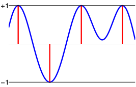
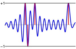
This result follows from elementary measure theory and is included in Section A of the Appendix for completeness. Constructing a bounded low-frequency polynomial interpolating the sign pattern of certain signals becomes increasingly difficult if the minimum distance separating the spikes is too small. This is illustrated in Figure 5, where we show that if spikes are very near, it would become in general impossible to find an interpolating low-frequency polynomial obeying (2.2).

Figure 5: (a) Low-frequency polynomial interpolating a sign pattern in which the support is well separated, and obeying the off-support condition (2.2). In (b), we see that if the spikes become very near, we would need a rapidly (high-frequency) interpolating polynomial in order to achieve (2.2). This is the reason why there must be a minimum separation between consecutive spikes.

2.2 Proof of Theorem 1.2

Theorem 1.2 is a direct consequence of the proposition below, which establishes the existence of a valid dual polynomial provided the elements in the support are sufficiently spaced.

Proposition 2.1

Let $v\in\mathbb{C}^{|T|}$ be an arbitrary vector obeying $|v_{j}|=1$. Then under the hypotheses of Theorem 1.2, there exists a low-frequency trigonometric polynomial (2.1) obeying (2.2).

The remainder of this section proves this proposition. Our method consists in interpolating $v$ on $T$ with a low-frequency kernel and correcting the interpolation to ensure that the derivative of the dual polynomial is zero on $T$. The kernel we employ is

$$K(t)=\left[\frac{\sin\left(\left(\frac{f_{c}}{2}+1\right)\pi t\right)}{\left(\frac{f_{c}}{2}+1\right)\sin\left(\pi t\right)}\right]^{4},\quad 0<t<1,$$ (2.3)

and $K(0)=1$. If $f_{c}$ is even, $K(t)$ is the square of the Fejér kernel which is a trigonometric polynomial with frequencies obeying $|k|\leq f_{c}/2$. As a consequence, $K$ is of the form (2.1). The careful reader might remark that the choice of the interpolation kernel seems somewhat arbitrary. In fact, one could also use the Fejér kernel or any other power of the Fejér kernel using almost identical proof techniques. We have found that the second power nicely balances the trade-off between localization in time and in frequency, and thus yields a good constant.

To construct the dual polynomial, we interpolate $v$ with both $K$ and its derivative $K^{\prime}$,

$$q(t)=\sum_{t_{j}\in T}\alpha_{j}K(t-t_{j})+\beta_{j}K^{\prime}(t-t_{j}),$$ (2.4)

where $\alpha,\beta\in\mathbb{C}^{\left|T\right|}$ are coefficient sequences. The polynomial $q$ is as in (2.1) and in order to obey $q(t_{k})=v_{k}$, we impose

$$q(t_{k})=\sum_{t_{j}\in T}\alpha_{j}K\left(t_{k}-t_{j}\right)+\beta_{j}K^{\prime}\left(t_{k}-t_{j}\right)=v_{k},\quad\forall t_{k}\in T,$$ (2.5)

whereas in order to obey $|q(t)|<1$ for $t\in T^{c}$, we impose $q^{\prime}(t_{k})=0$,

$$q^{\prime}(t_{k})=\sum_{t_{j}\in T}\alpha_{j}K^{\prime}\left(t_{k}-t_{j}\right)+\beta_{j}K^{\prime\prime}\left(t_{k}-t_{j}\right)=0,\quad\forall t_{k}\in T.$$ (2.6)

As we will see, this implies that the magnitude of $q$ reaches a local maximum at those points, which in turn can be used to show that (2.2) holds.

The proof of Proposition 2.1 consists of three lemmas, which are the object of the following section. The first one establishes that if the support is spread out, it is possible to interpolate any sign pattern exactly.

Lemma 2.2

Under the hypotheses of Proposition 2.1, there exist coefficient vectors $\alpha$ and $\beta$ obeying

$$\left|\left|\alpha\right|\right|_{\infty} \leq\alpha^{\infty}:=1+8.824\;10^{-3},$$ (2.7)

$$\left|\left|\beta\right|\right|_{\infty} \leq\beta^{\infty}:=3.294\;10^{-2}\,\lambda_{c},$$

such that (2.5)–(2.6) hold. Further, if $v_{1}=1$,

$$\operatorname{Re}{\alpha_{1}} \geq 1-8.824\;10^{-3},$$ (2.8)

$$\left|\operatorname{Im}{\alpha_{1}}\right| \leq 8.824\;10^{-3}.$$

To complete the proof, Lemmas 2.3 and 2.4 show that $|q\left(t\right)|<1$.

Lemma 2.3

Fix $\tau\in T$. Under the hypotheses of Proposition 2.1, $|q(t)|<1$ for $\left|t-\tau\right|\in(0,0.1649\,\lambda_{c}]$.

Lemma 2.4

Fix $\tau\in T$. Then under the hypotheses of Proposition 2.1, $|q(t)|<1$ for $\left|t-\tau\right|\in[0.1649\,\lambda_{c},\Delta/2]$. This can be extended as follows: letting $\tau_{+}$ be the closest spike to the right, i. e. $\tau_{+}=\min\{t\in T:t>\tau\}$. Then $\left|q(t)\right|<1$ for all $t$ obeying $0<t-\tau\leq(\tau_{+}-\tau)/2$, and likewise for the left side.

Finally, we record a useful lemma to derive stability results.

Lemma 2.5

If $\Delta\left(T\right)\geq 2.5\,\lambda_{c}$, then for any $\tau\in T$,

$$\left|q\left(t\right)\right|\leq 1-0.3353f_{c}^{2}\left(t-\tau\right)^{2},\quad\text{for all }t:\,\left|t-\tau\right|\leq 0.1649\,\lambda_{c}.$$ (2.9)

Further, for $\min_{\tau\in T}\,\left|t-\tau\right|>0.1649\,\lambda_{c}$, $\left|q\left(t\right)\right|$ is upper bounded by the right-hand side above evaluated at $0.1649\,\lambda_{c}$.

Section 2.5 describes how the proof can be adapted to obtain a slightly smaller bound on the minimum distance for real-valued signals.

2.3 Proofs of Lemmas

The proofs of the three lemmas above make repeated use of the fact that the interpolation kernel and its derivatives decay rapidly away from the origin. The intermediate result below proved in Section B of the Appendix quantifies this.

Lemma 2.6

For $\ell\in\{0,1,2,3\}$, let $K^{(\ell)}$ be the $\ell$th derivative of $K$ ($K=K^{(0)}$). For $\frac{1}{2}f_{c}^{-1}=\frac{1}{2}\lambda_{c}\leq t\leq\frac{1}{2}$, we have

$$\left|K^{(\ell)}(t)\right|\leq B_{\ell}(t)=\begin{cases}\tilde{B}_{\ell}(t)=\frac{\pi^{\ell}H_{\ell}(t)}{(f_{c}+2)^{4-\ell}\,t^{4}},\qquad&\frac{1}{2}\lambda_{c}\leq t\leq\sqrt{2}/\pi,\\ \frac{\pi^{\ell}H_{\ell}^{\infty}}{(f_{c}+2)^{4-\ell}\,t^{4}},\qquad&\sqrt{2}/\pi\leq t<\frac{1}{2},\end{cases}$$

where $H_{0}^{\infty}=1$, $H_{1}^{\infty}=4$, $H_{2}^{\infty}=18$, $H_{3}^{\infty}=77$,

$$H_{0}(t) =a^{4}(t),$$

$$H_{1}(t) =a^{4}(t)\left(2+2b(t)\right),$$

$$H_{2}(t) =a^{4}(t)\left(4+7b(t)+6b^{2}(t)\right),$$

$$H_{3}(t) =a^{4}(t)\left(8+24b(t)+30b^{2}(t)+15b^{3}(t)\right),$$

and

$$a(t) =\frac{2}{\pi\left(1-\frac{\pi^{2}t^{2}}{6}\right)},\qquad b(t)=\frac{1}{f_{c}}\,\frac{a(t)}{t}.$$

For each $\ell$, the bound on the magnitude of $B_{\ell}(t)$ is nonincreasing in $t$ and $\tilde{B}_{\ell}(\Delta-t)+\tilde{B}_{\ell}(\Delta+t)$ is increasing in $t$ for $0\leq t<\Delta/2$ if $0\leq\Delta+t\leq\sqrt{2}/\pi$.

This lemma is used to control quantities of the form $\sum_{t_{i}\in T\setminus\{\tau\}}\left|K\left(t-t_{i}\right)\right|$ ($\tau\in T$) as shown below.

Lemma 2.7

Suppose $0\in T$. Then for all $t\in[0,\Delta/2]$,

$$\sum_{t_{i}\in T\setminus\{0\}}\left|K^{\left(\ell\right)}\left(t-t_{i}\right)\right|\leq F_{\ell}\left(\Delta,t\right)=F_{\ell}^{+}(\Delta,t)+F_{\ell}^{-}(\Delta,t)+F_{\ell}^{\infty}(\Delta_{\text{\em min}}),$$

where

$$F_{\ell}^{+}(\Delta,t) =\max\left\{\max_{\Delta\leq t_{+}\leq 3\Delta_{\text{\em min}}}\,\left|K^{\left(\ell\right)}\left(t-t_{+}\right)\right|,B_{\ell}\left(3\Delta_{\text{\em min}}-t\right)\right\}+\sum_{j=2}^{20}\tilde{B}_{\ell}(j\Delta_{\text{\em min}}-t),$$

$$F_{\ell}^{-}(\Delta,t) =\max\left\{\max_{\Delta\leq t_{-}\leq 3\Delta_{\text{\em min}}}\,\left|K^{\left(\ell\right)}\left(t_{-}\right)\right|,B_{\ell}\left(3\Delta_{\text{\em min}}\right)\right\}+\sum_{j=2}^{20}\tilde{B}_{\ell}(j\Delta_{\text{\em min}}+t),$$

$$F_{\ell}^{\infty}(\Delta_{\text{\em min}}) =\frac{\kappa\,\pi^{\ell}H_{\ell}^{\infty}}{(f_{c}+2)^{4-\ell}\Delta_{\text{\em min}}^{4}},\qquad\kappa=\frac{\pi^{4}}{45}-2\sum_{j=1}^{19}\frac{1}{j^{4}}\leq 8.98\,10^{-5}.$$

Moreover, $F_{\ell}\left(\Delta,t\right)$ is nonincreasing in $\Delta$ for all $t$, and $F_{\ell}\left(\Delta_{\text{\em min}},t\right)$ is nondecreasing in $t$.

Proof We consider the sum over positive $t_{i}\in T$ first and denote by $t_{+}$ the positive element in $T$ closest to $0$. We have

$$\sum_{t_{i}\in T:\,0<t_{i}\leq 1/2}\left|K^{\left(\ell\right)}\left(t-t_{i}\right)\right|=\left|K^{\left(\ell\right)}\left(t-t_{+}\right)\right|+\sum_{t_{i}\in T\setminus\{t_{+}\}:\,0<t_{i}\leq 1/2}\left|K^{\left(\ell\right)}\left(t-t_{i}\right)\right|.$$ (2.10)

Let us assume $t_{+}<2\Delta_{\text{min}}$ (if $t_{+}>2\Delta_{\text{min}}$ the argument is very similar). Note that the assumption that $f_{c}\geq 128$ implies $21\Delta_{\text{min}}<0.33<\sqrt{2}/\pi$. By Lemma 2.6 and the minimum separation condition, this means that the second term in the right-hand side is at most

$$\sum_{j=2}^{20}\tilde{B}_{\ell}(j\Delta_{\text{min}}-t)+\frac{\pi^{\ell}}{(f_{c}+2)^{4-\ell}}\sum_{j=21}^{\infty}\frac{H_{\ell}^{\infty}}{\left(j\Delta_{\text{min}}\pm t\right)^{4}},$$ (2.11)

which can be upper bounded using the fact that

$$\sum_{j=21}^{\infty}\frac{H_{\ell}^{\infty}}{\left(j\Delta_{\text{min}}\pm t\right)^{4}}\leq\sum_{j=20}^{\infty}\frac{H_{\ell}^{\infty}}{\left(j\Delta_{\text{min}}\right)^{4}}=\frac{H_{\ell}^{\infty}}{\Delta_{\text{min}}^{4}}\left(\sum_{j=1}^{\infty}\frac{1}{j^{4}}-\sum_{j=1}^{19}\frac{1}{j^{4}}\right)=\frac{H_{\ell}^{\infty}}{\Delta_{\text{min}}^{4}}\left(\frac{\pi^{4}}{90}-\sum_{j=1}^{19}\frac{1}{j^{4}}\right)=\frac{\kappa H_{\ell}^{\infty}}{2\Delta_{\text{min}}^{4}};$$

the first inequality holds because $t<\Delta_{\text{min}}$ and the last because the Riemann zeta function is equal to $\pi^{4}/90$ at 4. Also,

$$\left|K^{\left(\ell\right)}\left(t-t_{+}\right)\right|\leq\begin{cases}\max_{\Delta\leq t_{+}\leq 3\Delta_{\text{min}}}\,\left|K^{\left(\ell\right)}\left(t-t_{+}\right)\right|,&t_{+}\leq 3\Delta_{\text{min}},\\ B_{\ell}(3\Delta_{\text{min}}-t),&t_{+}>3\Delta_{\text{min}}.\end{cases}$$

Hence, the quantity in (2.10) is bounded by $F_{\ell}^{+}(\Delta,t)+F_{\ell}^{\infty}(\Delta_{\text{min}})/2$. A similar argument shows that the sum over negative $t_{i}\in T$ is bounded by $F_{\ell}^{-}(\Delta,t)+F_{\ell}^{\infty}(\Delta_{\text{min}})/2$.

To verify the claim about the monotonicity w.r.t. $\Delta$, observe that both terms

$$\max\left\{\max_{\Delta\leq t_{+}\leq 3\Delta_{\text{min}}}\,\left|K^{\left(\ell\right)}\left(t-t_{+}\right)\right|,B_{\ell}\left(3\Delta_{\text{min}}-t\right)\right\}\text{ and }\max\left\{\max_{\Delta\leq t_{-}\leq 3\Delta_{\text{min}}}\,\left|K^{\left(\ell\right)}\left(t_{-}\right)\right|,B_{\ell}\left(3\Delta_{\text{min}}\right)\right\}$$

are nonincreasing in $\Delta$.

Fix $\Delta=\Delta_{\text{min}}$ now. Since $\tilde{B}_{\ell}\left(j\Delta-t\right)+\tilde{B}_{\ell}\left(j\Delta+t\right)$ is increasing in $t$ for $j\leq 20$ (recall that $21\Delta_{\text{min}}<\sqrt{2}/\pi$), we only need to check that the first term in the expression for $F_{\ell}^{+}$ is nondecreasing in $t$. To see this, rewrite this term (with $\Delta=\Delta_{\text{min}}$) as

$$\max\left\{\max_{\Delta_{\text{min}}-t\leq u\leq 3\Delta_{\text{min}}-t}\,\left|K^{\left(\ell\right)}\left(u\right)\right|,B_{\ell}\left(3\Delta_{\text{min}}-t\right)\right\}.$$

Now set $t^{\prime}>t$. Then by Lemma 2.6,

$$B_{\ell}\left(3\Delta_{\text{min}}-t^{\prime}\right)\geq\begin{cases}B_{\ell}\left(3\Delta_{\text{min}}-t\right),&\\ \left|K(u)\right|,&u\geq 3\Delta_{\text{min}}-t^{\prime}.\end{cases}$$

Also, we can verify that

$$\max_{\Delta_{\text{min}}-t^{\prime}\leq u\leq 3\Delta_{\text{min}}-t^{\prime}}\,\left|K^{\left(\ell\right)}\left(u\right)\right|\geq\max_{\Delta_{\text{min}}-t\leq u\leq 3\Delta_{\text{min}}-t^{\prime}}\,\left|K^{\left(\ell\right)}\left(u\right)\right|.$$

This concludes the proof.  

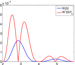
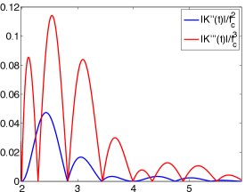
In the proof of Lemmas 2.3 and 2.4, it is necessary to find a numerical upper bound on $F_{\ell}(\Delta_{\text{min}},t)$ at $t\in\{0,0.1649\,\lambda_{c},0.4269\,\lambda_{c},0.7559\,\lambda_{c}\}$ (for the last two, we only need bounds for $\ell=0,1$). For a fixed $t$, it is easy to find the maximum of $\left|K^{\left(\ell\right)}\left(t-t_{+}\right)\right|$ where $t_{+}$ ranges over $[\Delta_{\text{min}},3\Delta_{\text{min}}]$ since we have expressions for the smooth functions $K^{(\ell)}$ (see Section B of the Appendix). For reference, these functions are plotted in Figure 6. The necessary upper bounds are gathered in Table 1.

$t/\lambda_{c}$	$F_{0}\left(1.98\lambda_{c},t\right)$	$F_{1}\left(1.98\lambda_{c},t\right)$	$F_{2}\left(1.98\lambda_{c},t\right)$	$F_{3}\left(1.98\lambda_{c},t\right)$
$0$	$6.253\;10^{-3}$	$7.639\;10^{-2}f_{c}$	$1.053\,f_{c}^{2}$	$8.078\,f_{c}^{3}$
$0.1649$	$6.279\;10^{-3}$	$7.659\;10^{-2}f_{c}$	$1.055\,f_{c}^{2}$	$18.56\,f_{c}^{3}$
$0.4269$	$8.029\;10^{-3}$	$0.3042f_{c}$
$0.7559$	$5.565\;10^{-2}$	$1.918f_{c}$

Table 1: Numerical upper bounds on $F_{\ell}(1.98\lambda_{c},t)$.

Figure 6: $\left|K^{(\ell)}\left(t\right)\right|$ for $t\in[\Delta_{\text{min}},3\Delta_{\text{min}}]$. The scaling of the $x$-axis is in units of $\lambda_{c}$.

Finally, a last fact we shall use is that $K\left(0\right)=1$ is the global maximum of $K$ and $\left|K^{\prime\prime}\left(0\right)\right|=\left|-\pi^{2}f_{c}\left(f_{c}+4\right)/3\right|$ the global maximum of $\left|K^{\prime\prime}\right|$.

2.3.1 Proof of Lemma 2.2

Set

$$\left(D_{0}\right)_{jk}=K\left(t_{j}-t_{k}\right),\quad\left(D_{1}\right)_{jk}=K^{\prime}\left(t_{j}-t_{k}\right),\quad\left(D_{2}\right)_{jk}=K^{\prime\prime}\left(t_{j}-t_{k}\right),$$

where $j$ and $k$ range from $1$ to $\left|T\right|$. With this, (2.5) and (2.6) become

$$\begin{bmatrix}D_{0}&D_{1}\\ D_{1}&D_{2}\end{bmatrix}\begin{bmatrix}\alpha\\ \beta\end{bmatrix}=\begin{bmatrix}v\\ 0\end{bmatrix}.$$

A standard linear algebra result asserts that this system is invertible if and only if $D_{2}$ and its Schur complement $D_{0}-D_{1}D_{2}^{-1}D_{1}$ are both invertible. To prove that this is the case we can use the fact that a symmetric matrix $M$ is invertible if

$$\left|\left|\text{\em I}-M\right|\right|_{\infty}<1,$$ (2.12)

where $\|A\|_{\infty}$ is the usual infinity norm of a matrix defined as $\|A\|_{\infty}=\max_{\|x\|_{\infty}=1}\|Ax\|_{\infty}=\max_{i}\sum_{j}|a_{ij}|$. This follows from $M^{-1}=(I-H)^{-1}=\sum_{k\geq 0}H^{k}$, $H=I-M$, where the series is convergent since $\left|\left|H\right|\right|_{\infty}<1$. In particular,

$$\left|\left|M^{-1}\right|\right|_{\infty}\leq\frac{1}{1-\left|\left|\text{\em I}-M\right|\right|_{\infty}}.$$ (2.13)

We also make use of the inequalities below, which follow from Lemma 2.7

$$\left|\left|\text{\em I}-D_{0}\right|\right|_{\infty} \leq F_{0}\left(\Delta_{\text{min}},0\right)\leq 6.253\;10^{-3},$$ (2.14)

$$\left|\left|D_{1}\right|\right|_{\infty} \leq F_{1}\left(\Delta_{\text{min}},0\right)\leq 7.639\;10^{-2}\;f_{c},$$ (2.15)

$$\left|\left|\left|K^{\prime\prime}\left(0\right)\right|\text{\em I}-D_{2}\right|\right|_{\infty} \leq F_{2}\left(\Delta_{\text{min}},0\right)\leq 1.053\;f_{c}^{2}\text{.}$$ (2.16)

Note that $D_{2}$ is symmetric because the second derivative of the interpolation kernel is symmetric. The bound (2.16) and the identity $K^{\prime\prime}\left(0\right)=-\pi^{2}f_{c}\left(f_{c}+4\right)/3$ give

$$\left|\left|\text{\em I}-\frac{D_{2}}{\left|K^{\prime\prime}\left(0\right)\right|}\right|\right|_{\infty}<1,$$

which implies the invertibility of $D_{2}$. The bound (2.13) then gives

$$\left|\left|D_{2}^{-1}\right|\right|_{\infty}\leq\frac{1}{\left|K^{\prime\prime}\left(0\right)\right|-\left|\left|\left|K^{\prime\prime}\left(0\right)\right|\text{\em I}-D_{2}\right|\right|_{\infty}}\leq\frac{0.4275}{f_{c}^{2}}.$$ (2.17)

Combining this with (2.14) and (2.15) yields

$$\left|\left|\text{\em I}-\left(D_{0}-D_{1}D_{2}^{-1}D_{1}\right)\right|\right|_{\infty} \leq\left|\left|\text{\em I}-D_{0}\right|\right|_{\infty}+\left|\left|D_{1}\right|\right|_{\infty}^{2}\left|\left|D_{2}^{-1}\right|\right|_{\infty}$$

$$\leq 8.747\;10^{-3}<1\text{.}$$ (2.18)

Note that the Schur complement of $D_{2}$ is symmetric because $D_{0}$ and $D_{2}$ are both symmetric whereas $D_{1}^{T}=-D_{1}$ since the derivative of the interpolation kernel is odd. This shows that the Schur complement of $D_{2}$ is invertible and, therefore, the coefficient vectors $\alpha$ and $\beta$ are well defined.

There just remains to bound the interpolation coefficients, which can be expressed as

$$\begin{bmatrix}\alpha\\ \beta\end{bmatrix}=\begin{bmatrix}\text{\em I}\\ -D_{2}^{-1}D_{1}\end{bmatrix}C^{-1}v,\quad C:=D_{0}-D_{1}D_{2}^{-1}D_{1},$$

where $C$ is the Schur complement. The relationships (2.13) and (2.18) immediately give a bound on the magnitude of the entries of $\alpha$

$$\left|\left|\alpha\right|\right|_{\infty}=\left|\left|C^{-1}v\right|\right|_{\infty}\leq\left|\left|C^{-1}\right|\right|_{\infty}\leq 1+8.824\;10^{-3}.$$

Similarly, (2.15), (2.17) and (2.18) allow to bound the entries of $\beta$:

$$\left|\left|\beta\right|\right|_{\infty} \leq\left|\left|D_{2}^{-1}D_{1}C^{-1}\right|\right|_{\infty}$$

$$\leq\left|\left|D_{2}^{-1}\right|\right|_{\infty}\left|\left|D_{1}\right|\right|_{\infty}\left|\left|C^{-1}\right|\right|_{\infty}\leq 3.294\;10^{-2}\,\lambda_{c}.$$

Finally, with $v_{1}=1$, we can use (2.18) to show that $\alpha_{1}$ is almost equal to 1. Indeed,

$$\alpha_{1}=1-\gamma_{1},\quad\gamma_{1}=[(\text{\em I}-C^{-1})v]_{1},$$

$\left|\gamma_{1}\right|\leq\left|\left|\text{\em I}-C^{-1}\right|\right|_{\infty}$, and

$$\left|\left|\text{\em I}-C^{-1}\right|\right|_{\infty}=\left|\left|C^{-1}(\text{\em I}-C)\right|\right|_{\infty}\leq\left|\left|C^{-1}\right|\right|_{\infty}\,\left|\left|\text{\em I}-C\right|\right|_{\infty}\leq 8.824\;10^{-3}.$$

This concludes the proof.

2.3.2 Proof of Lemma 2.3

We assume without loss of generality that $\tau=0$ and $q(0)=1$. By symmetry, it suffices to show the claim for $t\in(0,0.1649\,\lambda_{c}]$. Since $q^{\prime}(0)=0$, local strict concavity would imply that $\left|q\left(t\right)\right|<1$ near the origin. We begin by showing that the second derivative of $\left|q\right|$ is strictly negative in the interval $\left(0,0.1649\,\lambda_{c}\right)$. This derivative is equal to

$$\frac{\text{d}^{2}\left|q\right|}{\text{d}t^{2}}\left(t\right)=-\frac{\left(q_{R}\left(t\right)q_{R}^{\prime}\left(t\right)+q_{I}\left(t\right)q_{I}^{\prime}\left(t\right)\right)^{2}}{\left|q\left(t\right)\right|^{3}}+\frac{\left|q^{\prime}\left(t\right)\right|^{2}+q_{R}\left(t\right)q_{R}^{\prime\prime}\left(t\right)+q_{I}\left(t\right)q_{I}^{\prime\prime}\left(t\right)}{\left|q\left(t\right)\right|}\text{,}$$

where $q_{R}$ is the real part of $q$ and $q_{I}$ the imaginary part. As a result, it is sufficient to show that

$$q_{R}\left(t\right)q_{R}^{\prime\prime}\left(t\right)+\left|q^{\prime}\left(t\right)\right|^{2}+\left|q_{I}\left(t\right)\right|\left|q_{I}^{\prime\prime}\left(t\right)\right|<0\text{,}$$ (2.19)

as long as $\left|q\left(t\right)\right|$ is bounded away from zero. In order to bound the different terms in (2.19), we use the series expansions of the interpolation kernel and its derivatives around the origin to obtain the inequalities, which hold for all $t\in[-1/2,1/2]$,

$$K\left(t\right) \geq 1-\frac{\pi^{2}}{6}f_{c}\left(f_{c}+4\right)t^{2},$$ (2.20)

$$\left|K^{\prime}\left(t\right)\right| \leq\frac{\pi^{2}}{3}f_{c}\left(f_{c}+4\right)\,t,$$ (2.21)

$$K^{\prime\prime}\left(t\right) \leq-\frac{\pi^{2}}{3}f_{c}\left(f_{c}+4\right)+\frac{\pi^{4}}{6}\left(f_{c}+2\right)^{4}\,t^{2},$$ (2.22)

$$\left|K^{\prime\prime}\left(t\right)\right| \leq\frac{\pi^{2}}{3}f_{c}\left(f_{c}+4\right),$$ (2.23)

$$\left|K^{\prime\prime\prime}\left(t\right)\right| \leq\frac{\pi^{4}}{3}\left(f_{c}+2\right)^{4}\,t.$$ (2.24)

The lower bounds are decreasing in $t$, while the upper bounds are increasing in $t$, so we can evaluate them at $0.1649\,\lambda_{c}$ to establish that for all $t\in[0,0.1649\,\lambda_{c}]$,

$$K\left(t\right) \geq 0.9539, \qquad K^{\prime\prime}\left(t\right) \leq-2.923\,f_{c}^{2},$$ (2.25)

$$\left|K^{\prime}\left(t\right)\right| \leq 0.5595\,f_{c}, \qquad\left|K^{\prime\prime}\left(t\right)\right| \leq 3.393\,f_{c}^{2}, \qquad\left|K^{\prime\prime\prime}\left(t\right)\right| \leq 5.697\,f_{c}^{3}.$$

We combine this with Lemmas 2.7 and 2.2 to control the different terms in (2.19) and begin with $q_{R}\left(t\right)$. Here,

$$q_{R}\left(t\right) =\sum_{t_{j}\in T}\text{Re}\left(\alpha_{j}\right)K\left(t-t_{j}\right)+\text{Re}\left(\beta_{j}\right)K^{\prime}\left(t-t_{j}\right)$$

$$\geq\text{Re}\left(\alpha_{1}\right)K\left(t\right)-\left|\left|\alpha\right|\right|_{\infty}\sum_{t_{j}\in T\setminus\left\{0\right\}}\left|K\left(t-t_{j}\right)\right|-\left|\left|\beta\right|\right|_{\infty}\sum_{t_{j}\in T}\left|K^{\prime}\left(t-t_{j}\right)\right|$$

$$\geq\text{Re}\left(\alpha_{1}\right)K\left(t\right)-\alpha^{\infty}F_{0}\left(\Delta,t\right)-\beta^{\infty}\left(\left|K^{\prime}\left(t\right)\right|+F_{1}\left(\Delta,t\right)\right)$$

$$\geq\text{Re}\left(\alpha_{1}\right)K\left(t\right)-\alpha^{\infty}F_{0}\left(\Delta_{\text{min}},t\right)-\beta^{\infty}\left(\left|K^{\prime}\left(t\right)\right|+F_{1}\left(\Delta_{\text{min}},t\right)\right)\geq 0.9182\text{.}$$ (2.26)

The third inequality follows from the monotonicity of $F_{\ell}$ in $\Delta$, and the last from (2.25) together with the monotonicity of $F_{1}\left(\Delta_{\text{min}},t\right)$ in $t$, see Lemma 2.7, so that we can plug in $t=0.1649\,\lambda_{c}$. Observe that this shows that $q$ is bounded away from zero since $\left|q\left(t\right)\right|\geq q_{R}\left(t\right)\geq 0.9198$. Very similar computations yield

$$\left|q_{I}\left(t\right)\right| =\left|\sum_{t_{j}\in T}\text{Im}\left(\alpha_{j}\right)K\left(t-t_{j}\right)+\text{Im}\left(\beta_{j}\right)K^{\prime}\left(t-t_{j}\right)\right|$$

$$\leq\left|\text{Im}\left(\alpha_{1}\right)\right|+\left|\left|\alpha\right|\right|_{\infty}\sum_{t_{j}\in T\setminus\left\{0\right\}}\left|K\left(t-t_{j}\right)\right|+\left|\left|\beta\right|\right|_{\infty}\sum_{t_{j}\in T}\left|K^{\prime}\left(t-t_{j}\right)\right|$$

$$\leq\left|\text{Im}\left(\alpha_{1}\right)\right|+\alpha^{\infty}F_{0}\left(\Delta_{\text{min}},t\right)+\beta^{\infty}\left(\left|K^{\prime}\left(t\right)\right|+F_{1}\left(\Delta_{\text{min}},t\right)\right)\leq 3.611\;10^{-2}$$

and

$$q_{R}^{\prime\prime}\left(t\right) =\sum_{t_{j}\in T}\text{Re}\left(\alpha_{j}\right)K^{\prime\prime}\left(t-t_{j}\right)+\sum_{t_{j}\in T}\text{Re}\left(\beta_{j}\right)K^{\prime\prime\prime}\left(t-t_{j}\right)$$

$$\leq\text{Re}\left(\alpha_{1}\right)K^{\prime\prime}\left(t\right)+\left|\left|\alpha\right|\right|_{\infty}\sum_{t_{j}\in T\setminus\left\{0\right\}}\left|K^{\prime\prime}\left(t-t_{j}\right)\right|+\left|\left|\beta\right|\right|_{\infty}\sum_{t_{j}\in T}\left|K^{\prime\prime\prime}\left(t-t_{j}\right)\right|$$

$$\leq\text{Re}\left(\alpha_{1}\right)K^{\prime\prime}\left(t\right)+\alpha^{\infty}F_{2}\left(\Delta_{\text{min}},t\right)+\beta^{\infty}\left(\left|K^{\prime\prime\prime}\left(t\right)\right|+F_{3}\left(\Delta_{\text{min}},t\right)\right)\leq-1.034\,f_{c}^{2}.$$ (2.27)

Similarly,

$$\left|q_{I}^{\prime\prime}\left(t\right)\right| =\left|\sum_{t_{j}\in T}\text{Im}\left(\alpha_{j}\right)K^{\prime\prime}\left(t-t_{j}\right)+\sum_{t_{j}\in T}\text{Im}\left(\beta_{j}\right)K^{\prime\prime\prime}\left(t-t_{j}\right)\right|$$

$$\leq\text{Im}\left(\alpha_{1}\right)\left|K^{\prime\prime}\left(t\right)\right|+\left|\left|\alpha\right|\right|_{\infty}\sum_{t_{j}\in T\setminus\left\{0\right\}}\left|K^{\prime\prime}\left(t-t_{j}\right)\right|+\left|\left|\beta\right|\right|_{\infty}\sum_{t_{j}\in T}\left|K^{\prime\prime\prime}\left(t-t_{j}\right)\right|$$

$$\leq\text{Im}\left(\alpha_{1}\right)\left|K^{\prime\prime}\left(t\right)\right|+\alpha^{\infty}F_{2}\left(\Delta_{\text{min}},t\right)+\beta^{\infty}\left(\left|K^{\prime\prime\prime}\left(t\right)\right|+F_{3}\left(\Delta_{\text{min}},t\right)\right)\leq 1.893\,f_{c}^{2}$$

and

$$\left|q^{\prime}\left(t\right)\right| =\left|\sum_{t_{j}\in T}\alpha_{j}K^{\prime}\left(t-t_{j}\right)+\beta_{j}K^{\prime\prime}\left(t-t_{j}\right)\right|$$

$$\leq\left|\left|\alpha\right|\right|_{\infty}\sum_{t_{j}\in T}\left|K^{\prime}\left(t-t_{j}\right)\right|+\left|\left|\beta\right|\right|_{\infty}\sum_{t_{j}\in T}\left|K^{\prime\prime}\left(t-t_{j}\right)\right|$$

$$\leq\alpha^{\infty}\left|K^{\prime}\left(t\right)\right|+\alpha^{\infty}F_{1}\left(\Delta_{\text{min}},t\right)+\beta^{\infty}\left(\left|K^{\prime\prime}\left(t\right)\right|+F_{2}\left(\Delta_{\text{min}},t\right)\right)\leq 0.7882\,f_{c}\text{.}$$

These bounds allow us to conclude that $|q|^{\prime\prime}$ is negative on $[0,0.1649\lambda_{c}]$ since

$$q_{R}\left(t\right)q_{R}^{\prime\prime}\left(t\right)+\left|q^{\prime}\left(t\right)\right|^{2}+\left|q_{I}\left(t\right)\right|\left|q_{I}^{\prime\prime}\left(t\right)\right|\leq-9.291\;10^{-2}f_{c}^{2}<0.$$

This completes the proof.

2.3.3 Proof of Lemma 2.4

As before, we assume without loss of generality that $\tau=0$ and $q(0)=1$. We use Lemma 2.7 again to bound the absolute value of the dual polynomial on $[0.1649\lambda_{c},\Delta/2]$ and write

$$\left|q\left(t\right)\right| =\Bigl{|}\sum_{t_{j}\in T}\alpha_{j}K\left(t-t_{j}\right)+\beta_{j}K^{\prime}\left(t-t_{j}\right)\Bigr{|}$$

$$\leq\left|\left|\alpha\right|\right|_{\infty}\Bigl{[}\left|K\left(t\right)\right|+\sum_{t_{j}\in T\setminus\left\{0\right\}}\left|K\left(t-t_{j}\right)\right|\Bigr{]}+\left|\left|\beta\right|\right|_{\infty}\Bigl{[}\left|K^{\prime}\left(t\right)\right|+\sum_{t_{j}\in T\setminus\left\{0\right\}}\left|K^{\prime}\left(t-t_{j}\right)\right|\Bigr{]}$$

$$\leq\alpha^{\infty}\left|K\left(t\right)\right|+\alpha^{\infty}F_{0}\left(\Delta_{\text{min}},t\right)+\beta^{\infty}\left|K^{\prime}\left(t\right)\right|+\beta^{\infty}F_{1}\left(\Delta_{\text{min}},t\right).$$ (2.28)

Note that we are assuming adversarial sign patterns and as a result we are unable to exploit cancellations in the coefficient vectors $\alpha$ and $\beta$. To control $|K(t)|$ and $|K^{\prime}(t)|$ between $0.1649\,\lambda_{c}$ and $0.7559\,\lambda_{c}$, we use series expansions around the origin which give

$$K\left(t\right) \leq 1-\frac{\pi^{2}f_{c}\left(f_{c}+4\right)t^{2}}{6}+\frac{\pi^{4}\left(f_{c}+2\right)^{4}t^{4}}{72}$$ (2.29)

$$\left|K^{\prime}\left(t\right)\right| \leq\frac{\pi^{2}f_{c}\left(f_{c}+4\right)t}{3},$$

for all $t\in[-1/2,1/2]$. Put

$$L_{1}\left(t\right)=\alpha^{\infty}\Bigl{[}1-\frac{\pi^{2}f_{c}\left(f_{c}+4\right)t^{2}}{6}+\frac{\pi^{4}\left(f_{c}+2\right)^{4}t^{4}}{72}\Bigr{]}+\beta^{\infty}\frac{\pi^{2}f_{c}\left(f_{c}+4\right)t}{3},$$

with derivative equal to

$$L_{1}^{\prime}\left(t\right)=-\alpha^{\infty}\Bigl{[}\frac{\pi^{2}f_{c}\left(f_{c}+4\right)t}{3}-\frac{\pi^{4}\left(f_{c}+2\right)^{4}t^{3}}{18}\Bigr{]}+\beta^{\infty}\frac{\pi^{2}f_{c}\left(f_{c}+4\right)}{3}\text{.}$$

This derivative is strictly negative between $0.1649\,\lambda_{c}$ and $0.7559\,\lambda_{c}$, which implies that $L_{1}\left(t\right)$ is decreasing in this interval. Put

$$L_{2}\left(t\right)=\alpha^{\infty}F_{0}\left(\Delta_{\text{min}},t\right)+\beta^{\infty}F_{1}\left(\Delta_{\text{min}},t\right).$$

By Lemma 2.7, this function is increasing. With (2.28), this gives the crude bound

$$\left|q\left(t\right)\right|\leq L_{1}\left(t\right)+L_{2}\left(t\right)\leq L_{1}\left(t_{1}\right)+L_{2}\left(t_{2}\right)\quad\text{for all }t\in[t_{1},t_{2}].$$ (2.30)

Table 2 shows that taking $\left\{t_{1},t_{2}\right\}=\left\{0.1649\,\lambda_{c},0.4269\,\lambda_{c}\right\}$ and then $\left\{t_{1},t_{2}\right\}=\left\{0.4269\,\lambda_{c},0.7559\,\lambda_{c}\right\}$ proves that $\left|q(t)\right|<1$ on $[0.1649\lambda_{c},0.7559\lambda_{c}]$. For $0.7559\lambda_{c}\leq t\leq\Delta/2$, we apply Lemma 2.6 and obtain

$$|q(t)| \leq\alpha^{\infty}\Bigl{[}B_{0}\left(t\right)+B_{0}\left(\Delta-t\right)+\sum_{j=1}^{\infty}B_{0}\left(j\Delta_{\text{min}}+\Delta-t\right)+\sum_{j=1}^{\infty}B_{0}\left(j\Delta_{\text{min}}+t\right)\Bigr{]}$$

$$\qquad\qquad+\beta^{\infty}\Bigl{[}B_{1}\left(t\right)+B_{1}\left(\Delta-t\right)+\sum_{j=1}^{\infty}B_{1}\left(j\Delta_{\text{min}}+\Delta-t\right)+\sum_{j=1}^{\infty}B_{1}\left(j\Delta_{\text{min}}+t\right)\Bigr{]}$$

$$\leq\alpha^{\infty}\Bigl{[}B_{0}\left(0.7559\lambda_{c}\right)+\sum_{j=1}^{\infty}B_{0}\left(j\Delta_{\text{min}}-0.7559\lambda_{c}\right)+\sum_{j=1}^{\infty}B_{0}\left(j\Delta_{\text{min}}+0.7559\lambda_{c}\right)\Bigr{]}$$

$$\qquad\qquad+\beta^{\infty}\Bigl{[}B_{1}\left(0.7559\lambda_{c}\right)+\sum_{j=1}^{\infty}B_{1}\left(j\Delta_{\text{min}}-0.7559\lambda_{c}\right)+\sum_{j=1}^{\infty}B_{1}\left(j\Delta_{\text{min}}+0.7559\lambda_{c}\right)\Bigr{]}$$

$$\leq 0.758;$$

here, the second step follows from the monotonicity of $B_{0}$ and $B_{1}$. Finally, for $\Delta/2\leq t\leq t_{+}/2$, this last inequality applies as well. This completes the proof.

$t_{1}/\lambda_{c}$	$t_{2}/\lambda_{c}$	$L_{1}\left(t_{1}\right)$	$L_{2}\left(t_{2}\right)$
$0.1649$	$0.4269$	$0.9818$	$1.812\,10^{-2}$
$0.4269$	$0.7559$	$0.7929$	$0.2068$

Table 2: Numerical quantities used in (2.30).

2.4 Proof of Lemma 2.5

Replacing $\Delta=1.98\,\lambda_{c}$ by $\Delta=2.5\,\lambda_{c}$ and going through exactly the same calculations as in Sections 2.3.1 and 2.3.2 yields that for any $t$ obeying $0\leq\left|t-\tau\right|\leq 0.1649\,\lambda_{c}$,

$$\frac{\text{d}^{2}\left|q\right|}{\text{d}t^{2}}\left(t\right)\leq-0.6706\,f_{c}^{2}.$$

For reference, we have computed in Table 3 numerical upper bounds on $F_{\ell}(2.5\lambda_{c},t)$ at $t=\{0,0.1649\,\lambda\}$. Since $|q(0)|=1$ and $q^{\prime}(0)=0$, it follows that

$$\left|q\left(t\right)\right|\leq\left|q\left(0\right)\right|-\frac{1}{2}\,{0.6706\,f_{c}^{2}}t^{2}.$$ (2.31)

At a distance of $0.1649\,\lambda_{c}$, the right-hand side is equal to $0.9909$. The calculations in Section 2.3.3 with $\Delta=2.5\,\lambda_{c}$ imply that the magnitude of $q(t)$ at locations at least $0.1649\,\lambda_{c}$ away from an element of $T$ is bounded by $0.9843$. This concludes the proof.

$t/\lambda_{c}$	$F_{0}\left(2.5\lambda_{c},t\right)$	$F_{1}\left(2.5\lambda_{c},t\right)$	$F_{2}\left(2.5\lambda_{c},t\right)$	$F_{3}\left(2.5\lambda_{c},t\right)$
$0$	$5.175\;10^{-3}$	$6.839\;10^{-2}f_{c}$	$0.8946\,f_{c}^{2}$	$7.644\,f_{c}^{3}$
$0.1649$	$5.182\;10^{-3}$	$6.849\;10^{-2}f_{c}$	$0.9459\,f_{c}^{2}$	$7.647\,f_{c}^{3}$

Table 3: Numerical upper bounds on $F_{\ell}(2.5\lambda_{c},t)$.

2.5 Improvement for real-valued signals

The proof for real-valued signals is almost the same as the one we have discussed for complex-valued signals—only simpler. The only modification to Lemmas 2.2 and 2.4 is that the minimum distance is reduced to $1.87\,\lambda_{c}$, and that the bound in Lemma 2.4 is shown to hold starting at $0.17\,\lambda_{c}$ instead of $0.1649\,\lambda_{c}$. For reference, we provide upper bounds on $F_{\ell}(1.87\lambda_{c},t)$ at $t\in\{0,0.17\,\lambda_{c}\}$ in Table 4. As to Lemma 2.3, the only difference is that to bound $\left|q\right|$ between the origin and $0.17\,\lambda_{c}$, it is sufficient to show that the second derivative of $q$ is negative and make sure that $q>-1$. Computing (2.27) for $\Delta=1.87\lambda_{c}$ for $t\in[0,0.17\,\lambda_{c}]$, we obtain $q^{\prime\prime}<-0.1181$. Finally, (2.26) yields $q>0.9113$ in $[0,0.17\,\lambda_{c}]$.

$t/\lambda_{c}$	$F_{0}\left(1.87\lambda_{c},t\right)$	$F_{1}\left(1.87\lambda_{c},t\right)$	$F_{2}\left(1.87\lambda_{c},t\right)$	$F_{3}\left(1.87\lambda_{c},t\right)$
$0$	$6.708\;10^{-3}$	$7.978\;10^{-2}f_{c}$	$1.078\,f_{c}^{2}$	$16.01\,f_{c}^{3}$
$0.17$	$6.747\;10^{-3}$	$0.1053f_{c}$	$1.081\,f_{c}^{2}$	$41.74\,f_{c}^{3}$

Table 4: Numerical upper bounds on $F_{\ell}(1.87\lambda_{c},t)$.

3 Stability

This section proves Theorem 1.5 and we begin by establishing a strong form of the null-space property. In the remainder of the paper $P_{T}$ is the orthogonal projector onto the linear space of vectors supported on $T$, namely, $(P_{T}x)_{i}=x_{i}$ if $i\in T$ and is zero otherwise.

Lemma 3.1

Under the assumptions of Theorem 1.5, any vector $h$ such that $F_{n}h=0$ obeys

$$\left|\left|P_{T}h\right|\right|_{1}\leq\rho\left|\left|P_{T^{c}}h\right|\right|_{1},$$ (3.1)

for some numerical constant $\rho$ obeying $0<\rho<1$. This constant is of the form $1-\rho=\alpha/\text{\em SRF}^{2}$ for some positive $\alpha>0$. If $\text{SRF}\geq 3.03$, we can take $\alpha=0.0883$.

Proof Let $P_{T}h_{t}=\left|P_{T}h_{t}\right|e^{i\phi_{t}}$ be the polar decomposition of $P_{T}h$, and consider the low-frequency polynomial $q(t)$ in Proposition 2.1 interpolating $v_{t}=e^{-i\phi_{t}}$. We shall abuse notations and set $q=\{q_{t}\}_{t=0}^{N-1}$ where $q_{t}=q(t/N)$. For $t\notin T$, $|q(t/N)|=|q_{t}|\leq\rho<1$. By construction $q=P_{n}q$, and thus $\langle q,h\rangle=\langle q,P_{n}h\rangle=0$. Also,

$$\langle P_{T}q,P_{T}h\rangle=\|P_{T}h\|_{1}.$$

The conclusion follows from

$$0=\langle q,h\rangle=\langle P_{T}q,P_{T}h\rangle+\langle P_{T^{c}}q,P_{T^{c}}h\rangle\geq\|P_{T}h\|_{1}-\|P_{T^{c}}q\|_{\infty}\|P_{T^{c}}h\|_{1}\geq\|P_{T}h\|_{1}-\rho\|P_{T^{c}}h\|_{1}.$$

For the numerical constant, we use Lemma 2.5 which says that if $0\in T$ and $1/N\leq 0.1649\lambda_{c}$, which is about the same as $1/\text{SRF}\approx 2f_{c}/N\leq 2\times 0.1649$ or $\text{SRF}>3.03$, we have

$$|q(1/N)|\leq 1-0.3533\,(f_{c}/N)^{2}\approx 1-0.0883/\text{SRF}^{2}=\rho.$$

This applies directly to any other $t$ such that $\min_{\tau\in T}\left|t-\tau\right|=1$. Also, for all $t$ at distance at least 2 from $T$, Lemma 2.5 implies that $|q(t/N)|\leq\rho$. This completes the proof.  

3.1 Proof of Theorem 1.5

The proof is a fairly simple consequence of Lemma 3.1. Set $h=\hat{x}-x$ and decompose the error into its low- and high-pass components

$$h_{L}=P_{n}h,\quad h_{H}=h-h_{L}.$$

The high-frequency part is in the null space of $P_{n}$ and (3.1) gives

$$\left|\left|P_{T}h_{H}\right|\right|_{1}\leq\rho\left|\left|P_{T^{c}}h_{H}\right|\right|_{1}.$$ (3.2)

For the low-frequency component we have

$$\|h_{L}\|_{1}=\|P_{n}(\hat{x}-x)\|_{1}\leq\|P_{n}\hat{x}-s\|_{1}+\|s-P_{n}x\|_{1}\leq 2\delta.$$ (3.3)

To bound $\|P_{T^{c}}h_{H}\|_{1}$, we exploit the fact that $\hat{x}$ has minimum $\ell_{1}$ norm. We have

$$\left|\left|x\right|\right|_{1}\geq\left|\left|x+h\right|\right|_{1} \geq\left|\left|x+h_{H}\right|\right|_{1}-\|h_{L}\|_{1}$$

$$\geq\|x\|_{1}-\left|\left|P_{T}h_{H}\right|\right|_{1}+\left|\left|P_{T^{c}}h_{H}\right|\right|_{1}-\|h_{L}\|_{1}$$

$$\geq\|x\|_{1}+(1-\rho)\left|\left|P_{T^{c}}h_{H}\right|\right|_{1}-\|h_{L}\|_{1},$$

where the last inequality follows from (3.2). Hence,

$$\left|\left|P_{T^{c}}h_{H}\right|\right|_{1}\leq\frac{1}{1-\rho}\|h_{L}\|_{1}\quad\Rightarrow\quad\|h_{H}\|_{1}\leq\frac{1+\rho}{1-\rho}\,\|h_{L}\|_{1}.$$

To conclude,

$$\|h\|_{1}\leq\|h_{L}\|_{1}+\|h_{H}\|_{1}\leq\frac{2}{1-\rho}\|h_{L}\|_{1}\leq\frac{4\delta}{1-\rho},$$

where the last inequality follows from (3.3).

Since from Lemma 3.1, we have $1-\rho=\alpha/\text{SRF}^{2}$ for some numerical constant $\alpha$, the upper bound is of the form $4\alpha^{-1}\,\text{SRF}^{2}\,\delta$. For $\Delta(T)\geq 2.5\lambda_{c}$, we have $\alpha^{-1}\approx 11.235$.

3.2 Sparsity is not enough

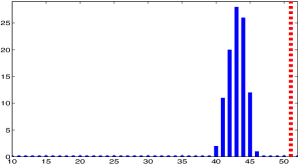
Consider the vector space $\mathbb{C}^{48}$ of sparse signals of length $N=4096$ supported on a certain interval of length 48. Figure 7 shows the eigenvalues of the low-pass filter $P_{n}=\frac{1}{N}F_{n}F_{n}^{*}$ acting on $\mathbb{C}^{48}$ for different values of the super-resolution factor. For $\text{SRF}=4$, there exists a subspace of dimension 24 such that any unit-normed signal ($\|x\|_{2}=1$) belonging to it obeys

$$\|P_{n}x\|_{2}\leq 2.52\;10^{-15}\quad\Leftrightarrow\quad\frac{1}{\sqrt{N}}\|F_{n}x\|_{2}\leq 5.02\;10^{-8}.$$

For $\text{SRF}=16$ this is true of a subspace of dimension 36, two thirds of the total dimension. Such signals can be completely canceled out by perturbations of norm $5.02\;10^{-8}$, so that even at signal-to-noise ratios (SNR) of more than 145 dB, recovery is impossible by any method whatsoever.

Figure 7: (a) Eigenvalues of $P_{n}$ acting on signals supported on a contiguous interval of length $48$ for super-resolution factors of 2, 4, 8 and 16 and a signal length of $4096$. (b) Singular values of $\frac{1}{\sqrt{N}}F_{n}$ on a logarithmic scale. (c) Same as (b) but on a linear scale. Due to limited numerical precision (machine precision), the smallest singular values, marked with circular dots on the graphs, are of course not computed accurately.

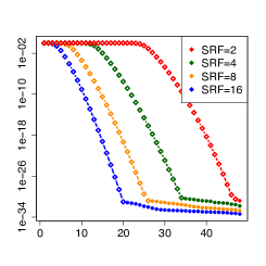
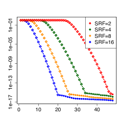
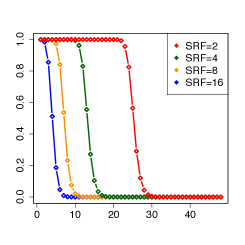
Interestingly, the sharp transition shown in Figure 7 between the first singular values almost equal to one and the others, which rapidly decay to zero, can be characterized asymptotically by using the work of Slepian on prolate spheroidal sequences [36]. Introduce the operator $\mathcal{T}_{k}$, which sets the value of an infinite sequence to zero on the complement of an interval $T$ of length $k$. With the notation of Section 1.7, the eigenvectors of the operator $\mathcal{P}_{W}\mathcal{T}_{k}$ are the discrete prolate spheroidal sequences $\{s_{j}\}_{j=1}^{k}$ introduced in [36],

$$\mathcal{P}_{W}\mathcal{T}_{k}s_{j}=\lambda_{j}s_{j},\quad 1>\lambda_{1}\geq\lambda_{2}\geq\ldots\geq\lambda_{k}>0.$$ (3.4)

Set $v_{j}=\mathcal{T}_{k}s_{j}/\sqrt{\lambda_{j}}$, then by (3.4), it is not hard to see that

$$\mathcal{T}_{k}\mathcal{P}_{W}v_{j}=\lambda_{j}v_{j},\qquad\left|\left|v_{j}\right|\right|_{2}=1.$$

In fact, the $v_{j}$’s are also orthogonal to each other [36], and so they form an orthonormal basis of $\mathbb{C}^{k}$ (which can represent any sparse vector supported on $T$). For values of $j$ near $k$, the value of $\lambda_{j}$ is about

$$A_{j}e^{-\gamma\left(k+1\right)},\quad\quad A_{j}=\frac{\sqrt{\pi}2^{\frac{14\left(k-j\right)+9}{4}}\alpha^{\frac{2\left(k-j\right)+1}{4}}\left(k+1\right)^{k-j+0.5}}{\left(k-j\right)!\left(2-\alpha\right)^{k-j+0.5}},$$

where

$$\alpha=1+\cos{2\pi W},\quad\gamma=\log\left(1+\frac{2\sqrt{\alpha}}{\sqrt{2}-\sqrt{\alpha}}\right).$$

Therefore, for a fixed value of $\text{SRF}=1/2W$, and $k\geq 20$, the small eigenvalues are equal to zero for all practical purposes. In particular, for $\text{SRF}=4$ and $\text{SRF}=1.05$ we obtain (1.17) and (1.19) in Section 1.7 respectively. Additionally, a Taylor series expansion of $\gamma$ for large values of SRF yields (1.20).

Since $\|\mathcal{P}_{W}v_{j}\|_{L_{2}}=\sqrt{\lambda_{j}}$, the bound on $\lambda_{j}$ for $j$ near $k$ directly implies that some sparse signals are essentially zeroed out, even for small super-resolution factors. However, Figure 7 suggests an even stronger statement: as the super-resolution factor increases not only some, but most signals supported on $T$ seem to be almost completely suppressed by the low pass filtering. Slepian provides an asymptotic characterization for this phenomenon. Indeed, just about the first $2kW$ eigenvalues of $\mathcal{P}_{W}\mathcal{T}_{k}$ cluster near one, whereas the rest decay abruptly towards zero. To be concrete, for any $\epsilon>0$ and $j\geq 2kW\left(1+\epsilon\right)$, there exist positive constants $C_{0}$, and $\gamma_{0}$ (depending on $\epsilon$ and $W$) such that

$$\lambda_{j}\leq C_{0}e^{-\gamma_{0}k}.$$

This holds for all $k\geq k_{0}$, where $k_{0}$ is some fixed integer. This implies that for any interval $T$ of length $k$, there exists a subspace of signals supported on $T$ with dimension asymptotically equal to $\left(1-1/\text{SRF}\right)k$, which is obliterated by the measurement process. This has two interesting consequences. First, even if the super-resolution factor is just barely above one, asymptotically there will always exist an irretrievable vector supported on $T$. Second, if the super-resolution factor is two or more, most of the information encoded in clustered sparse signals is lost. Consider for instance a random sparse vector $x$ supported on $T$ with i.i.d. entries. Its projection onto a fixed subspace of dimension about $\left(1-1/\text{SRF}\right)k$ (corresponding to the negligible eigenvalues) contains most of the energy of the signal with high probability. However, this component is practically destroyed by low-pass filtering. Hence, super-resolving almost any tightly clustered sparse signal in the presence of noise is hopeless. This justifies the need for a minimum separation between nonzero components.

4 Minimization via semidefinite programming

At first sight, finding the solution to the total-variation norm problem (1.4) might seem quite challenging, as it requires solving an optimization problem over an infinite dimensional space. It is of course possible to approximate the solution by discretizing the support of the signal, but this could lead to an increase in complexity if the discretization step is reduced to improve precision. Another possibility is to try approximating the solution by estimating the support of the signal in an iterative fashion [5]. Here, we take a different route and show that (1.4) can be cast as a semidefinite program with just $\left(n+1\right)^{2}/2$ variables, and that highly accurate solutions can be found rather easily. This formulation is similar to that in [3] which concerns a related infinite dimensional convex program. Our exposition is less formal here than in the rest of the paper.

The convex program dual to (1.4) is

$$\max_{c}\;\operatorname{Re}\langle y,c\rangle\quad\text{subject to}\quad\left|\left|\mathcal{F}_{n}^{\ast}\,c\right|\right|_{\infty}\leq 1;$$ (4.1)

the constraint says that the trigonometric polynomial $(\mathcal{F}_{n}^{\ast}\,c)(t)=\sum_{|k|\leq f_{c}}c_{k}e^{i2\pi kt}$ has a modulus uniformly bounded by $1$ over the interval $[0,1]$. The interior of the feasible set contains the origin and is consequently non empty, so that strong duality holds by a generalized Slater condition [33]. The cost function involves a finite vector of dimension $n$, but the problem is still infinite dimensional due to the constraints. A corollary to Theorem 4.24 in [17] allows to express this constraint as the intersection between the cone of positive semidefinite matrices $\{X:X\succeq 0\}$ and an affine hyperplane.

Corollary 4.1

A causal trigonometric polynomial $\sum_{k=0}^{n-1}c_{k}e^{i2\pi kt}$ with $c\in\mathbb{C}^{n}$ is bounded by one in magnitude if and only if there exists a Hermitian matrix $Q\in\mathbb{C}^{n\times n}$ obeying

$$\begin{bmatrix}Q&c\\ c^{\ast}&1\end{bmatrix}\succeq 0,\qquad\sum_{i=1}^{n-j}Q_{i,i+j}=\begin{cases}1,&j=0,\\ 0,&j=1,2,\ldots,n-1.\end{cases}$$ (4.2)

To see one direction, note that the positive semidefiniteness constraint is equivalent to $Q-cc^{\ast}\succeq 0$. Hence, $z^{\ast}Qz\geq\left|c^{\ast}z\right|^{2}$ for all $z\in\mathbb{C}^{n}$. Fix $t\in[0,1]$ and set $z_{k}=e^{i2\pi kt}$. The equality constraints in (4.2) give $z^{\ast}Qz=1$ and $\left|c^{\ast}z\right|^{2}=|(\mathcal{F}_{n}^{*}c)(t)|^{2}$ so we obtain the desired inequality constraint on the magnitude of the trigonometric polynomial $\sum_{k=0}^{n-1}c_{k}e^{i2\pi kt}$.

Returning to (4.1), the polynomial $e^{i2\pi f_{c}t}\,(\mathcal{F}_{n}^{\ast}\,c)(t)$ is causal and has the same magnitude as $(\mathcal{F}_{n}^{\ast}\,c)(t)$. Hence, the dual problem is equivalent to

$$\max_{c,Q}\;\operatorname{Re}\langle y,c\rangle\quad\text{subject to}\quad\text{\eqref{eq:sdp-charact}}.$$ (4.3)

To be complete, the decision variables are an Hermitian matrix $Q\in\mathbb{C}^{n\times n}$ and a vector of coefficients $c\in\mathbb{C}^{n}$. The finite dimensional semidefinite program can be solved by off-the-shelf convex programming software.

Figure 8: The sign of a real atomic measure $x$ is plotted in red. The trigonometric polynomial $\mathcal{F}_{n}^{\ast}c$ where $c$ is a solution to the dual problem (4.3) is plotted in blue. Note that $\mathcal{F}_{n}^{\ast}c$ interpolates the sign of $x$. Here, $f_{c}=50$ so that we have $n=101$ low-frequency coefficients.

The careful reader will observe that we have just shown how to compute the optimal value of (1.4), but not how we could obtain a solution. To find a primal solution, we abuse notation by letting $c$ be the solution to (4.3) and consider the trigonometric polynomial

$$p_{2n-2}(e^{i2\pi t})=1-\left|(\mathcal{F}_{n}^{\ast}c)(t)\right|^{2}=1-\sum_{k=-2f_{c}}^{2f_{c}}u_{k}e^{i2\pi kt},\qquad u_{k}=\sum_{j}c_{j}\bar{c}_{j-k}.$$ (4.4)

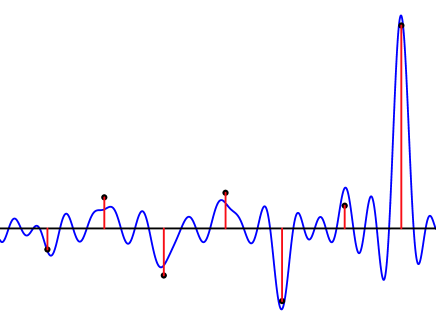
Note that $z^{2f_{c}}p_{2n-2}(z)$, where $z\in\mathbb{C}$, is a polynomial of degree $4f_{c}=2(n-1)$ with the same roots as $p_{2n-2}(z)$—besides the trivial root $z=0$. Hence, $p_{2n-2}(e^{i2\pi t})$ has at most $2n-2$ roots. By construction $p_{2n-2}(e^{i2\pi t})$ is a real-valued and nonnegative trigonometric polynomial; in particular, it cannot have single roots on the unit circle since the existence of single roots would imply that $p_{2n-2}(e^{i2\pi t})$ takes on negative values. Therefore, $p_{2n-2}(e^{i2\pi t})$ is either equal to zero everywhere or has at most $n-1$ roots on the unit circle. By strong duality, any solution $\hat{x}$ to (1.4) obeys

$$\operatorname{Re}\langle y,c\rangle=\operatorname{Re}\langle\mathcal{F}_{n}\,\hat{x},c\rangle=\operatorname{Re}\langle\hat{x},\mathcal{F}_{n}^{\ast}\,c\rangle=\operatorname{Re}\left[\int_{0}^{1}\overline{(\mathcal{F}_{n}^{\ast}c)\left(t\right)}\,\hat{x}(\text{d}t)\right]=\left|\left|\hat{x}\right|\right|_{\text{TV}},$$

which implies that the trigonometric polynomial $\mathcal{F}_{n}^{\ast}c$ is exactly equal to the sign of $\hat{x}$ when $\hat{x}$ is not vanishing. This is illustrated in Figure 8. Thus, to recover the support of the solution to the primal problem, we must simply locate the roots of $p_{2n-2}$ on the unit circle, for instance by computing the eigenvalues of its companion matrix [31]. As shown in Table 5, this scheme allows to recover the support with very high precision. Having obtained the estimate for the support $\hat{T}$, the amplitudes of the signal can be reconstructed by solving the system of equations $\sum_{t\in\hat{T}}e^{-i2\pi kt}a_{t}=y_{k}$, $\left|k\right|\leq f_{c}$, using the method of least squares. There is a unique solution as we have at most $n-1$ columns which are linearly independent since one can add columns to form a Vandermonde system.Figure 9 illustrates the accuracy of this procedure; a Matlab script reproducing this example is available at http://www-stat.stanford.edu/~candes/superres_sdp.m.

$f_{c}$	25	50	75	100
Average error	$6.66\,10^{-9}$	$1.70\,10^{-9}$	$5.58\,10^{-10}$	$2.96\,10^{-10}$
Maximum error	$1.83\,10^{-7}$	$8.14\,10^{-8}$	$2.55\,10^{-8}$	$2.31\,10^{-8}$

Table 5: Numerical recovery of the support of a sparse signal obtained by solving (4.3) via CVX [21]. For each value of the cut-off frequency $f_{c}$, 100 signals were generated with random complex amplitudes situated at approximately $f_{c}/4$ random locations in the unit interval separated by at least $2/f_{c}$. The table shows the errors in estimating the support locations.

Figure 9: There are 21 spikes situated at arbitrary locations separated by at least $2\lambda_{c}$ and we observe 101 low-frequency coefficients ($f_{c}=50$). In the plot, seven of the original spikes (black dots) are shown along with the corresponding low resolution data (blue line) and the estimated signal (red line).

Figure 10: The trigonometric polynomial $p_{2n-2}(e^{i2\pi t})$ with random data $y\in\mathbb{C}^{21}$ ($n=21$ and $f_{c}=10$) with i.i.d. complex Gaussian entries. The polynomial has 16 roots.

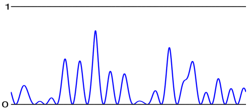
In summary, in the usual case when $p_{2n-2}$ has less than $n$ roots on the unit circle, we have explained how to retrieve the minimum total-variation norm solution. It remains to address the situation in which $p_{2n-2}$ vanishes everywhere. In principle, this could happen even if a primal solution to (1.4) is an atomic measure supported on a set $T$ obeying $|T|<n$. For example, let $x$ be a positive measure satisfying the conditions of Theorem 1.2, which implies that it is the unique solution to (1.4). Consider a vector $c\in\mathbb{C}^{n}$ such that $(\mathcal{F}_{n}^{\ast}c)(t)=1$; i. e., the trigonometric polynomial is constant. Then

$$\operatorname{Re}\langle y,c\rangle=\operatorname{Re}\langle\mathcal{F}_{n}\,x,c\rangle=\operatorname{Re}\langle x,\mathcal{F}_{n}^{\ast}\,c\rangle=\left|\left|x\right|\right|_{\text{TV}},$$

which shows that $c$ is a solution to the dual (4.3) that does not carry any information about the support of $x$. Fortunately, this situation is in practice highly unusual. In fact, it does not occur as long as

$$\text{there exists a solution $\tilde{c}$ to \eqref{TVnormMin_sdp} obeying $\left|(\mathcal{F}_{n}^{\ast}\tilde{c})(t)\right|<1$ for some $t\in\left[0,1\right]$},$$ (4.5)

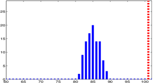
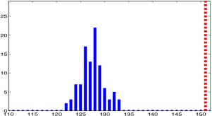
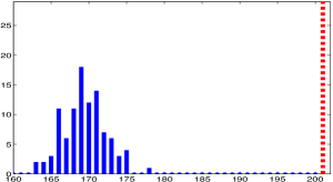
and we use interior point methods as in SDPT3 [38] to solve (4.3). (Our simulations use CVX which in turn calls SDPT3.) This phenomenon is explained below. At the moment, we would like to remark that Condition (4.5) is sufficient for the primal problem (1.4) to have a unique solution, and holds except in very special cases. To illustrate this, suppose $y$ is a random vector, not a measurement vector corresponding to a sparse signal. In this case, we typically observe dual solutions as shown in Figure 10 (non-vanishing polynomials with at most $n-1$ roots). To be sure, we have solved 400 instances of (4.3) with different values of $f_{c}$ and random data $y$. In every single case, condition (4.5) held so that we could construct a primal feasible solution $x$ with a duality gap below $10^{-8}$, see Figure 11. In all instances, the support of $x$ was constructed by determining roots of $p_{2n-2}(z)$ at a distance at most $10^{-4}$ from the unit circle.

Figure 11: Primal feasible points $x$ with a duality gap below $10^{-8}$ are constructed from random data $y$ sampled with i.i.d. complex Gaussian entries. A dual gap below $10^{-8}$ implies that $\|x\|_{\text{TV}}-\|\hat{x}\|_{\text{TV}}\leq 10^{-8}$, where $\hat{x}$ is any primal optimal solution. (For reference, the optimal value $\|\hat{x}\|_{\text{TV}}$ is on the order of 10 in all cases.) Each figure plots the frequency of occurrence of support cardinalities out of 100 realizations. For example, in (a) we obtained a support size equal to 44 in 25 instances out of 100. The value of $n$ is the same in each plot and is marked by a dashed red line; (a) $n=51$, (b) $n=101$, (c) $n=151$, (d) $n=201$.

Interior point methods approach solutions from the interior of the feasible set by solving a sequence of optimization problems in which an extra term, a scaled barrier function, is added to the cost function [4]. To be more precise, in our case (4.3) would become

$$\max_{c,Q}\;\operatorname{Re}\left[y^{\ast}c\right]+t\log\det\left(\begin{bmatrix}Q&c\\ c^{\ast}&1\end{bmatrix}\right)\quad\text{subject to}\quad\text{\eqref{eq:sdp-charact}},$$ (4.6)

where $t$ is a positive parameter that is gradually reduced towards zero in order to approach a solution to (4.3). Let $\lambda_{k}$, $1\leq k\leq n$, denote the eigenvalues of $Q-cc^{\ast}$. By Schur’s formula (Theorem 1.1 in [40]) we have

$$\log\det\left(\begin{bmatrix}Q&c\\ c^{\ast}&1\end{bmatrix}\right) =\log\det\left(Q-cc^{\ast}\right)=\sum_{k=1}^{n}\log\lambda_{k}.$$

Suppose condition (4.5) holds. Then Corollary 4.1 states that there exists $\tilde{c}$ with the property that at least one eigenvalue of $Q-\tilde{c}\tilde{c}^{\ast}$ is bounded away from zero. This is the reason why in the limit $t\rightarrow 0$, (4.6) will construct a non-vanishing polynomial $p_{2n-2}$ with at most $n-1$ roots on the unit circle rather than the trivial solution $p_{2n-2}=0$ since in the latter case, all the eigenvalues of $Q-{c}{c}^{\ast}$ vanish. Hence, an interior-point method can be said to solve the primal problem (1.4) provided (4.5) holds.

To conclude, we have merely presented an informal discussion of a semidefinite programming approach to the minimum-total variation problem (1.4). It is beyond the scope of this paper to rigorously justify this approach—for example, one would need to argue that the root finding procedure can be made stable, at least under the conditions of our main theorem—and we leave this to future work along with extensions to noisy data.

5 Numerical experiments

To evaluate the minimum distance needed to guarantee exact recovery by $\ell_{1}$ minimization of any signal in $\mathbb{C}^{N}$, for a fixed $N$, we propose the following heuristic scheme:

• For a super-resolution factor $\text{SRF}=N/n$, we work with a partial DFT matrix $F_{n}$ with frequencies up to $f_{c}=\lfloor n/2\rfloor$. Fix a candidate minimum distance $\Delta$.

• Using a greedy algorithm, construct an adversarial support with elements separated by at least $\Delta$ by sequentially adding elements to the support. Each new element is chosen to minimize the condition number formed by the columns corresponding to the selected elements.

• Take the signal $x$ to be the singular vector corresponding to the smallest singular value of $F_{n}$ restricted to $T$.

• Solve the $\ell_{1}$-minimization problem (1.11) and declare that exact recovery occurs if the normalized error is below a threshold (in our case $10^{-4}$).

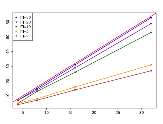
This construction of an adversarial signal was found to be better adapted to the structure of our measurement matrix than other methods proposed in the literature such as [14]. We used this scheme and a simple binary search to determine a lower bound for the minimum distance that guarantees exact recovery for $N=4096$, super-resolution factors of 8, 16, 32 and 64 and support sizes equal to 2, 5, 10, 20 and 50. The simulations were carried out in Matlab, using CVX [21] to solve the optimization problem. Figure 12 shows the results, which suggest that on the discrete grid we need at least a minimum distance equal to twice the super-resolution factor in order to guarantee reconstruction of the signal (red curve). Translated to the continuous setting, in which the signal would be supported on a grid with spacing $1/N$, this implies that $\Delta\gtrsim\lambda_{c}$ is a necessary condition for exact recovery.

Figure 12: Minimum distances (vertical axis) at which exact recovery by $\ell_{1}$ minimization occurs for the adversarial complex sign patterns against the corresponding super-resolution factors. At the red curve, the minimum distance would be exactly equal to twice the super-resolution factor. Signal length is $N=4096$.

6 Discussion

In this paper, we have developed the beginning of a mathematical theory of super-resolution. In particular, we have shown that we can super-resolve ‘events’ such as spikes, discontinuity points, and so on with infinite precision from just a few low-frequency samples by solving convenient convex programs. This holds in any dimension provided that the distance between events is proportional to $1/f_{c}=\lambda_{c}$, where $f_{c}$ is the highest observed frequency; for instance, in one dimension, a sufficient condition is that the distance between events is at least $2\lambda_{c}$. Furthermore, we have proved that when such condition holds, stable recovery is possible whereas super-resolution—by any method whatsoever—is in general completely hopeless whenever events are at a distance smaller than about $\lambda_{c}/2$.

6.1 Improvement

In one dimension, Theorem 1.2 shows that a sufficient condition for perfect super-resolution is $\Delta(T)\geq 2\,\lambda_{c}$. Furthermore, the authors of this paper have a proof showing that $\Delta(T)\geq 1.85\,\lambda_{c}$ is sufficient. This proof, however, is longer and more technical and, therefore, not presented here. In fact, we expect that arguments more sophisticated than those presented here would allow to lower this value even further. On the other hand, our numerical experiments show that we need at least $\Delta(T)\geq\lambda_{c}$ as one can otherwise find sparse signals which cannot be recovered by $\ell_{1}$ minimization. Hence, the minimum separation needed for success is somewhere between $\lambda_{c}$ and $1.85\,\lambda_{c}$. It would be interesting to know where this critical value might be.

6.2 Extensions

We have focused in this paper on the super-resolution of point sources, and by extension of discontinuity points in the function value, or in the derivative and so on. Clearly, there are many other models one could consider as well. For instance, we can imagine collecting low-frequency Fourier coefficients of a function

$$f(t)=\sum_{j}x_{j}\varphi_{j}(t),$$

where $\{\varphi_{j}(t)\}$ are basis functions. Again, $f$ may have lots of high-frequency content but we are only able to observe the low-end of the spectrum. An interesting research question is this: suppose the coefficient sequence $x$ is sparse, then under what conditions is it possible to super-resolve $f$ and extrapolate its spectrum accurately? In a different direction, it would be interesting to extend our stability results to other noise models and error metrics. We leave this to further research.

Acknowledgements

E. C. is partially supported by NSF via grant CCF-0963835 and the 2006 Waterman Award, by AFOSR under grant FA9550-09-1-0643 and by ONR under grant N00014-09-1-0258. C. F. is supported by a Caja Madrid Fellowship and was previously supported by a La Caixa Fellowship. E. C. would like to thank Mikhail Kolobov for fruitful discussions, and Mark Davenport, Thomas Strohmer and Vladislav Voroninski for useful comments about an early version of the paper. C. F. would like to thank Armin Eftekhari for a remark on Lemma 2.6.

Appendix A Background on the recovery of complex measures

With $\mathbb{T}=[0,1]$, the total variation of a complex measure $\nu$ on a set $B\in\mathcal{B}\left(\mathbb{T}\right)$ is defined by

$$\left|\nu\right|\left(B\right)=\sup\sum_{j=1}^{\infty}\left|\nu\left(B_{j}\right)\right|,$$

where the supremum is taken over all partitions of $B$ into a finite number of disjoint measurable subsets. The total variation $\left|\nu\right|$ is a positive measure on $\mathcal{B}\left(\mathbb{T}\right)$ and can be used to define the total-variation norm on the space of complex measures on $\mathcal{B}\left(\mathbb{T}\right)$,

$$\left|\left|\nu\right|\right|_{\text{TV}}=\left|\nu\right|\left(\mathbb{T}\right).$$

For further details, we refer the reader to [34].

Proposition A.1

Suppose that for any vector $v\in\mathbb{C}^{\left|T\right|}$ with unit-magnitude entries, there exists a low-frequency polynomial $q$ (2.1) obeying (2.2). Then $x$ is the unique solution to (1.4).

Proof The proof is a variation on the well-known argument for finite signals, and we note that a proof for continuous-time signals, similar to that below, can be found in [9]. Let $\hat{x}$ be a solution to (1.4) and set $\hat{x}=x+h$. Consider the Lebesgue decomposition of $h$ relative to $\left|x\right|$,

$$h=h_{T}+h_{T^{c}}\text{,}$$

where (1) $h_{T}$ and $h_{T^{c}}$ is a unique pair of complex measures on $\mathcal{B}\left(\mathbb{T}\right)$ such that $h_{T}$ is absolutely continuous with respect to $\left|x\right|$, and (2) $h_{T^{c}}$ and $\left|x\right|$ are mutually singular. It follows that $h_{T}$ is concentrated on $T$ while $h_{T^{c}}$ is concentrated on $T^{c}$. Invoking a corollary of the Radon-Nykodim Theorem (see Theorem 6.12 in [34]), it is possible to perform a polar decomposition of $h_{T}$:

$$h_{T}=e^{i2\pi\phi\left(t\right)}\left|h_{T}\right|\text{,}$$

such that $\phi\left(t\right)$ is a real function defined on $\mathbb{T}$. Assume that there exists $q(t)=\sum_{j=-f_{c}}^{f_{c}}a_{j}e^{-i2\pi jt}$ obeying

$$\begin{cases}q\left(t_{j}\right)=e^{-i2\pi\phi\left(t_{j}\right)},&\forall t_{j}\in T\\ \left|q\left(t\right)\right|<1,&\forall t\in[0,1]\setminus T.\end{cases}$$ (A.1)

The existence of $q$ suffices to establish a valuable inequality between the total-variation norms of $h_{T}$ and $h_{T^{c}}$. Begin with

$$0=\int_{\mathbb{T}}q(t)h(\text{d}t)=\int_{\mathbb{T}}q(t)h_{T}(\text{d}t)+\int_{\mathbb{T}}q(t)h_{T^{c}}(\text{d}t)=\left|\left|h_{T}\right|\right|_{\text{TV}}+\int_{\mathbb{T}}q(t)h_{T^{c}}(\text{d}t)$$

and observe that

$$\left|\int_{\mathbb{T}}q(t)h_{T^{c}}(\text{d}t)\right|<\left|\left|h_{T^{c}}\right|\right|_{\text{TV}}$$

provided $h_{T^{c}}\neq 0$. This gives

$$\left|\left|h_{T}\right|\right|_{\text{TV}}\leq\left|\left|h_{T^{c}}\right|\right|_{\text{TV}}$$

with a strict inequality if $h\neq 0$. Assuming $h\neq 0$, we have

$$\left|\left|x\right|\right|_{\text{TV}}\geq\left|\left|x+h\right|\right|_{\text{TV}}=\left|\left|x+h_{T}\right|\right|_{\text{TV}}+\left|\left|h_{T^{c}}\right|\right|_{\text{TV}}\geq\left|\left|x\right|\right|_{\text{TV}}-\left|\left|h_{T}\right|\right|_{\text{TV}}+\left|\left|h_{T^{c}}\right|\right|_{\text{TV}}>\left|\left|x\right|\right|_{\text{TV}}.$$

This is a contradiction and thus $h=0$. In other words, $x$ is the unique minimizer.  

Appendix B Proof of Lemma 2.6

The first inequality in the lemma holds due to two lower bounds on the sine function:

$$\left|\sin\left(\pi t\right)\right| \geq 2\left|t\right|,\text{ for all }t\in[-1/2,1/2]$$ (B.1)

$$\sin\left(\pi t\right) \geq\pi t-\frac{\pi^{3}t^{3}}{6}=\frac{2t}{a(t)},\text{ for all }t\geq 0.$$ (B.2)

The proof for these expressions, which we omit, is based on concavity of the sine function and on a Taylor expansion around the origin. Put $f=f_{c}/2+1$ for short. Some simple calculations give $K^{\prime}(0)=0$ and for $t\neq 0$,

$$K^{\prime}\left(t\right)=4\pi\left(\frac{\sin\left(f\pi t\right)}{f\sin\left(\pi t\right)}\right)^{3}\left(\frac{\cos\left(f\pi t\right)}{\sin\left(\pi t\right)}-\frac{\sin\left(f\pi t\right)\cos\left(\pi t\right)}{f\sin^{2}\left(\pi t\right)}\right).$$ (B.3)

Further calculations show that the value of the second derivative of $K$ at the origin is $-\pi^{2}f_{c}\left(f_{c}+4\right)/3$, and for $t\neq 0$,

$$K^{\prime\prime}\left(t\right)=\frac{4\pi^{2}\sin^{2}\left(f\pi t\right)}{f^{2}\sin^{4}\left(\pi t\right)}\left[3\left(\cos\left(f\pi t\right)-\frac{\sin\left(f\pi t\right)\cos\left(\pi t\right)}{f\sin\left(\pi t\right)}\right)^{2}\right.\\ \left.-\sin^{2}\left(f\pi t\right)-\frac{\sin\left(2f\pi t\right)}{f\tan\left(\pi t\right)}+\frac{\sin^{2}\left(f\pi t\right)}{f^{2}\tan^{2}\left(\pi t\right)}+\frac{\sin^{2}\left(f\pi t\right)}{f^{2}\sin^{2}\left(\pi t\right)}\right].$$ (B.4)

It is also possible to check that the third derivative of $K$ is zero at the origin, and for $t\neq 0$,

$$K^{\prime\prime\prime}\left(t\right)=\frac{4\pi^{3}\sin\left(f\pi t\right)}{f\sin^{4}\left(\pi t\right)}\,\left(6H_{1}(t)+9\sin\left(f\pi t\right)H_{2}(t)+\sin^{2}\left(f\pi t\right)H_{3}(t)\right)$$ (B.5)

with

$$H_{1}(t) =\left(\cos\left(f\pi t\right)-\frac{\sin\left(f\pi t\right)\cos\left(\pi t\right)}{f\sin\left(\pi t\right)}\right)^{3}$$

$$H_{2}(t) =\left(\cos\left(f\pi t\right)-\frac{\sin\left(f\pi t\right)\cos\left(\pi t\right)}{f\sin\left(\pi t\right)}\right)\left(-\sin\left(f\pi t\right)-\frac{2\cos\left(f\pi t\right)}{f\tan\left(\pi t\right)}+\frac{\sin\left(f\pi t\right)}{f^{2}\tan^{2}\left(\pi t\right)}+\frac{\sin\left(f\pi t\right)}{f^{2}\sin^{2}\left(\pi t\right)}\right)$$

$$H_{3}(t) =\left(\frac{3\cos\left(f\pi t\right)\left(1+\cos^{2}\left(\pi t\right)\right)}{f^{2}\sin^{2}\left(\pi t\right)}-\cos\left(f\pi t\right)+\frac{3\sin\left(f\pi t\right)}{f\tan\left(\pi t\right)}-\frac{\sin\left(f\pi t\right)\left(1+5\cos\left(\pi t\right)\right)}{f^{3}\sin^{3}\left(\pi t\right)}\right).$$

The remaining inequalities in the lemma are all almost direct consequences of plugging (B.1) and (B.2) into (B.3), (B.4) and (B). The bounds are nonincreasing in $t$ because the derivative of $b(t)$ is negative between zero and $\sqrt{2}/\pi$ and one can check that $H_{\ell}(\sqrt{2}/\pi)<H_{\ell}^{\infty}$ for $f_{c}\geq 128$. Additionally, $b^{k}(t)$ is strictly convex for positive $t$ and $k\in\left\{1,2,3\right\}$, so the derivative with respect to $\tau$ of $b^{k}(\Delta-\tau)+b^{k}(\Delta+\tau)$ is positive for $0\leq\tau<\Delta/2$, which implies that $\tilde{B}_{\ell}(\Delta-\tau)+\tilde{B}_{\ell}(\Delta+\tau)$ is increasing in $\tau$.

Appendix C Proof of Theorem 1.3

Theorem 1.3 follows from Proposition C.1 below, which guarantees the existence of a dual certificate. In this section, we write $\Delta=\Delta(T)\geq\Delta_{\text{min}}=2.38\,\lambda_{c}$. Unless specified otherwise, $|r-r^{\prime}|$ is the $\infty$ distance.

Proposition C.1

Let $T=\left\{r_{1},r_{2},\dots\right\}\subset\mathbb{T}^{2}$ be any family of points obeying the minimum distance condition

$$\left|r_{j}-r_{k}\right|\geq 2.38\,\lambda_{c},\quad r_{j}\neq r_{k}\in T.$$

Assume $f_{c}\geq 512$. Then for any vector $v\in\mathbb{R}^{\left|T\right|}$ with $\left|v_{j}\right|=1$, there exists a trigonometric polynomial $q$ with Fourier series coefficients supported on $\{-f_{c},-f_{c}+1,\ldots,f_{c}\}^{2}$ with the property

$$\begin{cases}q(r_{j})=v_{j},&t_{j}\in T,\\ |q(r)|<1,&t\in\mathbb{T}^{2}\setminus T.\end{cases}$$ (C.1)

The proof is similar to that of Proposition 2.1 in that we shall construct the dual polynomial $q$ by interpolation with a low-pass, yet rapidly decaying two-dimensional kernel. Here, we consider

$$K^{\text{2D}}\left(r\right)=K\left(x\right)K\left(y\right)\text{,}$$

obtained by tensorizing the square of the Fejer kernel (2.3). (For reference, if we had data in which $y(k)$ is observed if $\|k\|_{2}\leq f_{c}$, we would probably use a radial kernel.) Just as before, we have fixed $K$ somewhat arbitrarily, and it would probably be possible to optimize this choice to improve the constant factor in the expression for the minimum distance. We interpolate the sign pattern using $K^{\text{2D}}$ and its partial derivatives, denoted by $K^{\text{2D}}_{\left(1,0\right)}$ and $K^{\text{2D}}_{\left(0,1\right)}$ respectively, as follows:

$$q\left(r\right)=\sum_{r_{j}\in T}\bigl{[}\alpha_{j}K^{\text{2D}}\left(r-r_{j}\right)+\beta_{1j}K^{\text{2D}}_{\left(1,0\right)}\left(r-r_{j}\right)+\beta_{2j}K^{\text{2D}}_{\left(0,1\right)}\left(r-r_{j}\right)\bigr{]},$$

and we fit the coefficients so that for all $t_{j}\in T$,

$$q\left(t_{j}\right) =v_{j},$$ (C.2)

$$\nabla q\left(t_{j}\right) =0.$$

The first intermediate result shows that the dual polynomial is well defined, and also controls the magnitude of the interpolation coefficients.

Lemma C.2

Under the hypotheses of Proposition C.1, there are vectors $\alpha$, $\beta_{1}$ and $\beta_{2}$ obeying (C.2) and

$$\left|\left|\alpha\right|\right|_{\infty} \leq 1+5.577\;10^{-2},$$ (C.3)

$$\left|\left|\beta\right|\right|_{\infty} \leq 2.930\;10^{-2}\,\lambda_{c},$$

where $\beta=(\beta_{1},\beta_{2})$. Further, if $v_{1}=1$,

$$\alpha_{1} \geq 1-5.577\;10^{-2}\text{.}$$ (C.4)

Proposition C.1 is now a consequence of the two lemmas below which control the size of $q$ near a point $r_{0}\in T$. Without loss of generality, we can take $r_{0}=0$.

Lemma C.3

Assume $0\in T$. Then under the hypotheses of Proposition C.1, $\left|q\left(r\right)\right|<1$ for all $0<|r|\leq 0.2447\,\lambda_{c}$.

Lemma C.4

Assume $0\in T$. Then under the conditions of Proposition C.1, $\left|q\left(r\right)\right|<1$ for all $r$ obeying $0.2447\,\lambda_{c}\leq\left|r\right|\leq\Delta/2$. This also holds for all $r$ that are closer to $0\in T$ (in the $\infty$ distance) than to any other element in $T$.

C.1 Proof of Lemma C.2

To express the interpolation constraints in matrix form, define

$$\left(D_{0}\right)_{jk} =K^{\text{2D}}\left(r_{j}-r_{k}\right), \qquad\left(D_{\left(1,0\right)}\right)_{jk} =K^{\text{2D}}_{\left(1,0\right)}\left(r_{j}-r_{k}\right), \qquad\left(D_{\left(0,1\right)}\right)_{jk} =K^{\text{2D}}_{\left(0,1\right)}\left(r_{j}-r_{k}\right),$$

$$\left(D_{\left(1,1\right)}\right)_{jk} =K^{\text{2D}}_{\left(1,1\right)}\left(r_{j}-r_{k}\right), \qquad\left(D_{\left(2,0\right)}\right)_{jk} =K^{\text{2D}}_{\left(2,0\right)}\left(r_{j}-r_{k}\right), \qquad\left(D_{\left(0,2\right)}\right)_{jk} =K^{\text{2D}}_{\left(0,2\right)}\left(r_{j}-r_{k}\right)\text{.}$$

To be clear, $K^{\text{2D}}_{(\ell_{1},\ell_{2})}$ means that we are taking $\ell_{1}$ and $\ell_{2}$ derivatives with respect to the first and second variables. Note that $D_{0}$, $D_{\left(2,0\right)}$, $D_{\left(1,1\right)}$ and $D_{\left(0,2\right)}$ are symmetric, while $D_{\left(1,0\right)}$ and $D_{\left(0,1\right)}$ are antisymmetric, because $K$ and $K^{\prime\prime}$ are even while $K^{\prime}$ is odd. The interpolation coefficients are solutions to

$$\begin{bmatrix}D_{0}&D_{\left(1,0\right)}&D_{\left(0,1\right)}\\ D_{\left(1,0\right)}&D_{\left(2,0\right)}&D_{\left(1,1\right)}\\ D_{\left(0,1\right)}&D_{\left(1,1\right)}&D_{\left(0,2\right)}\end{bmatrix}\begin{bmatrix}\alpha\\ \beta_{1}\\ \beta_{2}\end{bmatrix} =\begin{bmatrix}v\\ 0\\ 0\end{bmatrix}\quad\Leftrightarrow\quad\begin{bmatrix}D_{0}&-\tilde{D}_{1}^{T}\\ \tilde{D}_{1}&\tilde{D}_{2}\end{bmatrix}\begin{bmatrix}\alpha\\ \beta\end{bmatrix}=\begin{bmatrix}v\\ 0\end{bmatrix}\text{,}$$ (C.5)

where we have defined two new matrices $\tilde{D}_{1}$ and $\tilde{D}_{2}$. The norm of these matrices can be bounded by leveraging 1D results. For instance, consider

$$\left|\left|\text{\em I}-D_{0}\right|\right|_{\infty}=\sum_{r_{j}\in T\setminus\{0\}}\left|K^{\text{2D}}\left(r_{j}\right)\right|.$$

We split this sum into different regions corresponding to whether $|x_{j}|$ or $|y_{j}|\leq\Delta/2$ and to $\min(|x_{j}|,|y_{j}|)\geq\Delta/2$. First,

$$\sum_{r_{j}\neq 0\,:\,|y_{j}|<\Delta/2}\left|K^{\text{2D}}\left(r_{j}\right)\right|\leq\sum_{r_{j}\neq 0\,:\,|y_{j}|<\Delta/2}B_{0}\left(x_{j}\right)\leq 2\sum_{j\geq 1}B_{0}(j\Delta).$$

This holds because the $x_{j}$’s must be at least $\Delta$ apart, $B_{0}$ is nonincreasing and the absolute value of $K^{\text{2D}}$ is bounded by one. The region $\{r_{j}\neq 0,\,|x_{j}|<\Delta/2\}$ yields the same bound. Now observe that Lemma C.5 below combined with Lemma 2.6 gives

$$\sum_{r_{j}\neq 0\,:\,\min(x_{j},y_{j})\geq\Delta/2}\left|K^{\text{2D}}\left(r_{j}\right)\right|\leq\sum_{r_{j}\neq 0\,:\,\min(x_{j},y_{j})\geq\Delta/2}B_{0}\left(x_{j}\right)B_{0}\left(y_{j}\right)\leq\Bigl{[}\sum_{j_{1}\geq 0}B_{0}(\Delta/2+j_{1}\Delta)\Bigr{]}^{2}.$$

To bound this expression, we apply the exact same technique as for (2.11) in Section 2.3, starting at $j=0$ and setting $j_{0}=20$. This gives

$$\left|\left|\text{\em I}-D_{0}\right|\right|_{\infty}\leq 4\sum_{j\geq 1}B_{0}(j\Delta)+4\Bigl{[}\sum_{j\geq 0}B_{0}(\Delta/2+j\Delta)\Bigr{]}^{2}\leq 4.854\;10^{-2}.$$ (C.6)

Lemma C.5

Suppose $x\in\mathbb{R}_{+}^{2}$ and $f(x)=f_{1}(x_{1})f_{2}(x_{2})$ where both $f_{1}$ and $f_{2}$ are nonincreasing. Consider any collection of points $\{x_{j}\}\subset\mathbb{R}^{2}_{+}$ for which $|x_{i}-x_{j}|\geq 1$. Then

$$\sum_{j}f(x_{j})\leq\sum_{j_{1}\geq 0}f_{1}(j_{1})\sum_{j_{2}\geq 0}f_{2}(j_{2}).$$

Proof Consider the mapping $x\in\mathbb{R}^{2}_{+}\mapsto(\lfloor x_{1}\rfloor,\lfloor x_{2}\rfloor)$. This mapping is injective over our family of points. (Indeed, two points cannot be mapped to the same pair of integers $(j_{1},j_{2})$ as it would otherwise imply that they are both inside the square $[j_{1}+1)\times[j_{2}+1)$, hence violating the separation condition.) Therefore, the monotonicity assumption gives

$$\sum_{j}f(x_{j})\leq\sum_{j}f_{1}(\lfloor x_{j,1}\rfloor)f_{2}(\lfloor x_{j,2}\rfloor)\leq\sum_{j_{1},j_{2}\geq 0}f_{1}(j_{1})f_{2}(j_{2}),$$

which proves the claim.  

Applying the same reasoning, we obtain

$$\left|\left|D_{\left(1,0\right)}\right|\right|_{\infty}\leq 2\sum_{j\geq 1}B_{1}(j\Delta)+2\|K^{\prime}\|_{\infty}\sum_{j\geq 1}B_{0}(j\Delta)+4\Bigl{[}\sum_{j\geq 0}B_{0}(\Delta/2+j\Delta)\Bigr{]}\Bigl{[}\sum_{j\geq 0}B_{1}(\Delta/2+j\Delta)\Bigr{]}.$$

In turn, the same upper-bounding technique yields

$$\left|\left|D_{\left(1,0\right)}\right|\right|_{\infty}\leq 7.723\;10^{-2}\,f_{c},$$ (C.7)

where we have used the fact that $\|K^{\prime}\|_{\infty}\leq 2.08\left(f_{c}+2\right)$, which follows from combining Lemma 2.6 with (2.21). Likewise,

$$\left|\left|D_{\left(1,1\right)}\right|\right|_{\infty}\leq 4\|K^{\prime}\|_{\infty}\sum_{j\geq 1}B_{1}(j\Delta)+4\Bigl{[}\sum_{j\geq 0}B_{1}(\Delta/2+j\Delta)\Bigr{]}^{2}\leq 0.1576\,f_{c}^{2},$$ (C.8)

and finally,

$$\left|\left|\left|K^{\text{2D}}_{\left(2,0\right)}\left(0\right)\right|\text{\em I}-D_{\left(2,0\right)}\right|\right|_{\infty}\leq 2\sum_{j\geq 1}B_{2}(j\Delta)+2\|K^{\prime\prime}\|_{\infty}\sum_{j\geq 1}B_{0}(j\Delta)\\ +4\Bigl{[}\sum_{j\geq 0}B_{0}(\Delta/2+j\Delta)\Bigr{]}\Bigl{[}\sum_{j\geq 0}B_{2}(\Delta/2+j\Delta)\Bigr{]}\leq 0.3539\,f_{c}^{2},$$ (C.9)

since $\|K^{\prime\prime}\|_{\infty}=\pi^{2}f_{c}\left(f_{c}+4\right)/3$, as $\left|K^{\prime\prime}\right|$ reaches its global maximum at the origin.

We use these estimates to show that the system (C.5) is invertible and to show that the coefficient sequences are bounded. To ease notation, set

$$S_{1} =D_{\left(2,0\right)}-D_{\left(1,1\right)}D_{\left(0,2\right)}^{-1}D_{\left(1,1\right)},$$

$$S_{2} =D_{\left(1,0\right)}-D_{\left(1,1\right)}D_{\left(0,2\right)}^{-1}D_{y},$$

$$S_{3} =D_{0}+S_{2}^{T}S_{1}^{-1}S_{2}-D_{\left(0,1\right)}D_{\left(0,2\right)}^{-1}D_{\left(0,1\right)}\text{.}$$

Note that $S_{1}$ is a Schur complement of $D_{\left(0,2\right)}$ and that a standard linear algebra identity gives

$$\tilde{D}_{2}^{-1} =\begin{bmatrix}S_{1}^{-1}&-S_{1}^{-1}D_{\left(1,1\right)}D_{\left(0,2\right)}^{-1}\\ -D_{\left(0,2\right)}^{-1}D_{\left(1,1\right)}S_{1}^{-1}&D_{\left(0,2\right)}^{-1}+D_{\left(0,2\right)}^{-1}D_{\left(1,1\right)}S_{1}^{-1}D_{\left(1,1\right)}D_{\left(0,2\right)}^{-1}\end{bmatrix}\text{.}$$

Using this and taking the Schur complement of $\tilde{D}_{2}$, which is equal to $S_{3}$, the solution to (C.5) can be written as

$$\begin{bmatrix}\alpha\\ \beta\end{bmatrix} =\begin{bmatrix}\text{\em I}\\ -\tilde{D}_{2}^{-1}\tilde{D}_{1}\end{bmatrix}\left(D_{0}+\tilde{D}_{1}^{T}\tilde{D}_{2}^{-1}\tilde{D}_{1}\right)^{-1}v\quad\Leftrightarrow\quad\begin{bmatrix}\alpha\\ \beta_{1}\\ \beta_{2}\end{bmatrix}=\begin{bmatrix}\text{\em I}\\ -S_{1}^{-1}S_{2}\\ D_{\left(0,2\right)}^{-1}\left(D_{\left(1,1\right)}S_{1}^{-1}S_{2}-D_{\left(0,1\right)}\right)\end{bmatrix}S_{3}^{-1}v\text{.}$$

Applying (2.13) from Section 2.3.1, we obtain

$$\left|\left|D_{\left(0,2\right)}^{-1}\right|\right|_{\infty} \leq\frac{1}{\left|K^{\text{2D}}_{\left(0,2\right)}\left(0\right)\right|-\left|\left|\left|K^{\text{2D}}_{\left(0,2\right)}\left(0\right)\right|\text{\em I}-D_{\left(0,2\right)}\right|\right|_{\infty}}\leq\frac{0.3399}{f_{c}^{2}}\text{,}$$ (C.10)

which together with $K^{\text{2D}}_{\left(2,0\right)}\left(0\right)=-\pi^{2}f_{c}\left(f_{c}+4\right)/3$ and (C.8) imply

$$\left|\left|\left|K^{\text{2D}}_{\left(2,0\right)}\left(0\right)\right|\text{\em I}-S_{1}\right|\right|_{\infty} \leq\left|\left|\left|K^{\text{2D}}_{\left(2,0\right)}\left(0\right)\right|\text{\em I}-D_{\left(2,0\right)}\right|\right|_{\infty}+\left|\left|D_{\left(1,1\right)}\right|\right|_{\infty}^{2}\left|\left|D_{\left(0,2\right)}^{-1}\right|\right|_{\infty}\leq 0.33624\,f_{c}^{2}\text{.}$$

Another application of (2.13) then yields

$$\left|\left|S_{1}^{-1}\right|\right|_{\infty} \leq\frac{1}{\left|K^{\text{2D}}_{\left(2,0\right)}\left(0\right)\right|-\left|\left|\left|K^{\text{2D}}_{\left(2,0\right)}\left(0\right)\right|\text{\em I}-S_{1}\right|\right|_{\infty}}\leq\frac{0.3408}{f_{c}^{2}}\text{.}$$ (C.11)

Next, (C.7), (C.8) and (C.10) allow to bound $S_{2}$,

$$\left|\left|S_{2}\right|\right|_{\infty} \leq\left|\left|D_{\left(1,0\right)}\right|\right|_{\infty}+\left|\left|D_{\left(1,1\right)}\right|\right|_{\infty}\left|\left|D_{\left(0,2\right)}^{-1}\right|\right|_{\infty}\left|\left|D_{\left(0,1\right)}\right|\right|_{\infty}\leq 8.142\;10^{-2}\,f_{c}\text{,}$$

which combined with (C.6), (C.7), (C.10) and (C.11) implies

$$\left|\left|\text{\em I}-S_{3}\right|\right|_{\infty} \leq\left|\left|\text{\em I}-D_{0}\right|\right|_{\infty}+\left|\left|S_{2}\right|\right|_{\infty}^{2}\left|\left|S_{1}^{-1}\right|\right|_{\infty}+\left|\left|D_{\left(0,1\right)}\right|\right|_{\infty}^{2}\left|\left|D_{\left(0,2\right)}^{-1}\right|\right|_{\infty}\leq 5.283\;10^{-2}\text{.}$$

The results above allow us to derive bounds on the coefficient vectors by applying (2.13) one last time, establishing

$$\left|\left|\alpha\right|\right|_{\infty} \leq\left|\left|S_{3}^{-1}\right|\right|_{\infty}\leq 1+5.577\;10^{-2},$$

$$\left|\left|\beta_{1}\right|\right|_{\infty} \leq\left|\left|S_{1}^{-1}S_{2}S_{3}^{-1}\right|\right|_{\infty}\leq\left|\left|S_{1}^{-1}\right|\right|_{\infty}\left|\left|S_{2}\right|\right|_{\infty}\left|\left|S_{3}^{-1}\right|\right|_{\infty}\leq 2.930\;10^{-2}\,\lambda_{c},$$

$$\alpha_{1} =v_{1}-\left(\left(\text{\em I}-S_{3}^{-1}\right)v\right)_{1}\geq 1-\left|\left|S_{3}^{-1}\right|\right|_{\infty}\left|\left|\text{\em I}-S_{3}\right|\right|_{\infty}\geq 1-5.577\;10^{-2}\text{,}$$

where the last lower bound holds if $v_{1}=1$. The derivation for $\left|\left|\beta_{2}\right|\right|_{\infty}$ is identical and we omit it.

C.2 Proof of Lemma C.3

Since $v$ is real valued, $\alpha$, $\beta$ and $q$ are all real valued. For $|r|\leq 0.2447\,\lambda_{c}$, we show that the Hessian matrix of $q$,

$$H=\begin{bmatrix}q_{\left(2,0\right)}\left(r\right)&q_{\left(1,1\right)}\left(r\right)\\ q_{\left(1,1\right)}\left(r\right)&q_{\left(0,2\right)}\left(r\right)\end{bmatrix}$$

is negative definite. In what follows, it will also be useful to establish bounds on the kernel and its derivatives near the origin. Using (2.20)–(2.24), we obtain

$$K^{\text{2D}}\left(x,y\right) \geq\left(1-\frac{\pi^{2}f_{c}\left(f_{c}+4\right)x^{2}}{6}\right)\left(1-\frac{\pi^{2}f_{c}\left(f_{c}+4\right)y^{2}}{6}\right)$$

$$K^{\text{2D}}_{\left(2,0\right)}\left(x,y\right) \leq\left(-\frac{\pi^{2}f_{c}\left(f_{c}+4\right)}{3}+\frac{\left(f_{c}+2\right)^{4}\pi^{4}x^{2}}{6}\right)\left(1-\frac{\pi^{2}f_{c}\left(f_{c}+4\right)y^{2}}{6}\right)$$

and

$$\left|K^{\text{2D}}_{\left(1,0\right)}\left(x,y\right)\right| \leq\frac{\pi^{2}f_{c}\left(f_{c}+4\right)x}{3}, \qquad\left|K^{\text{2D}}_{\left(1,1\right)}\left(x,y\right)\right| \leq\frac{\pi^{4}f_{c}^{2}\left(f_{c}+4\right)^{2}xy}{9},$$

$$\left|K^{\text{2D}}_{\left(2,1\right)}\left(x,y\right)\right| \leq\frac{\pi^{4}f_{c}^{2}\left(f_{c}+4\right)^{2}y}{9}, \qquad\left|K^{\text{2D}}_{\left(3,0\right)}\left(x,y\right)\right| \leq\frac{\pi^{4}\left(f_{c}+2\right)^{4}x}{3}.$$

These bounds are all monotone in $x$ and $y$ so we can evaluate them at $x=0.2447\,\lambda_{c}$ and $y=0.2447\,\lambda_{c}$ to show that for any $|r|\leq 0.2447\,\lambda_{c}$,

$$K^{\text{2D}}\left(r\right) \geq 0.8113 \qquad\left|K^{\text{2D}}_{\left(1,0\right)}\left(r\right)\right| \leq 0.8113 \qquad K^{\text{2D}}_{\left(2,0\right)}\left(r\right) \leq-2.097\,f_{c}^{2},$$

$$\left|K^{\text{2D}}_{\left(1,1\right)}\left(r\right)\right| \leq 0.6531\,f_{c}, \qquad\left|K^{\text{2D}}_{\left(2,1\right)}\left(r\right)\right| \leq 2.669\,f_{c}^{2}, \qquad\left|K^{\text{2D}}_{\left(3,0\right)}\left(r\right)\right| \leq 8.070\,f_{c}^{3}.$$ (C.12)

The bounds for $K^{\text{2D}}_{\left(1,0\right)}$, $K^{\text{2D}}_{\left(2,0\right)}$, $K^{\text{2D}}_{\left(2,1\right)}$ and $K^{\text{2D}}_{\left(3,0\right)}$ of course also hold for $K^{\text{2D}}_{\left(0,1\right)}$, $K^{\text{2D}}_{\left(0,2\right)}$, $K^{\text{2D}}_{\left(1,2\right)}$ and $K^{\text{2D}}_{\left(0,3\right)}$. Additionally, it will be necessary to bound sums of the form $\sum_{r_{j}\in T/\left\{0\right\}}\left|K^{\text{2D}}_{\left(\ell_{1},\ell_{2}\right)}\left(r-r_{j}\right)\right|$ for $r$ such that $\left|r\right|\leq\Delta/2$ and $\ell_{1},\ell_{2}=0,1,2,3$. Consider the case $\left(\ell_{1},\ell_{2}\right)=\left(0,0\right)$. Without loss of generality, let $r=\left(x,y\right)\in\mathbb{R}_{+}^{2}$. By Lemma C.5, the contribution of those ${r_{j}}$’s belonging to the three quadrants $\{|r|>\Delta/2\}\setminus\mathbb{R}^{2}_{+}$ obeys

$$\sum_{|r_{j}|>\Delta/2,r_{j}\notin\mathbb{R}_{+}^{2}}\left|K^{\text{2D}}\left(r-r_{j}\right)\right|\leq 3\Bigl{[}\sum_{j\geq 0}B_{0}(\Delta/2+j\Delta)\Bigr{]}^{2}.$$

Similarly, the contribution from the bands where either $|r_{j,1}|$ or $|r_{j,2}|\leq\Delta/2$ obeys

$$\sum_{|r_{j,1}|\leq\Delta/2\text{ or }|r_{j,2}|\leq\Delta/2}\left|K^{\text{2D}}\left(r-r_{j}\right)\right|\leq 2\sum_{j\geq 1}B_{0}(j\Delta-\left|r\right|).$$

It remains to bound the sum over $r_{j}$’s lying in the positive quadrant $\{|r|>\Delta/2\}\cap\mathbb{R}^{2}_{+}$. To do this, let $f_{1}\left(t\right)$ be equal to one if $\left|t\right|\leq\Delta$ and to $B_{0}(\Delta t-\left|r\right|)$ otherwise. Taking $f_{2}=f_{1}$, Lemma C.5 gives

$$\sum_{|r_{j}|>\Delta/2,r_{j}\in\mathbb{R}_{+}^{2}}\left|K^{\text{2D}}\left(r-r_{j}\right)\right|\leq\sum_{j\geq 1}B_{0}(j\Delta-\left|r\right|)+\Bigl{[}\sum_{j\geq 1}B_{0}(j\Delta-\left|r\right|)\Bigr{]}^{2}.$$

We can apply exactly the same reasoning to the summation of $K^{\text{2D}}_{\left(\ell_{1},\ell_{2}\right)}$ for other values of $\ell_{1}$ and $\ell_{2}$, and obtain that for any $r$ such that $\left|r\right|\leq\Delta/2$,

$$\sum_{r_{j}\in T\setminus\left\{0\right\}}\left|K^{\text{2D}}_{\left(\ell_{1},\ell_{2}\right)}\left(r-r_{j}\right)\right|\leq Z_{\left(\ell_{1},\ell_{2}\right)}\left(\left|r\right|\right);$$ (C.13)

here, for $u\geq 0$,

$$Z_{\left(\ell_{1},\ell_{2}\right)}\left(u\right) =2\sum_{j\geq 1}K^{\left(\ell_{1}\right)}_{\infty}B_{\ell_{2}}(j\Delta-u)+2K^{\left(\ell_{2}\right)}_{\infty}B_{\ell_{1}}(j\Delta-u)+K^{\left(\ell_{1}\right)}_{\infty}\sum_{j\geq 1}B_{\ell_{2}}(j\Delta)$$

$$\qquad+K^{\left(\ell_{2}\right)}_{\infty}\sum_{j\geq 1}B_{\ell_{1}}(j\Delta)+3\Bigl{[}\sum_{j\geq 0}B_{\ell_{1}}(\Delta/2+j\Delta)\Bigr{]}\Bigl{[}\sum_{j\geq 0}B_{\ell_{2}}(\Delta/2+j\Delta-u)\Bigr{]}$$

$$\qquad\qquad+\Bigl{[}\sum_{j\geq 1}B_{\ell_{1}}(j\Delta-u)\Bigr{]}\Bigl{[}\sum_{j\geq 1}B_{\ell_{2}}(j\Delta)\Bigr{]}$$

in which $K^{\left(\ell_{1}\right)}_{\infty}$ is a bound on the global maximum of $K^{\left(\ell_{1}\right)}$. The absolute value of the kernel $K$ and its second derivative reach their global maxima at the origin, so $K^{\left(0\right)}_{\infty}=1$ and $K^{\left(2\right)}_{\infty}=\pi^{2}f_{c}\left(f_{c}+4\right)/3$. Combining the bounds on $\left|K^{\prime}\right|$ and $\left|K^{\prime\prime\prime}\right|$ in Lemma 2.6 with (2.21) and (2.24), we can show that $K^{\left(1\right)}_{\infty}=2.08\left(f_{c}+2\right)$ and $K^{\left(3\right)}_{\infty}=25.3\left(f_{c}+2\right)^{3}$ if $f_{c}\geq 512$. Since $Z_{\left(\ell_{1},\ell_{2}\right)}=Z_{\left(\ell_{2},\ell_{1}\right)}$, we shall replace $Z_{\left(\ell_{1},\ell_{2}\right)}$ for which $\ell_{1}>\ell_{2}$ by $Z_{\left(\ell_{2},\ell_{1}\right)}$.

Since

$$q_{\left(2,0\right)}\left(r\right)=\sum_{r_{j}\in T}\alpha_{j}K^{\text{2D}}_{\left(2,0\right)}\left(r-r_{j}\right)+\beta_{1j}K^{\text{2D}}_{\left(3,0\right)}\left(r-r_{j}\right)+\beta_{2j}K^{\text{2D}}_{\left(2,1\right)}\left(r-r_{j}\right)$$

it follows from (C.12) and (C.13) that

$$q_{\left(2,0\right)}\left(r\right) \leq\alpha_{1}K^{\text{2D}}_{\left(2,0\right)}\left(r\right)+\left|\left|\alpha\right|\right|_{\infty}\sum_{r_{j}\in T\setminus\left\{0\right\}}\left|K^{\text{2D}}_{\left(2,0\right)}\left(r-r_{j}\right)\right|$$

$$\qquad+\left|\left|\beta\right|\right|_{\infty}\Bigl{[}\left|K^{\text{2D}}_{\left(3,0\right)}\left(r\right)\right|+\sum_{r_{j}\in T\setminus\left\{0\right\}}\left|K^{\text{2D}}_{\left(3,0\right)}\left(r-r_{j}\right)\right|+\left|K^{\text{2D}}_{\left(2,1\right)}\left(r\right)\right|+\sum_{r_{j}\in T\setminus\left\{0\right\}}\left|K^{\text{2D}}_{\left(2,1\right)}\left(r-r_{j}\right)\right|\Bigr{]}$$

$$\leq\alpha_{1}K^{\text{2D}}_{\left(2,0\right)}\left(r\right)+\left|\left|\alpha\right|\right|_{\infty}Z_{\left(0,2\right)}(|r|)+\left|\left|\beta\right|\right|_{\infty}\left(\left|K^{\text{2D}}_{\left(3,0\right)}\left(r\right)\right|+Z_{\left(0,3\right)}(|r|)+\left|K^{\text{2D}}_{\left(2,1\right)}\left(r\right)\right|+Z_{\left(1,2\right)}(|r|)\right)$$

$$\leq-1.175\,f_{c}^{2}.$$

The last inequality uses values of $Z_{\left(\ell_{1},\ell_{2}\right)}\left(u\right)$ at $u=0.2447\,\lambda_{c}$ reported in Table 6. By symmetry, the same bound holds for $q_{\left(0,2\right)}$. Finally, similar computations yield

$$\left|q_{\left(1,1\right)}(r)\right| =\sum_{r_{j}\in T}\alpha_{j}K^{\text{2D}}_{\left(1,1\right)}\left(r-r_{j}\right)+\beta_{1j}K^{\text{2D}}_{\left(2,1\right)}\left(r-r_{j}\right)+\beta_{2j}K^{\text{2D}}_{(1,2)}\left(r-r_{j}\right)$$

$$\leq\left|\left|\alpha\right|\right|_{\infty}\Bigl{[}\left|K^{\text{2D}}_{\left(1,1\right)}\left(r\right)\right|+Z_{(1,1)}(|r|)\Bigr{]}+\left|\left|\beta\right|\right|_{\infty}\Bigl{[}\left|K^{\text{2D}}_{\left(2,1\right)}\left(r\right)\right|+\left|K^{\text{2D}}_{\left(1,2\right)}\left(r\right)\right|+2Z_{(1,2)}(|r|)\Bigr{]}$$

$$\leq 1.059\,f_{c}^{2}.$$

Since $\operatorname{Tr}(H)=q_{\left(2,0\right)}+q_{\left(0,2\right)}<0$ and $\det(H)=|q_{\left(2,0\right)}||q_{\left(0,2\right)}|-|q_{\left(1,1\right)}|^{2}>0$, both eigenvalues of $H$ are strictly negative.

$Z_{\left(0,0\right)}(u)$	$Z_{\left(0,1\right)}(u)$	$Z_{\left(1,1\right)}(u)$	$Z_{\left(0,2\right)}(u)$	$Z_{\left(1,2\right)}(u)$	$Z_{\left(0,3\right)}(u)$
$6.405\;10^{-2}$	$0.1047\,f_{c}$	$0.1642\,f_{c}^{2}$	$0.4019\,f_{c}$	$0.6751\,f_{c}^{3}$	$1.574f_{c}^{3}$

Table 6: Upper bounds on $Z_{\left(\ell_{1},\ell_{2}\right)}(u)$ at $0.2447\,\lambda_{c}$.

We have shown that $q$ decreases along any segment originating at $0$. To complete the proof, we must establish that $q>-1$ in the square. Similar computations show

$$q\left(r\right) =\sum_{r_{j}\in T}\alpha_{j}K^{\text{2D}}\left(r-r_{j}\right)+\beta_{1j}K^{\text{2D}}_{\left(1,0\right)}\left(r-r_{j}\right)+\beta_{2j}K^{\text{2D}}_{\left(0,1\right)}\left(r-r_{j}\right)$$

$$\geq\alpha_{1}K^{\text{2D}}\left(r\right)-\left|\left|\alpha\right|\right|_{\infty}Z_{\left(0,0\right)}(|r|)-\left|\left|\beta\right|\right|_{\infty}\left(\left|K^{\text{2D}}_{\left(0,1\right)}\left(r\right)\right|+\left|K^{\text{2D}}_{\left(1,0\right)}\left(r\right)\right|+2Z_{\left(0,1\right)}(|r|)\right)$$

$$\geq 0.6447.$$

C.3 Proof of Lemma C.4

For $0.2447\,\lambda_{c}\leq\left|r\right|\leq\Delta/2$,

$$\left|q\right| \leq\Bigl{|}\sum_{r_{j}\in T}\alpha_{j}K^{\text{2D}}\left(r-r_{j}\right)+\beta_{1j}K^{\text{2D}}_{\left(1,0\right)}\left(r-r_{j}\right)+\beta_{2j}K^{\text{2D}}_{\left(0,1\right)}\left(r-r_{j}\right)\Bigr{|}$$

$$\leq\left|\left|\alpha\right|\right|_{\infty}\Bigl{[}\left|K^{\text{2D}}\left(r\right)\right|+Z_{(0,0)}(|r|)\Bigr{]}+\left|\left|\beta\right|\right|_{\infty}\Bigl{[}\left|K^{\text{2D}}_{\left(1,0\right)}\left(r\right)\right|+\left|K^{\text{2D}}_{\left(0,1\right)}\left(r\right)\right|+2Z_{(0,1)}(|r|)\Bigr{]}.$$

Using the series expansion around the origin of $K$ and $K^{\prime}$ (2.29), we obtain that for $t_{1}\leq|r|\leq t_{2}$,

$$\left|K^{\text{2D}}\left(r\right)\right| \leq\left(1-\frac{\pi^{2}f_{c}\left(f_{c}+4\right)x^{2}}{6}+\frac{\pi^{4}\left(f_{c}+2\right)^{4}x^{4}}{72}\right)\left(1-\frac{\pi^{2}f_{c}\left(f_{c}+4\right)y^{2}}{6}+\frac{\pi^{4}\left(f_{c}+2\right)^{4}y^{4}}{72}\right)$$

$$\leq\left(1-\frac{\pi^{2}\left(1+\frac{2}{f_{c}}\right)^{2}t_{1}^{2}}{6}\left(1-\frac{\pi^{2}\left(1+\frac{2}{f_{c}}\right)^{2}t_{2}^{2}}{12}\right)\right)^{2},$$

$$\left|K^{\text{2D}}_{\left(1,0\right)}\left(r\right)\right| \leq\left(\frac{\pi^{2}f_{c}\left(f_{c}+4\right)t_{2}}{3}\right)^{2}\text{.}$$

The same bound holds for $K^{\text{2D}}_{\left(0,1\right)}$. Now set

$$W\left(r\right)=\alpha^{\infty}\left|K^{\text{2D}}\left(r\right)\right|+2\beta^{\infty}\left|K^{\text{2D}}_{\left(1,0\right)}\left(r\right)\right|$$

where $\alpha^{\infty}$ and $\beta^{\infty}$ are the upper bounds from Lemma C.2. The quantities reported in Table 7 imply that setting $\left\{t_{1},t_{2}\right\}$ to $\left\{0.1649\,\lambda_{c},0.27\,\lambda_{c}\right\}$, $\left\{0.27\,\lambda_{c},0.36\,\lambda_{c}\right\}$, $\left\{0.36\,\lambda_{c},0.56\,\lambda_{c}\right\}$ and $\left\{0.56\,\lambda_{c},0.84\,\lambda_{c}\right\}$ yields $\left|q\right|<0.9958$, $\left|q\right|<0.9929$, $\left|q\right|<0.9617$ and $\left|q\right|<0.9841$ respectively in the corresponding intervals. Finally, for $\left|r\right|$ between $0.84\,\lambda_{c}$ and $\Delta/2$, applying Lemma (2.6) yields $W\left(r\right)\leq 0.5619$, $Z_{\left(0,0\right)}\left(0.84\,\lambda_{c}\right)\leq 0.3646$ and $Z_{\left(0,1\right)}\left(0.84\,\lambda_{c}\right)\leq 0.6502\,f_{c}$ , so that $\left|q\right|\leq 0.9850$. These last bounds also apply to any location beyond $\Delta/2$ closer to $0$ than to any other element of $T$ because of the monotonicity of $B_{0}$ and $B_{1}$. This concludes the proof.

$t_{1}/\lambda_{c}$	$t_{2}/\lambda_{c}$	Upper bound on $W\left(r\right)$	$Z_{\left(0,0\right)}\left(t_{2}\right)$	$Z_{\left(0,1\right)}\left(t_{2}\right)$
$0.2447$	$0.27$	$0.9203$	$6.561\,10^{-2}$	$0.1074$
$0.27$	$0.36$	$0.9099$	$7.196\,10^{-2}$	$0.1184$
$0.36$	$0.56$	$0.8551$	$9.239\,10^{-2}$	$0.1540$
$0.56$	$0.84$	$0.8118$	$0.1490$	$0.2547$

Table 7: Numerical quantities used to bound $\left|q\right|$ between $0.2447$ and $0.84$.

References

- [1] N. S. Banerjee and J. F. Geer. Exponentially accurate approximations to periodic Lipschitz functions based on Fourier series partial sums. J. Sci. Comput., 13:419–460, 1998.
- [2] D. Batenkov and Y. Yomdin. Algebraic Fourier reconstruction of piecewise smooth functions. Math. Comput., 81(277), 2012.
- [3] B. N. Bhaskar, G. Tang, and B. Recht. Atomic norm denoising with applications to line spectral estimation. Preprint.
- [4] S. Boyd and L. Vandenberghe. Convex Optimization. Cambridge University Press, 2004.
- [5] K. Bredies and H. K. Pikkarainen. Inverse problems in spaces of measures. ESAIM: Control, Optimisation and Calculus of Variations, 2012.
- [6] E. J. Candès, J. K. Romberg, and T. Tao. Robust uncertainty principles: exact signal reconstruction from highly incomplete frequency information. IEEE Transactions on Information Theory, 52(2):489–509, 2006.
- [7] E. J. Candès and T. Tao. Decoding by linear programming. IEEE Transactions on Information Theory, 51(12):4203–4215, 2005.
- [8] J. F. Claerbout and F. Muir. Robust modeling with erratic data. Geophysics, 38(5):826–844, 1973.
- [9] Y. de Castro and F. Gamboa. Exact reconstruction using Beurling minimal extrapolation. Preprint.
- [10] D. L. Donoho. Superresolution via sparsity constraints. SIAM J. Math. Anal., 23(5):1309–1331, 1992.
- [11] D. L. Donoho and P. B. Stark. Uncertainty principles and signal recovery. SIAM J. Appl. Math., 49:906–931, 1989.
- [12] D. L. Donoho and J. Tanner. Sparse nonnegative solutions of underdetermined linear equations by linear programming. In Proceedings of the National Academy of Sciences, pages 9446–9451, 2005.
- [13] C. Dossal. Estimation de fonctions gé˝́omé˝́triques et dé˝́convolution. PhD thesis, École Polytechnique, 2005.
- [14] C. Dossal, G. Peyré, and J. Fadili. A numerical exploration of compressed sampling recovery. In Proc. of SPARS’09, 2009.
- [15] P. Dragotti, M. Vetterli, and T. Blu. Sampling moments and reconstructing signals of finite rate of innovation: Shannon meets Strang-Fix. IEEE Transactions on Signal Processing, 55(5):1741–1757, 2007.
- [16] M. F. Duarte and R. G. Baraniuk. Spectral compressive sensing. Preprint.
- [17] B. Dumitrescu. Positive Trigonometric Polynomials and Signal Processing Applications. Springer, 2007.
- [18] K. S. Eckhoff. Accurate reconstructions of functions of finite regularity from truncated Fourier series expansions. Math. Comput., 64:671–690, 1995.
- [19] A. Fannjiang and W. Liao. Coherence-pattern guided compressive sensing with unresolved grids. SIAM J. Imaging Sci., 5:179, 2012.
- [20] J. J. Fuchs. Sparsity and uniqueness for some specific underdetermined linear systems. In Proc. of IEEE ICASSP 05, pages 729–732, 2005.
- [21] M. Grant and S. Boyd. CVX: Matlab software for disciplined convex programming, version 1.21. http://cvxr.com/cvx, 2011.
- [22] H. Greenspan. Super-resolution in medical imaging. Comput. J., 52:43–63, 2009.
- [23] T. D. Harris, R. D. Grober, J. K. Trautman, and E. Betzig. Super-resolution imaging spectroscopy. Appl. Spectrosc., 48(1):14A–21A, Jan 1994.
- [24] J. P. Kahane. Analyse et synthèse harmoniques. Preprint.
- [25] J. Kennedy, O. Israel, A. Frenkel, R. Bar-Shalom, and H. Azhari. Super-resolution in PET imaging. Medical Imaging, IEEE Transactions on, 25(2):137 –147, 2006.
- [26] V. Khaidukov, E. Landa, and T. J. Moser. Diffraction imaging by focusing-defocusing: An outlook on seismic superresolution. Geophysics, 69(6):1478–1490, 2004.
- [27] S. Levy and P. K. Fullagar. Reconstruction of a sparse spike train from a portion of its spectrum and application to high-resolution deconvolution. Geophysics, 46(9):1235–1243, 1981.
- [28] C. W. McCutchen. Superresolution in microscopy and the Abbe resolution limit. J. Opt. Soc. Am., 57(10):1190–1190, 1967.
- [29] J. Odendaal, E. Barnard, and C. Pistorius. Two-dimensional superresolution radar imaging using the MUSIC algorithm. Antennas and Propagation, IEEE Transactions on, 42(10):1386 –1391, 1994.
- [30] S. C. Park, M. K. Park, and M. G. Kang. Super-resolution image reconstruction: a technical overview. Signal Processing Magazine, IEEE, 20(3):21 – 36, 2003.
- [31] W. H. Press, S. A. Teukolsky, W. T. Vetterling, and B. P. Flannery. Numerical recipes in C (2nd ed.): the art of scientific computing. 1992.
- [32] K. G. Puschmann and F. Kneer. On super-resolution in astronomical imaging. Astronomy and Astrophysics, 436:373–378, 2005.
- [33] R. Rockafellar. Conjugate Duality and Optimization. Regional conference series in applied mathematics. Society for Industrial and Applied Mathematics, 1974.
- [34] W. Rudin. Real and complex analysis. McGraw-Hill Book Co., New York, 3rd edition, 1987.
- [35] F. Santosa and W. W. Symes. Linear inversion of band-limited reflection seismograms. SIAM Journal on Scientific and Statistical Computing, 7(4):1307–1330, 1986.
- [36] D. Slepian. Prolate spheroidal wave functions, Fourier analysis, and uncertainty. V - The discrete case. Bell System Technical Journal, 57:1371–1430, 1978.
- [37] V. Y. F. Tan and V. K. Goyal. Estimating signals with finite rate of innovation from noisy samples: A stochastic algorithm. Signal Processing, IEEE Transactions on, 56(10):5135–5146, 2008.
- [38] K. C. Toh, M. J. Todd, and R. H. Tütüncü. SDPT3 - a Matlab software package for semidefinite programming, Version 1.3. Optimization Methods and Software, 11(1):545–581, 1999.
- [39] J. A. Tropp. Just relax: convex programming methods for identifying sparse signals in noise. IEEE Transactions on Information Theory, 52(3):1030 –1051, 2006.
- [40] F. Zhang. The Schur Complement and Its Applications. Springer Science, 2005.