CHAOTICITY AND SHELL EFFECTS IN THE
NEAREST-NEIGHBOR DISTRIBUTIONS

Abstract

Statistics of the single-particle levels in a deformed Woods-Saxon potential is analyzed in terms of the Poisson and Wigner nearest-neighbor distributions for several deformations and multipolarities of its surface distortions. We found the significant differences of all the distributions with a fixed value of the angular momentum projection of the particle, more closely to the Wigner distribution, in contrast to the full spectra with Poisson-like behavior. Important shell effects are observed in the nearest neighbor spacing distributions, the larger the smaller deformations of the surface multipolarities.

PACS: 21.60. Sc, 21.10. -k, 21.10.Pc, 02.50. -r

I INTRODUCTION

The microscopic many-body interaction of particles of the Fermi systems such as heavy nuclei is rather complicated. Therefore, several theoretical approaches to the description of the Hamiltonian which are based on the statistical properties of its discrete levels are applied for solutions of the realistic problems. For a quantitative measure of the degree of chaoticity of the many-body forces, the statistical distributions of the spacing between the nearest neighboring levels were introduced, first of all in relation to the so called Random Matrix Theory porter ; wigner ; brody ; mehta ; aberg . Integrability (order) of the system was associated usually to the Poisson-like exponentially decreasing dependence on the spacing variable with a maximum at zero while chaoticity was connected more to the Wigner-like behavior with the zero spacing probability at zero but with a maximum at some finite value of this variable.

On the other hand, many dynamical problems, in particular, in nuclear physics can be reduced to the collective motion of independent particles in a mean field with a relatively sharp time-dependent edge called usually as the effective surface within the microscopic-macroscopic approximation myersswiat ; strut . We may begin with the basic ideas of Swiatecki and his collaborators myersswiat ; wall ; blsksw1 ; blshsw ; blsksw2 ; jasw ; maskbl . In recent years it became apparent that the collective nuclear dynamics is very much related to the nature of the nucleonic motion. This behavior of the nucleonic dynamics is important in physical processes like fission or heavy ion collisions where a great amount of the collective energy is dissipated into a chaotic nucleonic motion. We have to mention here also very intensive studies of the one-body dissipative phenomena described largely through the macroscopic wall formula (w.f.) for the excitation energy wall ; blsksw1 ; blsksw2 ; blshsw ; jasw ; maskbl and also quantum results blsksw1 ; blsksw2 ; maskbl ; kiev2010 . The analytical w.f. was suggested originally in Ref. wall on the basis of the Thomas-Fermi approach. It was re-derived in many works based on semiclassical and quantum arguments, see Refs koonrand ; maggzhfed ; gmf for instance. However, some problems in the analytical study of a multipolarity dependence of the smooth one-body friction and its oscillating corrections as functions of the particle number should be still clarified. In particular, we would like to emphasize the importance of the transparent classical picture through the Poincare sections and Lyapunov exponents showing the order-chaos transitions arvieu ; blshsw ; heiss ; heiss2 and also quantum results for the excitation energy blsksw2 ; maskbl ; kiev2010 . Then, the peculiarities of the excitation energies for many periods of the oscillations of the classical dynamics were discussed for several Legendre polynomials, see Ref. kiev2010 . as the classical measures of chaoticity. The shell correction method strut ; FH was successfully used to describe the shell effects in the nuclear deformation energies as functions of the particle numbers. This is important also for understanding analytically the origin of the isomers in fission within the periodic orbit theory (POT) myab . We should expect also that the deviations of the level density near the Fermi surface, like shell effects, from an averaged constant should influence essentially the nearest neighbor spacing distribution (NNSD). For a further study of the order-chaos properties of the Fermi systems, it might be worth to apply the statistical methods of the description of the single-particle (s.p.) levels of a mean-field Hamiltonian within microscopic-macroscopic approaches (see for instance Refs heiss1 ; heiss3 ; nazm1 ; nazm2 ).

The statistics of the spacing between the neighboring levels and their relation to the shell effects depending on the specific properties of the s.p. spectra, as well as the multipolarity and deformation of the shape surfaces should be expected. The quantitative measure of the order (or symmetry) can be the number of the single-valued integrals of motion, except for the energy (degree of the degeneracy of the system, see also Refs strutmag ; smod ; myab ; brbhad ). If the energy is the only one single-valued integral of motion one has the completely chaotic system gutz . For the case of any such additional integral of motion, say the angular momentum projection for the azimuthal symmetry, one finds the symmetry enhancement that is important for calculations of the level density as the basic s.p. characteristics.

Our purpose now is to look at the order-chaos properties of the s.p. levels in terms of the Poisson and Wigner distributions with focus to their dependence on the multipolarities, equilibrium deformations and shell effects in relation to the integrability of the Hamiltonian through the comparison between the spectra with the fixed angular momenta of particles and full for the Woods-Saxon potential.

II SPECTRA AND LEVEL DENSITIES

We are going now to study the statistical properties of the s.p. spectra of the eigenvalue problem,

$$H\phi_{i}=\varepsilon_{i}\phi_{i},\qquad\qquad H=T+V,$$ (1)

where $H$ is a static mean-field Hamiltonian with the operator of the kinetic energy $T$ and deformed axially-symmetric Woods-Saxon (WS) potential,

$$V\equiv V_{WS}\left({\bf r}\right)=-\frac{V_{0}}{1+\exp\left\{\left[r-R(\theta)\right]/a\right\}}\;,$$ (2)

$r,\theta,\varphi$ are the spherical coordinates of the vector ${\bf r}$. Following Refs blsksw1 ; blshsw ; jasw ; maskbl , the shape of the WS-potential surface is defined by the effective radius $R(\theta)$ given by:

$$R(\theta)=\frac{R_{0}}{\lambda}\left[1+\alpha\;\sqrt{\frac{4\pi}{5}}\;Y_{n0}\left(\theta\right)+\alpha_{1}\sqrt{\frac{4\pi}{3}}\;Y_{10}\left(\theta\right)\right].$$ (3)

Here, $\lambda$ is a normalization factor ensuring volume conservation, and $\alpha_{1}$ stands for keeping a position of the center of mass for odd multipolarities and $R_{0}$ is the radius of the equivalent sphere, $Y_{n0}(\theta)=\sqrt{(2n+1)/4\pi}\;P_{n}\left(\cos\theta\right)$ are the spherical functions. $P_{n}\left(\cos\theta\right)$ are the Legendre polynomials and $\alpha$ is the deformation parameter independent on time. For diagonalization of the Hamiltonian with the WS potential (2), the expansion over a basis of the deformed harmonic oscillator is used as shown in Ref. maskbl .

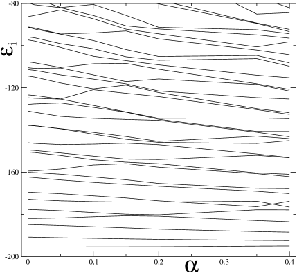
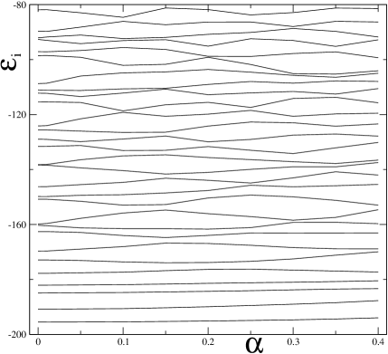
Figure 2: The same s.p. spectrum of levels as in Fig. 1 but with the projection of the angular momentum $m=0$.

Figs 1 and 2 show two examples for the full spectra of the s.p. energies $\varepsilon_{i}$ and for the fixed angular momentum projection $m=0$ versus the deformation parameter $\alpha$ for the $P_{2}$ and $P_{5}$ shapes, respectively. The spectra for $P_{3}$ and $P_{4}$ are very similar to the $P_{5}$ case and therefore, they are not shown. As seen from Fig. 1, there are clear shell effects in the full spectra at small deformations, approximately at $\alpha\;\hbox{\kern 1.00006pt\lower 3.01385pt\hbox{$\sim$} \kern-11.19997pt\raise 2.15277pt\hbox{$<$} \kern 1.00006pt}0.1$ for all multipolarities from the $P_{2}$ shape to the $P_{5}$ one. With increasing deformation $\alpha$, the shell gaps become less pronounced and slowly changed in the region $\alpha\approx 0.1-0.4$ for all these multipolarities. Much more differences can be found in comparison of Fig. 1 for full spectra and Fig. 2 for $m=0$ levels only. The shell effects are seen here too but much less pronounced. The spectrum of levels with $m=0$ becomes more uniform with increasing multipolarity $n$.

The key quantity for calculations of the NNSD $P(S)$ is the level density $g(\varepsilon)$, see Appendix A and Refs wigner ; porter ; brody ; aberg ; mehta . For these calculations one may apply the Strutinsky shell correction method writing

$$g_{\Gamma}(\varepsilon)=\tilde{g}(\varepsilon)+\delta g_{\Gamma}(\varepsilon).$$ (4)

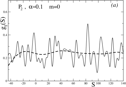
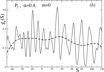
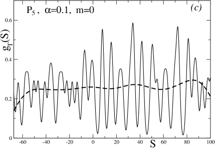
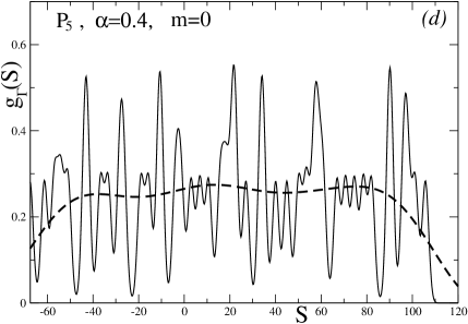
Figure 4: The same as in Fig. 3 but for levels with the fixed projection of the angular momentum $m=0$.

The smooth part $\tilde{g}(\varepsilon)$ is defined by the Strutinsky smoothing procedure strut ; FH . The so called plateau condition (stability of values of the smooth level density $\tilde{g}$ as function of the averaging parameters: Gaussian width $\Gamma$ and the degree of the correction polynomial $M$ takes place at $\Gamma=20-40$ MeV and $M=4-8$). Figs 3 and 4 for full spectra and for fixed angular momentum projection $m=0$ show the typical examples of the level densities (smooth component and the total density with the oscillating part) for the same degree of the Legendre polynomials $n=2$ and $5$ at deformations $\alpha=0.1$ and $0.4$, in correspondence with spectra presented in Figs 1 and 2, respectively. In Fig. 4 for the case of the specific $m=0$ levels, one has somewhat larger Gaussian width parameters of the smooth level density $\tilde{g}$ in the total density (Eq. (4)) than those for the full spectra in Fig. 3. As seen clearly from Figs 3 and 4 the smooth level density for the $m=0$ spectra is more flat (besides of relatively small remaining oscillations because of much less levels with the fixed $m=0$), as compared to the full-spectra results. This more flat behavior for the fixed $m$ value is due to the loss of the symmetry. Therefore one expects the system with the fixed angular momentum $m$ to be more chaotic. The differences between Fig. 3 and Fig. 4 are quite remarkable. On the other hand differences between pictures within Fig. 3 or Fig. 4 are less notable and as one can see shell effects are still remaining at bigger deformations and multipolarities.

III NEAREST-NEIGHBOR SPACING DISTRIBUTIONS

Following the review paper brody , the distribution ${\cal P}(S)$ for the probability of finding the spacing $S$ between the nearest neighboring levels is given by (see also Refs wigner ; porter ; aberg ; mehta and Appendix A)

$${\cal P}(S)=g(S)\;\exp\left(-\int_{0}^{S}g(x)\;\mbox{d}x\right)/\aleph.$$ (5)

The key quantity $g(S)$ can be considered as the density of the s.p. levels counted from a given energy, say, the Fermi energy $E_{F}$. $D$ is a mean uniform distance between neighboring levels so that $1/D$ is the mean density of levels. $\aleph$ is the normalization factor for large enough maximal value of $S$, $S_{max}$,

$$\aleph=\int_{0}^{S_{max}}\mbox{d}xg(x)\;exp\left(-\int_{0}^{x}g(y)\mbox{d}y\right)/D.$$ (6)

This normalization factor $\aleph$ can be found from the normalization conditions:

$$\int\mbox{d}x{\cal P}(x)=\int\mbox{d}xx{\cal P}(x)=1\;.$$ (7)

[Notice that for convenience we introduced the dimensionless probability ${\cal P}$ in contrast to that of Ref. brody denoted as $P(S)$, see Eq. (1.3) there.]

The Poisson law follows if we take constant for the level density, $g(S)=1/D$, in Eq. (5),

$${\cal P}(S)=\exp\left(-S/D\right)\;.$$ (8)

Wigner’s law follows from the assumption of the linear level density, proportional to $S$,

$${\cal P}(S)=\left(\pi S/2D\right)\;\exp\left(-\pi S^{2}/4D^{2}\right)\;.$$ (9)

Both distributions are normalized to one for large enough maximal value of $S$, $S_{max}=\infty$ to satisfy Eq. (7).

The level density in fact is not a constant or $\propto S$. The combination of the Poisson and Wigner distributions was suggested in Ref. berrob by introducing one parameter. For our purpose to keep a link with the properties of the level density, like smooth and shell components strut , it is convenient to define the probability ${\cal P}(S)$ (Eq. (5)) for a general linear level-density function through two parameters ${\cal A}$ and ${\cal B}$,

$$g(S)=\left({\cal A}+{\cal B}S/D\right)/D\;.$$ (10)

Substituting Eq. (10) into the general formula (Eq. (5)) one obtains explicitly the analytical result in terms of the standard error functions, $\mbox{erf}(z)=2\int_{0}^{z}\mbox{d}x\;\exp(-x^{2})/\sqrt{\pi}$,

$${\cal P}(S)=\left(1+{\cal B}\xi/{\cal A}\right)\;\exp\left(-{\cal B}\xi^{2}/2-{\cal A}\xi\right)/\left[\aleph_{0}+{\cal B}\;\aleph_{1}/{\cal A}\right]\,,$$ (11)

$$\aleph_{0} = \int_{0}^{\cal C}\mbox{d}\xi\;\exp\left(-\frac{{\cal B}}{2}\xi^{2}-{\cal A}\xi\right)=\sqrt{\frac{\pi}{2{\cal B}}}\;\exp\left(\frac{{\cal A}^{2}}{2{\cal B}^{2}}\right)\;\mbox{erf}\left(\frac{{\cal A}+{\cal B}{\cal C}}{\sqrt{2{\cal B}}}\right),$$

$$\aleph_{1} = \int_{0}^{\cal C}\mbox{d}\xi\xi\;\exp\left(-\frac{{\cal B}}{2}\xi^{2}-{\cal A}\xi\right)=-\frac{1}{{\cal B}}\left[\exp\left(-\frac{{\cal B}}{2}{\cal C}^{2}-{\cal A}{\cal C}\right)+{\cal A}\;\aleph_{0}\right].$$ (12)

where $\xi=S/D$, ${\cal C}=S_{max}/D$ is the maximal value of $\xi$. For large ${\cal C}\rightarrow\infty$ one has simply $\aleph_{0}\rightarrow\sqrt{\pi/2{\cal B}}\;\exp\left({\cal A}^{2}/2{\cal B}^{2}\right)$ and $\aleph_{1}\rightarrow-{\cal A}\aleph_{0}/{\cal B}$. Taking the limits ${\cal A}\rightarrow 1$, ${\cal B}\rightarrow 0$ and ${\cal A}\rightarrow 0$, ${\cal B}\rightarrow 1$ in (11) one simply finds exactly the standard Poisson (Eq. (8)) and Wigner (Eq. (9)) distributions. In this way the constants ${\cal A}$ and ${\cal B}$ are measures of the probability to have Poisson and Wigner distributions (Eq. (10)).

IV NUMERICAL RESULTS

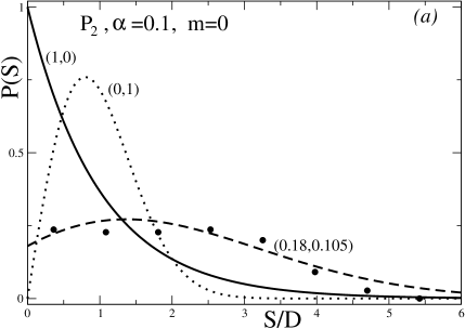
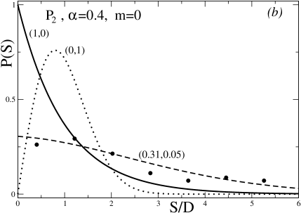
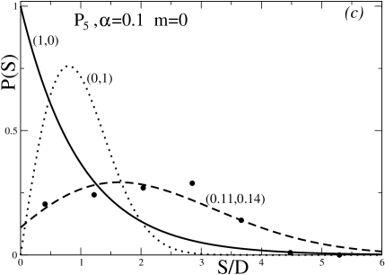
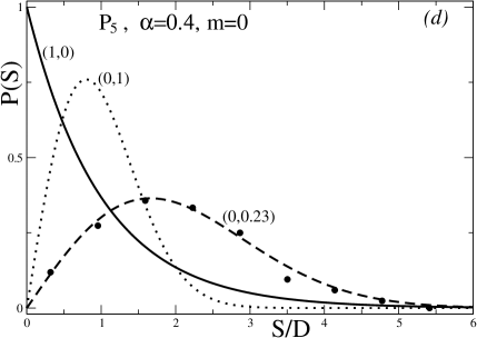
Figure 6: The same as in Fig. 5 but for the spectra of Figs 2, 4.

Figs 5 and 6 show the corresponding NNSD $P(S)$ (Eq. (5)). Again, in accordance with spectra (see Figs 1, 2) and level-density calculations in Figs 3 and 4, the dramatic changes are observed between Fig. 6 for the NNSD $P(S)$ with the $m=0$ and Fig. 5 for those of the full spectra ones. Results presented by heavy dots in Fig. 5 look more close to the Poisson distribution and those in Fig. 6 are more close to the Wigner one.

There are a large difference in numbers ${\cal A}$ and ${\cal B}$ which measure the closeness of the distributions $P(S)$ for the neighboring levels spacing to the standard ones, Poisson (1,0) and Wigner (0,1). However, in Fig. 6 all distributions are more close to the Wigner in shape having a maximum between zero and large compared to $D$ value $S_{max}$ with respect to $D$ [ $S_{max}={\cal C}D$, see immediately after Eq. (12)] than monotonous exponential-like decrease similar to the Poisson behavior in Fig. 5. Notice that we have more pronounced Wigner-like distribution with increasing multipolarity $n$ and deformation $\alpha$ in Fig. 6, especially remarkable at $P_{5}$ surface distortions and large enough deformation $\alpha=0.4$, see last plot $(d)$ in Fig. 6. Including all the angular momentum projections $m$ for all desired multipolarities and deformations one has clearly Poisson-like behavior though they differ essentially in numbers ${\cal A},{\cal B}$ from the standard ones (1,0), see Fig. 6.

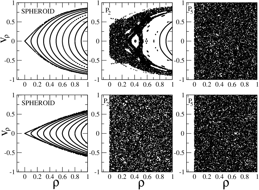
Figure 7: Poincare sections $v_{\rho}$ vs $\rho$ for spheroid, $P_{2}$ and $P_{5}$ shapes at the small deformation $\alpha=0.1$ (upper row) and large deformation $\alpha=0.4$ (lower row) for the projections of the angular momentum on the symmetry axis $m=0$.

The reason for this can be understood looking at the Poincare sections shown in Fig. 7 arvieu ; blshsw ; kiev2010 . The upper row is related to a small deformation and lower row corresponds to a large deformation. The projection of the angular momentum is $m=0$ in all pictures of Fig. 7. Difference is remarkable for the integrable spheroidal cavity and other non-integrable (in the plane of the symmetry axis) shapes. As seen from comparison of upper and lower plot lines, with increasing deformation $\alpha$ and multipolarity $n$ we find more chaotic behavior and we should expect therefore the NNSD closer to the Wigner distribution (9). This is in agreement with the NNSD calculations for the fixed $m=0$, see Fig. 6. Notice that similar properties of the NNSD for other potentials and constraints were discussed in Refs heiss1 ; heiss3 ; nazm1 ; nazm2 .

The difference between the NNSD calculations with the realistic level densities by the Strutinsky shell-correction method (see Eq. (4)) for the considered WS potential and those with their idealistic linear behavior (Eq. (10)) can be studied in terms of the general formula $P(S)$ (Eq. (5)). In particular, the shell effects related to the inhomogeneity of the s.p. levels near the Fermi surface for all desired multipolarities and deformations are found to be significant, also in relation to the fixed quantum number $m$.

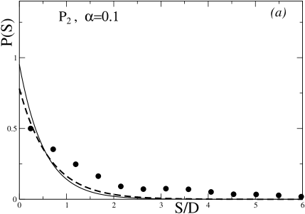
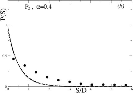
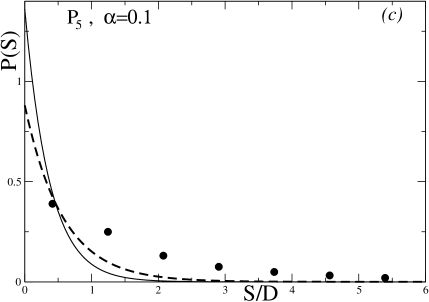
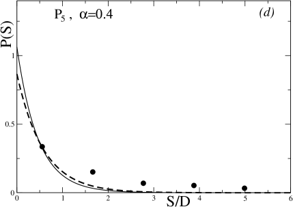
Figure 8: The general distribution $P(S)$ (Eq. (5)) vs the energies $S$ for the same spectra as in Figs 1, 3, 5; dashed are the distributions $P(S)$ related to the Strutinsky smooth density $\tilde{g}(S)$ and solid is the total level density $g_{\Gamma}(S)$ (Eq. (4)); dots are the same as in Figs 5 and 6.

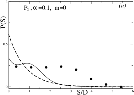
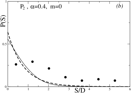
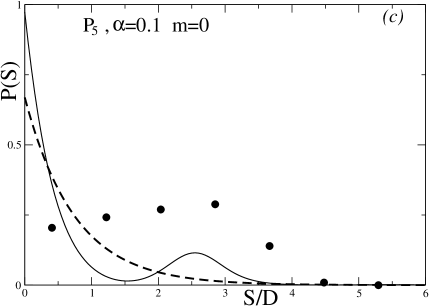
Figure 9: The same as in Fig. 8 but for spectra of Figs 2, 4 and 6.

Figs 8 and 9 show the results of these calculations corresponding to Figs 5 and 6. Notice that in the case of the full spectra, see Fig. 8, one has Poisson-like distributions corresponding to the smooth density (dashed) with a similar behavior as NNSD shown by heavy dots, in contrast to Fig. 9 where we find rather big differences between these curves. The shell effects are measured by the differences between the solid curve related to the total level density with the shell components and the dashed one for the smooth level density of Figs 3 (all $m$) and 4 (with $m=0$), see correspondingly Figs 8 and 9. With increasing deformations one has slightly decreasing the shell effects, in contrast to the multipolarity dependence for which there is almost no change of the shell effects at the same deformations.

V CONCLUSIONS

We studied the statistics of the neighboring s.p. levels in the WS potential for several typical multipolarities and deformations of the surface shapes and deformations, as compared with the standard Poisson and Wigner distributions $P(S)$. For the sake of comparison, we derived analytically the combine asymptotic Poisson-Wigner distribution $P(S)$ related to the general linear dependence of the corresponding s.p. level density. We found the significant differences between distributions for a fixed value of the angular momentum projection $m$ of the particle and those accounting all possible values of $m$. For the case of the fixed $m=0$ we obtained distributions $P(S)$ more close to the Wigner shape with the maximum between $S=0$ and a maximal large value of $S$, the more pronounced the larger multipolarity and deformation of the potential surface. We found also that the full spectra distributions $P(S)$ look Poisson-like in a sense that they have maximum at $S=0$ and almost exponential decrease as a function of the energy near the Fermi surface. Our results clarify the widely extended opinion of the relation of the distributions (Poisson or Wigner) to the integrability of the problem (the integrable or chaotic one). All considered potentials are axially-symmetric but they are the same non-integrable ones in the plane of the symmetry axis. However, the degree of the symmetry (classical degeneracy myab ; strutmag ; smod ${\cal K}$, i.e. the number of the single-valued integrals of motion besides of the energy) for the case of the full spectra, Figs 1, 3, 5, ( ${\cal K}=1$, a mixed system) is higher than for the fixed angular momentum $m$ (${\cal K}=0$ like for the completely chaotic system). Notice that integrability is not only one criterium of chaoticity. The measure of the differences of the distributions $P(S)$ between Poisson and Wigner standard ones depends also on the properties of the energy dependence of the level density (from constant to proportional-to-energy dependence). From comparison between the general distribution $P(S)$ related to the smooth level density obtained by the Strutinsky shell correction method and the statistics of the neighboring s.p. levels one finds that all of them are more close to the Poisson-like behavior. This shows that the energy dependence of the smooth level density differs much from the linear functions. We obtained also large shell effects in the distributions $P(S)$ in nice agreement with those in the key quantity in this analysis, - level density dependencies on the energy near the Fermi surface.

As to perspectives, it might be necessary to use the combined microscopic-macroscopic approaches myersswiat ; strut to clear up the results more systematically and analytically. Our quantum results can be interesting for understanding the one-body dissipation at slow and faster collective dynamics with different shapes like the ones met in nuclear fission and heavy-ion collisions.

VI Acknowledgements

We thank S. Aberg, V.A. Plujko and S.V. Radionov for valuable discussions.

Appendix A: A derivation of the NNSD

We introduce first the level density, $g(E)$, as the number of the levels ${\mbox{d}}N$ in the energy interval [$E,E+{\mbox{d}}E$] divided by the energy interval, $g(E)={\mbox{d}}N/{\mbox{d}}E$. With the help of this quantity one can derive the NNSD $P(S)$ as the probability density versus the spacing $S$ between the nearest neighboring levels. Specifying $P(S)$ to the problem with the known s.p. spectra of the Hamiltonian, one can split the energy interval $\Delta E$ under the investigation into many small (equivalent for simplicity) parts $\Delta S\ll\Delta E$. Each of $\Delta S$ nevertheless contain many energy levels, $\Delta S\gg D$. Then, we find the number of the levels which occur inside of the small interval $\Delta S$. Normalizing these numbers by the total number of the levels inside the total energy interval $\Delta E$ one obtains the distribution which we shall call as the probability density $P(S)$. Notice that the result of this calculation depends on the energy length of the selected $\Delta S$. In our calculations, we select $\Delta S$ by the condition of a sufficient smoothness of the distribution $P(S)$. Such procedure is often used for the statistical treatment of the experimentally obtained spectrum with the fixed quantum numbers like the angular momentum, parity and so on brody .

Following mainly Ref. aberg , let us calculate first the intermediate quantity $f(S)$ as the probability that there is no energy level in the energy interval [$E,E+S$]. According to the general definition of the level density mentioned above, $g(S){\mbox{d}}S$ can be considered as the probability that there is one energy level in $[E+S,E+S+{\mbox{d}}S]$. Then,

$$f(S+{\mbox{d}}S)=f(S)\left(1-g(S){\mbox{d}}S\right)\;,$$ (A1)

which leads to the differential equation for $f(S)$,

$${\mbox{d}}f=-g(S){\mbox{d}}Sf(S).$$ (A2)

Solving this equation one gets

$$f(S)=C\exp\left(-\int_{0}^{S}g(x){\mbox{d}}x\right)\;.$$ (A3)

Let $P(S)\mbox{d}S$ denote the probability that the next energy level is in $[E+S,E+S+\mbox{d}S]$,

$$P(S){\mbox{d}}S=f(S)g(S){\mbox{d}}S\;.$$ (A4)

Then, substituting Eq. (A3) into Eq. (A4) one finally arrives at the general distribution:

$$P(S)=Cg(S)\exp\left(-\int_{0}^{S}g(S^{\prime}){\mbox{d}}S^{\prime}\right).$$ (A5)

The boundary conditions in solving the differential equation (A2) accounts for the meaning of the NNSD $P(S)$ and its argument as the spacing between the nearest neighbor levels as shown in the integration limit in Eq. (A5). The constant $C$ is determined from the normalization conditions (Eq. (6)).

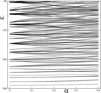
Figure 1: The s.p. energy levels $\varepsilon_{i}$ in the WS potential ($V_{0}=200$ MeV, $R_{0}=6.622$ fm, $a=0.1$ fm) as function of the deformation $\alpha$ for the $P_{2}$ (left) and $P_{5}$ (right) shapes (Eq. (3)).

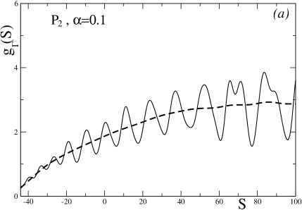
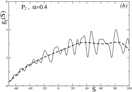
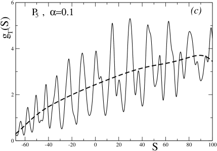
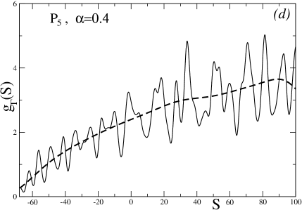
Figure 3: The level densities $g_{\Gamma}(S)$ (Eq. (4)) as a function of the energy counted from the Fermi level ($S=0$) for a given particle number $N$ for spectra of the s.p. levels of Fig. 1 for the $P_{2}$ $(a,b)$ and $P_{5}$ $(c,d)$ shapes at the small $\alpha=0.1$ (left, $a,c$) and larger $\alpha=0.4$ (right,$b,d$) deformations; dashed is the smooth density $\tilde{g}(S)$ (Eq. (4)); solid is the total density $g_{\Gamma}(S)$ (Eq. (4)) ($\Gamma=3$ MeV, $M=0$ for $\delta g_{\Gamma}(S)$).

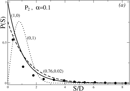
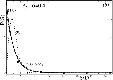
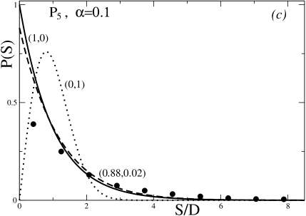
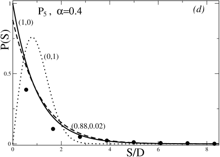
Figure 5: The distributions of spacing of the neighboring levels $P(S)$ represented by heavy dots brody vs the energies $S$ for the same spectra as in Figs 1 and 3. Solid curve is a standard Poisson distribution (Eq. (8)) and a dotted one is a standard Wigner distribution (9). Numbers in brackets $({\cal A},{\cal B})$ show ${\cal A}$ and ${\cal B}$ of Eq. (11). Dashed curve corresponds to a linear approximation to the level density (Eq. (10)); other notations are the same as in Figs 3 and 4.

References

- (1) E.P. Wigner, Proc. Cambridge Philos. Soc. 47, 790 (1951); Canadian Math. Congress Proceedings, University of Toronto Press, Toronto, Canada, 174 (1957); ibid. SIAM Rev. 9, 1 (1967).
- (2) C.E. Porter, Statistical theories of spectra: fluctuations, Academy Press, New York (1965).
- (3) T.A. Brody et al., Rev. Mod., 53, 385 (1981).
- (4) M.L. Mehta, Random Matrices, Academic Press, San Diego, New York, Boston, London, Sydney, Tokyo, Toronto (1991).
- (5) S. Aberg, Quantum Chaos, (Mathematical Physics, Lund, Sweden, 2002).
- (6) W.D. Myers and W.J. Swiatecki, Nucl. Phys. 81, 1 (1966); ibid. Ann. Phys. (N.Y.) 55, 395 (1969).
- (7) V.M. Strutinsky, Nucl. Phys. A 95, 420 (1967); ibid. 122, 1 (1968).
- (8) J. Blocki, Y. Boneh, J.R. Nix, J. Randrup, M. Robel, A.J. Sierk, and W.J. Swiatecki, Ann. Phys. (N.Y.) 113, 330 (1978).
- (9) J. Blocki, J. Skalski, W.J. Swiatecki, Nucl. Phys. B 594, 137 (1995).
- (10) J. Blocki, J.-J. Shi and W.J. Swiatecki, Nucl. Phys. A 554, 387 (1993).
- (11) J. Blocki, J. Skalski, W.J. Swiatecki, Nucl. Phys. A 618, 1 (1997).
- (12) C. Jarzynski and W.J. Swiatecki, Nucl. Phys. A 552, 1 (1993).
- (13) P. Magierski, J. Skalski and J. Blocki, Phys. Rev. C 56, 1011 (1997).
- (14) J.P. Blocki, A.G. Magner, and I.S. Yatsyshyn, At. Nucl. and Energy, 11, 239 (2010); ibid Int. J. Mod. Phys. E 20, 292 (2011).
- (15) S.E. Koonin and J. Randrup, Nucl. Phys. A 289, 475 (1977).
- (16) A.G. Magner, A.M. Gzhebinsky, S.N. Fedotkin, Phys. Atom. Nucl. 70, 647 (2007); ibid 70, 1859 (2007).
- (17) A.M, Gzhebinsky, A.G. Magner, and S.N. Fedotkin, Phys. Rev. C 76, 064315 (2007).
- (18) R. Arvieu, F. Brut, J. Carbonell, and J. Touchard, Phys. Rev. A 35, 2389 (1987); ibid. Nucl. Phys. A 545, C497 (1992).
- (19) W.D. Heiss, R.G. Nazmitdinov, and S. Radu, Phys. Rev. Lett. 72, 2351 (1994).
- (20) W.D. Heiss and R.G. Nazmitdinov, Phys. Rev. Lett. 73, 1235 (1994).
- (21) M. Brack et al., Rev. Mod. Phys., 44, 320 (1972).
- (22) A.G. Magner, I.S. Yatsyshyn, K. Arita, and M. Brack, Phys. Atom. Nucl., 74, 1475 (2011).
- (23) W.D. Heiss, R.G. Nazmitdinov, and S. Radu, Phys.Rev. C 52, 3032 (1995).
- (24) W.D. Heiss and R.G. Nazmitdinov, Physica D, 118, 134 (1998).
- (25) A. Hamoudi, R.G. Nazmitdinov, E. Shahaliev, and Y. Alhassid, Phys. Rev. C 65, 064311 (2002).
- (26) R.G. Nazmitdinov, E.I. Shahaliev, M.K. Suleymanov, and S. Tomsovic, Phys. Rev. C 79, 054905 (2009).
- (27) V.M. Strutinsky and A.G. Magner, Sov. Phys. Part. Nucl., 7, 138 (1976).
- (28) V.M. Strutinsky, A.G. Magner, S.R. Ofengenden, and T. Døssing, Z. Phys. A 283, 269 (1977).
- (29) M. Brack and R.K. Bhaduri, Semiclassical Physics. Frontiers in Physics, 96, Addison-Wesley, Reading, MA. (1997); 2nd edition, Westview Press, Boulder (2003).
- (30) M. Gutzwiller, J. Math. Phys. 12, 343 (1971); Chaos in Classical and Quantum Mechanics, Springer-Verlag, N.Y. (1990).
- (31) M.V. Berry and M. Robnik, J. Phys. A 17, 2413 (1984).