Superluminal Tachyonlike Excitations of Dirac Fermions in a Topological Insulator Junction

Abstract

We have considered a system of two topological insulators and have determined the properties of the surface states at the junction. Here we report that these states, under certain conditions exhibit superluminous (tachyonic) dispersion of the Dirac fermions. Although superluminal excitations are known to exist in optical systems, this is the first demonstration of possible tachyonic excitations in a purely electronic system. The first ever signature of tachyons could therefore be found experimentally in a topological insulator junction.

Topological insulators (TIs), a new class of materials rich with new concepts and promises, have attracted considerable attention in the condensed matter physics community topo_review . In the bulk, the system is electrically insulating, driven by the strong spin-orbit coupling present in the system. The three-dimensional (3D) TIs host a single Dirac cone in the surface states that was confirmed experimentally by angle-resolved photoemission spectroscopy. Dirac fermions are also present in graphene abergeletal . However, in the TIs, unlike in graphene, there exists only odd number of non-degenerate Dirac cones with spin-momentum locking that results in helical Dirac fermions helical without spin degeneracy. This spin chirality of Dirac fermions prevents them from backscattering and localization roushan . That makes those systems ideal for spintronics applications or for quantum computing topo_review . Until now, most of the attentions have been heaped on the surface states of a single TI. Here we show that, the junction surface states of two TIs, in certain situations, exhibit superluminal (tachyonic) dispersion of Dirac fermions. Tachyons have eluded detection until now, despite diligent efforts by the particle physicists worldwide. However, as we have demonstrated below, it could perhaps be found in the present solid state system.

We consider a junction between two topological insulators. The junction surface is described by $z=0$, and we assume that the system of TIs is isotropic in $x$ and $y$ directions. Therefore, the surface states are characterized by the $x$ and $y$ components of the wave vector, $k_{x}$ and $k_{y}$, and the surface wave functions depend on the $z$-coordinate and decay in both directions, i.e., the positive and negative directions of the $z$ axis [see inset in Fig. 1(b)]. We label the topological insulator at $z<0$ as TI-1, and the topological insulator at $z>0$ as TI-2. We have found that for a general variation of parameters of TI-2, the junction surface states exhibit one branch with unique tachyonic dispersion relation. Although, they are not yet found experimentally, these “Überlichtgeschwindigkeitteilchen” (faster than light particles) discussed by Sommerfeld sommer in 1905, and many others tachyonics since then, have always been vigorously pursued (e.g., in the case of the neutrinos chodos ; ehrlich ) by the particle physics community for many decades foundation .

We assume that the electronic states of both TIs are described by the same type of low-energy effective 3D Hamiltonian liu_2010 ; zhang_2009 , which has the $4\times 4$ matrix form and can be expressed as

$${\cal H}_{\rm TI}=\varepsilon(\vec{k})+\left(\begin{array}[]{cc}M(\vec{k})\sigma_{z}-{\rm i}A_{1}\sigma_{x}\partial_{z}&A_{2}k_{-}\sigma_{x}\\ A_{2}k_{+}\sigma_{x}&M(\vec{k})\sigma_{z}+{\rm i}A_{1}\sigma_{x}\partial_{z}\end{array}\right),$$ (1)

where $\sigma_{i}$ ($i=x,y,z$) are the Pauli matrices, $\partial_{z}=\partial/\partial z$, $\vec{k}=(k_{x},k_{y})$ is a two-dimensional (2D) wave vector, $k_{\pm}=k_{x}\pm{\rm i}k_{y}$, and

$$\varepsilon(\vec{k})=C_{1}-D_{1}\partial_{z}^{2}+D_{2}(k_{x}^{2}+k_{y}^{2}),$$ (2)

$$M(\vec{k})=M_{0}+B_{1}\partial_{z}^{2}-B_{2}(k_{x}^{2}+k_{y}^{2}).$$ (3)

For a topological insulator of the type $\mbox{Bi}_{2}\mbox{Se}_{3}$, the four-component wave functions, $\Psi$, corresponding to the matrix Hamiltonian (1) determine the amplitudes of the wave functions at the positions of Bi and Se atoms: $(\mbox{Bi}_{\uparrow},\mbox{Se}_{\uparrow},\mbox{Bi}_{\downarrow},\mbox{Se}_{\downarrow})$, where the arrows indicate the direction of the electron spin. In the case of $\mbox{Bi}_{2}\mbox{Se}_{3}$ TI, the constants in the Hamiltonian (1) are zhang_2009 , $A_{1}=2.2$ eV$\cdot$Å, $A_{2}=4.1$ eV$\cdot$Å, $B_{1}=10$ eV$\cdot$Ų, $B_{2}=56.6$ eV$\cdot$Ų, $C_{1}=-0.0068$ eV, $D_{1}=1.3$ eV$\cdot$Ų, $D_{2}=19.6$ eV$\cdot$Ų, and $M_{0}=0.28$ eV.

The unique properties of the bulk Hamiltonian (1) is that, for a single TI, it can produce surface states with massless relativistic dispersion relation, $E\approx v_{\rm F}k$, where $v_{\rm F}=A_{2}\sqrt{1-(D_{1}/B_{1})^{2}}$ shan_2010 is the Fermi velocity. In the case of two TIs, at the junction we expect a coupling between two surface states belonging to different TIs. Within a simple model which includes phenomenological coupling between massless relativistic states of the two TIs, it was shown earlier that the properties of the junction surface states strongly depend on the relative sign of the Fermi velocities of the two TIs, i.e., on the relative sign of $A_{2}$ for TI-1 and TI-2 takahashi . Here we show that for a realistic 3D model [Eq. (1)] of the TI, one can observe new and unique features in the dispersion relation of the junction states.

In what follows, we study the junction surface states within the realistic 3D model of the TI. For two TIs, we assume that both TIs are described by the Hamiltonian of the same type (1) but with different constants. To distinguish the constants corresponding to different TIs, we introduce superscripts $(1)$ and $(2)$ for TI-1 and TI-2, respectively. Following the general procedure of constructing the surface states of a TI shan_2010 ; zhou_2008 , we first determine for each TI the general bulk solution of the Schrödinger equation of the form $\Psi\propto{\rm e}^{\lambda^{(m)}z}\,{\rm e}^{{\rm i}\vec{k}\vec{\rho}}$, where $m=1$ and 2 for TI-1 and TI-2, respectively. Substituting this form of solution in the Schrödinger equation, ${\cal{H}}_{\rm TI}(\vec{k},\partial_{z})\Psi=E\Psi$, we obtain a secular equation, $\det\left[{\cal{H}}^{(m)}_{\rm TI}(\vec{k},\lambda^{(m)})-E\right]=0$, for each TI ($m=1,2$). For each energy $E$, this equation defines four values of $\lambda^{(m)}_{\alpha}(k,E)$, $\alpha=1,\ldots,4$. Each $\lambda^{(m)}_{\alpha}(k,E)$ is doubly degenerate, which finally generates eight wave functions for each TI, $m=1$ and 2, $\Psi^{(m)}_{s,\alpha}(k,E)\,{\rm e}^{\lambda^{(m)}_{\alpha}z}{\rm e}^{{\rm i}\vec{k}\vec{\rho}}$ (see Ref. shan_2010 ; zhou_2008 ), where $s=1,2$, $\alpha=1,\ldots,4$, and $\Psi^{(m)}_{s,\alpha}(k,E)$ is a four-component wave function.

Our goal here is to determine the surface states localized at the junction of the two TIs. Therefore, out of the four values of $\lambda^{(m)}$ (for each TI), we choose only two values: for TI-1 ($z<0$) with $\mbox{Re}\lambda^{(m)}_{\alpha}>0$ and for TI-2 ($z>0$) with $\mbox{Re}\lambda^{(m)}_{\alpha}<0$. After selection of these $\lambda^{(m)}_{\alpha}$ ($\alpha=1,2$), our junction surface states then take the form

$$\Phi(\vec{\rho},z)=\left\{\begin{array}[]{l}\sum\limits_{{s=1,2}\atop{\alpha=1,2}}C^{(1)}_{s,\alpha}\Psi^{(1)}_{s,\alpha}\,{\rm e}^{\lambda^{(1)}_{\alpha}z}{\rm e}^{{\rm i}\vec{k}\vec{\rho}},z<0\\ \sum\limits_{{s=1,2}\atop{\alpha=1,2}}C^{(2)}_{s,\alpha}\Psi^{(2)}_{s,\alpha}{\rm e}^{\lambda^{(2)}_{\alpha}z}\,{\rm e}^{{\rm i}\vec{k}\vec{\rho}},z>0.\end{array}\right.$$ (4)

This type of wave function determines the localized junction surface states. The energy of the junction state is found from the condition of continuity of the wave function, $\Phi(z)$, and the corresponding current, $[\delta{\cal H}^{(m)}_{\rm TI}/\delta k_{z}]\Phi(z),\ (k_{z}={\rm i}\partial_{z}$) at the junction between the two TIs. Solution of this continuity equations determines the dispersion relation, $E(k)$, of the junction surface states.

Figure 1: (a) Dispersion relation of the junction states. The parameters of the TI-2 are the same as the parameters of TI-1 except for $A^{(2)}_{1}=2.2$ eV$\cdot$Å. Near the point B the dispersion relation shows the tachyonic behavior with superluminal group velocity. (b) The localization length of the junction states shown in panel (a). Near the tachyonic point (point B) the junction states are strongly localized with localization length $\approx 10$ Å. At the edge of the tachyonic branch (near points A and C) the states become delocalized. Inset: Schematic illustration of the junction (red line) between two TIs. The coordinate system is introduced as follows: $z$-axis is perpendicular to the junction surface, and $x$ and $y$ are in the plane of the junction.

We keep the parameters of TI-1 fixed as for $\mbox{Bi}_{2}\mbox{Se}_{3}$ (as given above) and vary the parameters of TI-2. Our results indicate that for general variation of the parameters of TI-2, the junction surface states show one branch with unique dispersion relation that resembles the dispersion of the tachyons chiao96 . In Fig. 1 we show the dispersion relation for the junction state when only one parameter, $A_{1}$, of TI-2 is different from TI-1. In this case there is only one type (tachyonic) of dispersion. The group velocity, $v_{g}=\partial E(k)/\partial k$, corresponding to the tachyonic dispersion becomes infinitely large at $k\approx k_{0}$ [point B in Fig. 1(a)]. Similar superluminal dispersion was known to be present (theoretically) for propagation of the optical pulses through inverted two-level system of atoms chiao96 and in metamaterial photonic crystals chen11 with folded bands. Superluminal propagation can also be observed for propagation of light pulses through a media with anomalous dispersion relation milonni02 . In all these cases, the tachyonic dispersion is achieved for propagation of light pulses through a specially designed medium. In contrast, our system consists of just electronic degrees of freedom and propagation of electronic excitations exhibits tachyonic dispersion. If confirmed experimentally, this would be the first example of superluminal tachyonic dispersion in an actual semiconductor (electronic) system.

In Fig. 1(b) we show the localization length in the $z$-direction of the junction states of the tachyonic branch. The localization length is defined as $l_{z}=\mbox{min}\left\{1/|\mbox{Re}\lambda^{(m)}_{s,\alpha}|\right\}$. Clearly, the maximum localization of the surface states occur near the tachyonic point B with localization length $\approx 10$ Å. These strongly localized states are less sensitive to the bulk disorder of the TIs, which can help with the experimental observation of the tachyonic states. Away from the tachyonic point the junction states become weakly localized and finally, near the ends of the tachyonic branch (points A and C) the junction states become delocalized. The actual distribution of electronic density for the two (up and down) spin components, is shown in Fig. 2 for one of the junction states near point B [see Fig. 1(a)]. Both spin components are occupied with final non-zero spin-polazition of the junction tachyonic states. Exactly at the tachyonic point the junction state is spin unpolarized.

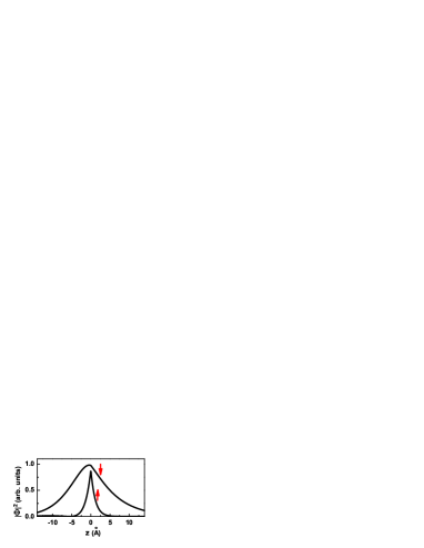
Figure 2: The electron density along the $z$ direction for the tachyonic branch shown in Fig. 1(a). The density is shown for the junction surface state at $k=0.084$ Å^-1. The arrows next to the lines are the directions of the electron spin. The junction between the TIs is at $z=0$.

The existence of a tachyonic branch in the dispersion relation of junction states means that the energy dispersion becomes a non-analytic function of the 2D surface momentum, i.e., the group velocity $v_{g}=\hbar^{-1}\partial E(k)/\partial k$ is infinitely large. Due to the analytical dependence of the Hamiltonian (1) on the wave vector $\vec{k}$, the non-analyticity in the dispersion relation is possible only if the Hamiltonian is non-hermitian. In our case the junction states are decaying states, i.e., $\Phi\propto{\rm e}^{\lambda_{\alpha}z}$, where the real part of $\lambda_{\alpha}$ is non-zero. For these states the Hamiltonian becomes non-hermitian and tachyonic branches are therefore allowed. The existence of tachyonic dispersion does not violate Einstein’s causality principle. The reason is that the superluminal group velocity describes the propagation of not a signal but an analytical wave packet. The propagation of a singularity, i.e., the signal, is not described by the group velocity, so there is no violation of Einstein’s causality relation (see Ref. chiao96 ; milonni02 ).

The tachyonic excitations can be described by an effective 2D Hamiltonian. This effective Hamiltonian should have a $2\times 2$ matrix form, which takes into account the electron spin degrees of freedom. In addition, the Hamiltonian should also support the non-analytical tachyonic dispersion relation and should be non-hermitian. The tachyonic Hamiltonian can be constructed, for example, by introducing the imaginary proper mass in the Dirac equation jentschura12 . In our case, the tachyonic Hamiltonian is achieved by introducing an imaginary Fermi velocity in the massive Dirac equation. More precisely, the effective Hamiltonian which describes the tachyonic junction surface states has the form

$${\cal H}_{\mbox{Tach}}=\left(\begin{array}[]{cc}\Delta_{0}&{\rm i}\hbar v_{\rm I}k_{+}\\ {\rm i}\hbar v_{\rm I}k_{-}&-\Delta_{0}\end{array}\right)=\Delta_{0}\sigma_{z}+{\rm i}\hbar v_{\rm I}(\vec{\sigma}\vec{k}),$$ (5)

where $\Delta_{0}$ is the effective mass of the tachyons, and ${\rm i}v_{\rm I}$ is the imaginary Fermi velocity. This effective Hamiltonian produces a tachyonic branch with dispersion relation of the form

$$E_{\mbox{Tach}}(k)=\pm\sqrt{\Delta_{0}^{2}-\hbar^{2}v_{\rm I}^{2}k^{2}}.$$ (6)

Therefore, $k<k_{0}=\Delta_{0}/\hbar v_{\rm I}$ and the group velocity at $k=k_{0}$ becomes infinitely large. For the tachyonic branch shown in Fig. 1 the parameters of the effective Hamiltonian (5) are $\Delta_{0}=0.313$ eV and $v_{\rm I}=5.7\times 10^{5}$ m/s.

The wave function corresponding to Hamiltonian (5) with energy spectrum (6) has the following form

$$\Psi_{\mbox{Tach}}=\left(\begin{array}[]{c}{\rm e}^{{\rm i}\phi/2}\cos\alpha(k)\\ {\rm i}{\rm e}^{-{\rm i}\phi/2}\sin\alpha(k)\end{array}\right),$$ (7)

where $k=\sqrt{k_{x}^{2}+k_{y}^{2}}$, $\phi=\cos^{-1}k_{x}/k$, and $\alpha(k)=\sin^{-1}\sqrt{\frac{\Delta_{0}-E_{\rm Tach}(k)}{2\Delta_{0}}}$. The corresponding direction, $\vec{n}$, of electron spin is characterized by an angle $2\alpha$ relative to the $z$ axis and is given by $\vec{n}=(n_{x},n_{y},n_{z})=(\sin 2\alpha\sin\phi,\sin 2\alpha\cos\phi,\cos 2\alpha)$. Therefore, for a given tachyonic state, the $z$-component of the electron spin is $\cos 2\alpha(k)$, i.e., the state is spin polarized. At $k=k_{0}$, i.e., at a singular point of the tachyonic branch, the angle $\alpha=45^{0}$ and the electron state is spin unpolarized. This behavior is consistent with the exact distribution of the electron density shown in Fig. 2, which illustrates finite spin polarization of the tachyonic state away from the singular point B ($k=k_{0}$).

The results shown in Fig. 1 illustrate the existence of tachyonic branches under variation of just one parameter, $A_{1}$, of TI-2. By varying the other parameters, we can introduce additional junction states with more than one tachyonic branch. If the signs of the constants $A_{2}$ for two TIs, i.e., the signs of the Fermi velocities for two isolated TIs are the same, then usually we observe two tachyonic branches as shown in Fig. 3(a). If the signs of $A_{2}$ are opposite then the junction states usually have one or two tachyonic branches and one massless relativistic Dirac branch [see Fig. 3(b)]. This massless relativistic branch was predicted earlier within a 2D model Hamiltonian of the junction states takahashi .

Figure 3: Energy dispersion curves for the junction states. The parameters of the TI-2 are the same as the parameters of TI-1 except (a) $A^{(2)}_{1}=3.0$ eV$\cdot$Åand $A_{2}=5.1$ eV$\cdot$Å; (b) $A^{(2)}_{1}=3.0$ eV$\cdot$Åand $A_{2}=-4.1$ eV$\cdot$Å. Branches A and C correspond to the tachyonic dispersion, while the branch B describes massless relativistic Dirac fermions.

As the topological insulators with different Fermi velocities are already available in the laboratories, perhaps we could propose ways to detect the elusive tachyons in these systems. One possible physical manifestation of tachyonic dispersion relation in our system would be the display of a singularity in the time resolved measurements of 2D ballistic electron transport shaner04 along the junction between the TIs. Under the ballistic condition the electron wave packet propagates with a group velocity, which is determined by the corresponding dispersion relation. Within the effective model of tachyonic branch this group velocity is

$$v_{g}=\hbar^{-1}\partial E_{\rm Tach}(k)/\partial k=\pm\frac{\hbar v_{\rm I}^{2}k}{\sqrt{\Delta_{0}^{2}-\hbar^{2}v_{\rm I}^{2}k^{2}}},$$

where the positive (negative) group velocity corresponds to electron (hole) excitation. Therefore the ballistic transport time through a finite distance, $L_{b}$, is $t_{b}=L_{b}/v_{g}\propto\sqrt{k_{0}^{2}-k^{2}}$. At a point $k=k_{0}$, i.e., where the group velocity is infinitely large (point B in Fig. 1) the transport time becomes very small. At this point the transport time as a function of the energy would exhibit a cusp-like singularity. That means, at that energy the time of electron transport will have a sharp minimum. The actual singularity will be smeared due to a finite width in $k$-space of the electron wave packet.

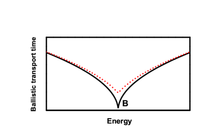
Figure 4: Schematic illustration of the ballistic propagation of tachyonic excitations (electrons with positive group velocity and holes with negative group velocity) through the junction layer between two TIs. At the point of diverging group velocity, the ballistic travel time as a function of electron energy shows a cusp-like singularity (solid line). The finite width of the electron wave packet results in smearing of this singularity (dotted line). Point B corresponds to the singular point in Fig. 1.

In conclusion, we have shown here that for a general set of parameters for the topological insulator Hamiltonian, the surface states at the junction between two TIs have at least one unique tachyonic branch, which describes the propagation of Direc fermion excitations with superluminal group velocity. Although the excitations propagating with superluminal velocity are known (theoretically) to exist in optical systems, we show here that such excitations can actually be realized in purely electronic systems. In these systems, the tachyonic excitations are well localized at the junction between the TIs and are susceptible to direct experimental observation. It would indeed be a remarkable feat for condensed matter and the materials sciences if the first ever signature of elusive tachyons is actually detected experimentally in a topological insulator junction.

The work has been supported by the Canada Research Chairs Program of the Government of Canada.

References

- (1) Electronic address: tapash@physics.umanitoba.ca
- (2) M.Z. Hasan and C.L. Kane, Rev. Mod. Phys. 82, 3045 (2010); X.-L. Qi and S.-C. Zhang, ibid. 83, 1057 (2011).
- (3) D.S.L. Abergel, V. Apalkov, J. Berashevich, K. Ziegler, and T. Chakraborty, Adv. Phys. 59, 261 (2010).
- (4) D. Hsieh, Y. Xia, D. Qian, L. Wray, J. H. Dil, F. Meier, J. Osterwalder, L. Patthey, J.G. Checkelsky, N.P. Ong, A.V. Fedorov, H. Lin, A. Bansil, D. Grauer, Y. S. Hor, R. J. Cava, M.Z. Hasan, Nature 460, 1101 (2009).
- (5) P. Roushan, J. Seo, C.V. Parker, Y.S. Hor, D. Hsieh, D. Qian, A. Richardella, M.Z. Hasan, R.J. Cava, A. Yazdani, Nature 460, 1106 (2009).
- (6) A. Sommerfeld, Nachr. Ges. Wiss. Göttingen, pp. 201-235, February 25, 1905.
- (7) O.M.P. Bilaniuk, V.K. Deshpande, and E.C.G. Sudarshan, Am. J. Phys. 30, 718 (1962); G. Feinberg, Phys. Rev. 159, 1089 (1967); E. Recami, J. Phys. Conf. Ser. 196, 012020 (2009); O.M. Bilaniuk, ibid. 196, 012021 (2009).
- (8) A. Chodos, A.I. Hauser, and V.A. Kostelecky, Phys. Lett. B 150, 431 (1985).
- (9) R. Ehrlich, Am. J. Phys. 71, 1109 (2003).
- (10) E. Recami, Foundation of Physics 31, 1119 (2001).
- (11) C.-X. Liu, X.-L. Qi, H.J. Zhang, X. Dai, Z. Fang, and S.-C. Zhang, Phys. Rev. B 82, 045122 (2010).
- (12) H. Zhang, C.-X. Liu, X.-L. Qi, Xi Dai, Z. Fang, and S.-C. Zhang, Nat. Phys. 5, 438 (2009).
- (13) W.-Y. Shan, H.-Z. Lu, S.-Q. Shen, New J. Phys. 12 043048 (2010).
- (14) B. Zhou, H.Z. Lu, R.L. Chu, S.Q. Shen, and Q. Niu, Phys. Rev. Lett. 101 246807 (2008).
- (15) R. Takahashi, S. Murakami, Phys. Rev. Lett. 107, 166805 (2011).
- (16) R.Y Chiao, A.E. Kozhekin, G. Kurizki, Phys. Rev. Lett. 77, 1254 (1996).
- (17) P.Y. Chen, C.G. Poulton, A.A. Asatryan, M.J. Steel, L.C. Botten, C. Martijn de Sterke, R.C. McPhedran, New J. Phys. 13, 053007 (2011).
- (18) P.W. Milonni, J. Phys. B: At. Mol. Opt. Phys. 35, R31 (2002).
- (19) U.D. Jentschura, Arxiv preprint arXiv:1201.6300 (2012).
- (20) E.A. Shaner and S.A. Lyon, Phys. Rev. Lett. 93, 037402 (2004).