Quantile Mechanics 3: Series Representations and Approximation of some Quantile Functions appearing in Finance.

Abstract

It has long been agreed by academics that the inversion method is the method of choice for generating random variates, given the availability of the quantile function. However for several probability distributions arising in practice a satisfactory method of approximating these functions is not available. The main focus of this paper will be to develop Taylor and asymptotic series expansions for the quantile functions belonging to the following probability distributions; Variance Gamma, Generalized Inverse Gaussian, Hyperbolic and $\alpha$-Stable. As a secondary matter, based on these analytic expressions we briefly investigate the problem of approximating the quantile function.

1 Introduction

Analytic expressions for quantile functions, have long been sought after. The importance of these functions comes from their widespread use in applications of statistics, probability theory, finance and econometrics. Therefore much effort has been devoted into their study, in particular since closed form expressions for the quantile function of most distributions are not known, several approximations appear in the literature. These approximations generally fall into one of four categories, series expansions, functional approximations, numerical algorithms or closed form expressions written in terms of a quantile function of another distribution. The focus of this report is on the former two categories.

For a given distribution function $F$ denote by $Q$ the associated quantile function. We restrict our attention to the class of distributions for which $F$ is strictly increasing and absolutely continuous. In this case we have

$$Q\left(u\right):=F^{-1}\left(u\right)$$ (1.1)

where $F^{-1}$ is the compositional inverse of $F$. Suppose the corresponding density function $f\left(x\right)$ is known. Differentiating (1.1) we obtain the first order quantile equation,

$$\frac{dQ\left(u\right)}{du}=\frac{1}{F^{\prime}\left(F^{-1}\left(u\right)\right)}=\frac{1}{f(Q\left(u\right))}.$$ (1.2)

This is an autonomous equation in which the nonlinear terms are introduced through the density function $f$. Many distributions of interest have complicated densities, for example the densities of the generalized hyperbolic distributions are written in terms of higher transcendental functions. Thus the solutions to (1.2) are often difficult to find, and hence this route has been relatively unexplored in the literature. However provided the reciprocal of the density $1/f$ is an analytic function at the initial condition $x_{0}=Q\left(u_{0}\right)$ we may employ some of the oldest methods of numerical integration of initial value problems, namely the method of undetermined coefficients and the method of successive differentiation, used to determine the Taylor series expansions of $Q$. Since the equations in question are non-linear, finding their solutions requires some special series manipulation techniques found in for example [19]. Shaw and Steinbrecher [42] considered power series solutions to a nonlinear second order differential equation focusing on particular distributions belonging to the Pearson family. We will extend their work here by examining some non-Pearson distributions, in particular we will look at the cases where $f$ is the density function of the hyperbolic, variance gamma, generalized inverse Gaussian and $\alpha$-stable distributions.

The central issue in developing algorithms to approximate the quantile function $Q$ is that near the singular points the condition number $\kappa_{Q}\left(u\right)$ defined by,

$$\kappa_{Q}\left(u\right):=\left|\frac{uQ^{\prime}\left(u\right)}{Q\left(u\right)}\right|$$

is large, resulting in an ill conditioned problem (i.e. near the singular points a small change in $u$ will result in large deviations in $Q$). A remedy to this problem is to introduce a new variable $z$ to reduce $\kappa_{Q}$. As an example consider the quantile function of the standard normal distribution $\Phi^{-1}(u):=\sqrt{2}\textrm{erf}^{-1}\left(2u-1\right)$. The associated condition number $\kappa_{\Phi^{-1}}\left(u\right)$ grows without bound as $u\rightarrow 1$. Hence our problem is ill conditioned near the singular point $u=1$, and one should therefore seek a change of variable to reduce $\kappa_{\Phi^{-1}}\left(u\right)$, for example by introducing the variable $z\left(u\right):=-\ln\left(1-u\right)$. One may then consider the equivalent problem of approximating the transformation $A(z):=\Phi^{-1}(1-e^{-z})$. This approach was first taken in [40], albeit from a slightly different perspective. Of course in the normal case the transformed function $A$ can be written down explicitly, since the form of $Q$ was know. For situations in which this is not possible we formulate a first order differential equation, which we will solve in the subsequent sections for $A$.

To motivate the idea suppose the base distribution used in the inversion method to generate random variates is the standard uniform $U(0,1)$. Once a random variate from this distribution has been generated we may generate a random variate $X$ from the target distribution with c.d.f. $F_{T}$ by setting $X=Q_{T}\left(U\right)$, where $Q_{T}$ is the associated quantile function of the target distribution and $U\sim U\left(0,1\right)$. However as noted by Shaw and Brickman in [40] the base distribution need not be restricted to the standard uniform. Suppose we wish to generate random variates from a target distribution with distribution function $F_{T}$ and associated quantile function $Q_{T}$. Assume further that rather than generating uniform random variates we can generate variates from a base distribution with distribution function $F_{B}$ and associated quantile function $Q_{B}$. Now if we could find a function $A$ which associates the $u^{th}$ quantile from the base distribution with the $u^{th}$ quantile from the target distribution,

$$Q_{T}(u)=A\left(Q_{B}\left(u\right)\right),$$ (1.3)

we could generate random variates from the target distribution simply by setting $X=A\left(Q_{B}\left(U\right)\right).$ Note however the function argument $Z=Q_{B}\left(U\right)$ is itself a random variate from the base distribution. Thus we now have a recipe to generate random variates from a specified target distribution given random variates from a non-uniform base distribution.

There is no restriction on the choice of base distribution, however for the purpose of approximating $Q_{T}$ a wise choice of the variable $z:=Q_{B}\left(u\right)$ would be one that reduces the condition number, $\kappa_{A}\left(z\left(u\right)\right)<\kappa_{Q}\left(u\right)$. We will now derive an ordinary differential equation describing the function $A$ arising from the change of variable. Starting with the first order quantile equation for the target quantile function $Q_{T}$,

$$\frac{dQ_{T}\left(u\right)}{du}=\frac{1}{f_{T}(Q_{T}\left(u\right))},$$ (1.4)

we make a change of variable $z=Q_{B}\left(u\right)$. A simple application of the chain rule for differentiation to (1.3) and using the fact that $Q_{B}$ also satisfies the first order quantile equation gives,

$$\frac{dQ_{T}\left(u\right)}{du}=\frac{dA}{dz}\frac{dz}{du}=\frac{dA}{dz}\frac{dQ_{B}}{du}=\frac{dA}{dz}\frac{1}{f_{B}(Q_{B}\left(u\right))}=\frac{dA}{dz}\frac{1}{f_{B}(z)}.$$

Substituting this identity into (1.4) we obtain a first order nonlinear differential equation,

$$\frac{dA}{dz}=\frac{f_{B}\left(z\right)}{f_{T}(A\left(z\right))},$$ (1.5)

which we call the first order recycling equation. A second order version of this equation was treated in [40].

Note that the idea of expressing target quantiles in terms of base quantiles is not a new one, indeed this is the idea behind the generalized Cornish Fisher expansion, which originally introduced in [11] and [17] was generalized by Hill and Davis in [23]. The Cornish Fisher expansion has many drawbacks however, we refer the interested reader to [24]. Another interesting idea along these lines was introduces by Takemura [44]. Here the the Fourier series expansion of the target quantile $Q_{T}$ is developed with respect to an orthonormal basis of the form $\left\{\psi_{i}\circ Q_{B}\right\}_{i=0}^{\infty}$, where $\left\{\psi_{i}\right\}_{i=0}^{\infty}$ is itself an orthonormal basis for a set of square integrable functions, we refer the reader to the original paper for details. Unlike the Cornish Fisher expansion which is asymptotic in nature Takemura’s approach yields a convergent series in the $L^{2}$ norm. Note however the computation of the Fourier coefficients usually requires numerical quadrature and that for approximation purposes the $L^{\infty}$ norm is preferred.

Standard numerical techniques such as root finding and interpolation for approximating the associated quantile functions often fail, particularly in the tail regions of the distribution, see for example [14]. Thus in addition to developing convergent power series solutions to (1.2) and (1.3) we also develop asymptotic expansions of $Q$ at the singular points $u=0$ and $u=1$. In general it is not easy to discover these asymptotic behaviors, some trial and error and intelligent fiddling is required, [5, Ch. 4]. Our approach is to consider $Q$ as being implicitly defined by the equation,

$$F(Q)=u.$$

Asymptotic iteration methods, see for example [8, Ch. 2], may then be used to obtain the leading terms in the expansion. For numerical purposes the resulting expansions are divergent but may be summed by employing an appropriate summation technique such as Shank’s $e_{k}$ or Levin’s $u$ transforms. The reader is warned that the approach taken throughout the paper is an applied one, the reader will certainly notice a lack of rigor at certain points, in particular in deriving these asymptotic expansions we will execute some “sleazy” maneuvers.

In this report we will focus on the variance gamma, generalized inverse Gaussian, hyperbolic, normal inverse Gaussian and $\alpha$-stable distributions. For each of these distributions we will find power series expansions of $Q$ and $A$ as well as the asymptotic behavior of $Q$ near its singularities. Despite the unsightly appearance of the formulae given in the present paper for the coefficients appearing in these expansions, they are simple to program if not tedious. It is difficult to study analytically the convergence properties of these series, hence we will proceed in an empirical manner. In the last section of this report we experiment with various numerical algorithms to approximate $Q$, observing that a scheme based on Chebyshev-Padé approximants and optimally truncated asymptotic expansions seems most useful.

2 Hyperbolic Distribution

Amongst others it was observed by [16] and [6] the hyperbolic distribution is superior to the normal distribution in modeling log returns of share prices. Numerical inversion of the hyperbolic distribution function was considered in [28]. There numerical methods were considered to solve (1.2) and only the leading order behavior of the left and right tails was given. Here we will provide an analytic solution to (1.2) and the full asymptotic behavior of the tails. The density of the of the hyperbolic distribution $\textrm{Hyp}\left(\alpha,\beta,\delta,\mu\right)$ is given by,

$$f\left(x;\alpha,\beta,\delta,\mu\right)=\frac{\gamma}{2\alpha\delta K_{1}\left(\delta\gamma\right)}e^{-\alpha\sqrt{\delta^{2}+(x-\mu){}^{2}}+\beta(x-\mu)},$$ (2.1)

where $\alpha>0$, $\left|\beta\right|<\alpha$, $\delta>0$ and $\mu\in\mathbb{R}$ are shape, skewness, scale and location parameters respectively and for notational convenience we have set $\gamma=\sqrt{\alpha^{2}-\beta^{2}}$. By defining $\alpha_{1}:=\delta\alpha$ and $\beta_{1}:=\delta\beta$, we obtain an alternative parametrization in which $\alpha_{1}$ and $\beta_{1}$ are now location and scale invariant parameters. Hence without loss of generality we may set $\mu=0$ and $\delta=1$, since $Q\left(u;\alpha_{1},\beta_{1},\mu,\delta\right)=\mu+\delta Q\left(u;\alpha_{1},\beta_{1},0,1\right)$. The first order quantile equation (1.2) then reads,

$$\frac{dQ}{du}=N_{0}e^{\alpha_{1}\sqrt{1+Q^{2}}-\beta_{1}Q}$$ (2.2)

where $N_{0}=2\alpha_{1}\text{K}_{1}\left(\gamma_{1}\right)/\gamma_{1}$ and $\gamma_{1}=\sqrt{\alpha_{1}^{2}-\beta_{1}^{2}}$. To form an initial value problem (IVP) let $u_{0}\in\left(0,1\right)$ and impose the initial condition $Q\left(u_{0}\right)=x_{0}$. For all practical purposes $x_{0}$ is usually determined by solving the equation $F\left(x_{0}\right)-u_{0}=0$ using a root finding procedure. By applying the method of undetermined coefficients we find $Q$ admits the Taylor series expansion,

$$Q\left(u\right)=\sum_{n=0}^{\infty}q_{n}(u-u_{0})^{n},$$

where the coefficients $q_{n}$ are defined recursively as follows,

$$q_{n}\text{=}\begin{cases}x_{\text{0}},&n=0\\ \frac{N_{0}}{n}b_{n-1},&n\geq 1\end{cases},$$

$$b_{n}=\begin{cases}e^{\alpha_{1}\sqrt{1+x_{0}^{2}}-\beta_{1}x_{0}},&n=0\\ \frac{1}{n}\sum_{k=1}^{n}k(\alpha_{1}a_{k}-\beta_{1}q_{k})b_{n-k},&n\geq 1\end{cases},$$

and,

$$a_{n}=\begin{cases}\sqrt{1+x_{0}^{2}}&n=0\\ \frac{1}{na_{0}}\left(nq_{n}q_{0}+\sum_{k=0}^{n-2}(k+1)(q_{k+1}q_{n-k-1}-a_{k+1}a_{n-k-1})\right)&n\geq 1\end{cases}.$$

To develop the asymptotic behavior at the singular points $u=0$ and $u=1$ note that the hyperbolic distribution function $F$ satisfies the relationship,

$$F\left(x;\alpha_{1},\beta_{1},1,0\right)=1-F\left(-x;\alpha_{1},-\beta_{1},1,0\right),$$

which implies,

$$Q\left(u;\alpha_{1},\beta_{1},1,0\right)=-Q\left(1-u;\alpha_{1},-\beta_{1},1,0\right).$$

Hence without loss of generality we need only look for an asymptotic expansion of $Q$ as $u\rightarrow 1$. Now under the assumption $1\ll Q$ as $u\rightarrow 1$, we obtain from (2.2),

$$\frac{dQ}{du}\sim N_{0}e^{\left(\alpha_{1}-\beta_{1}\right)Q},\quad\textrm{as}\;u\rightarrow 1.$$

Solving this asymptotic relationship along with the condition $Q\left(1\right)=\infty$ yields the leading order behavior of $Q$,

$$Q\left(u\right)\sim-\frac{\ln\left(N_{0}\left(\alpha_{1}-\beta_{1}\right)\left(1-u\right)\right)}{\left(\alpha_{1}-\beta_{1}\right)},\quad\textrm{as}\;u\rightarrow 1.$$

From which we note that $Q$ has a logarithmic singularity at $u=1$. To develop further terms in the expansion, write $x:=Q\left(u\right)$ from which it follows $u=F(x)$ and note that $Q$ is implicitly defined by the equation,

$$1-F(x)=\int_{x}^{\infty}f(t)\,dt$$

Rearranging and introducing the variable $v$ we obtain,

$$v\text{:=}(1-u)N_{0}=\int_{x}^{\infty}e^{-\alpha_{1}\sqrt{1+t^{2}}+\beta_{1}t}\,dt.$$

The idea is to expand the integrand appearing in the right hand side and integrate term-wise, this process can be carried out symbolically, giving the first few terms in the expansion,

$$v\sim e^{-x(\alpha_{1}-\beta_{1})}\left(\frac{1}{\alpha_{1}-\beta_{1}}-\frac{\alpha_{1}}{2(\alpha_{1}-\beta_{1})x}+\frac{\alpha_{1}\left(4+\alpha_{1}(\alpha_{1}-\beta_{1})\delta^{2}\right)}{8(\alpha_{1}-\beta_{1})^{2}x^{2}}+O\left(\frac{1}{x^{3}}\right)\right).$$

Taking logs and inverting the resulting series allows us to write down the first few terms in the asymptotic expansion of $x$,

$$x\sim y+\frac{\alpha_{1}}{2\left(\alpha_{1}-\beta_{1}\right)y}+\frac{\alpha_{1}}{2\left(\alpha_{1}-\beta_{1}\right)^{2}y^{2}}+O\left(\frac{1}{y^{3}}\right)$$

from which we can conjecture the form the asymptotic expansion of $Q$ as,

$$Q(u)\sim y+\sum_{n=1}^{\infty}\frac{q_{n}}{y^{n}},\quad\textrm{as}\;u\rightarrow 1,$$ (2.3)

where,

$$y=-\frac{\ln\left(N_{0}\left(\alpha_{1}-\beta_{1}\right)\left(1-u\right)\right)}{\left(\alpha_{1}-\beta_{1}\right)}.$$

Substituting (2.3) into the first order quantile equation (2.2) allows us to derive a recurrence relationship for the coefficients $q_{n}$,

$$q_{n}\text{=}\begin{cases}0&n=0\\ -\frac{\alpha_{1}}{2(\alpha_{1}-\beta_{1})}&n=1\\ -\frac{1}{(\alpha_{1}-\beta_{1})}\left((n-1)q_{n-1}+\frac{1}{n}\sum_{k=1}^{n-1}kb_{k}c_{n-k}+\alpha_{1}d_{n}\right)&n\geq 2\end{cases},$$

where,

$$a_{n}\text{=}\begin{cases}0&n=0\\ \frac{1}{2}+q_{1}&n=1\\ q_{n}+d_{n}&n\geq 2\end{cases},$$

$$b_{n}=\alpha_{1}a_{n}-\beta_{1}q_{n},$$

$$c_{n}\text{=}\begin{cases}1&n=0\\ \frac{1}{n}\sum_{k=1}^{n}kb_{k}c_{n-k}&n\geq 1\end{cases},$$

and,

$$d_{n}=\frac{1}{n-1}\sum_{k=0}^{n-2}(k+1)(q_{k+1}q_{n-k-2}-a_{k+1}a_{n-k-2}).$$

Note that (2.3) is a divergent series, however of the summation methods we tested we found Levin’s $u$ transform and Padé approximants particular useful for summing (2.3). In both cases analytic continuation was observed. Later we will briefly look at algorithms for constructing rational approximants of $Q$ valid on the domain $\left[10^{-10},1-10^{-10}\right]$, but if necessary one may utilize (2.3) to obtain approximations on a wider region.

As mentioned in the introduction the problem of approximating the quantile function near its singular points is an ill conditioned one. To this end it will be useful to introduce a change of variable which reduces the condition number $\kappa_{Q}$. Motivated by the asymptotic behavior of $Q$ near its singular points, in particular its leading order behavior we introduce the base distribution defined by the density,

$$f_{B}\left(x\right):=\begin{cases}p_{-}\left(\alpha_{1}+\beta_{1}\right)e^{\left(\alpha_{1}+\beta_{1}\right)x},&x\leq x_{m}\\ p_{+}\left(\alpha_{1}-\beta_{1}\right)e^{-\left(\alpha_{1}-\beta_{1}\right)x},&x>x_{m}\end{cases}.$$

Here $x_{m}:=\beta_{1}/\gamma_{1}$ is the mode of the hyperbolic distribution, $p_{-}:=e^{-(\text{$\alpha$1}+\text{$\beta$1})x_{m}}p_{m}$, $p_{+}:=e^{(\text{$\alpha$1}-\text{$\beta$1})x_{m}}\left(1-p_{m}\right)$ and $p_{m}=F_{T}\left(x_{m}\right)$. The associated distribution and quantile functions can be written down as,

$$F_{B}\left(x\right):=\begin{cases}p_{-}e^{\left(\alpha_{1}+\beta_{1}\right)x},&x\leq x_{m}\\ 1-p_{+}e^{-\left(\alpha_{1}-\beta_{1}\right)x},&x>x_{m}\end{cases},$$

and,

$$Q_{B}\left(u\right)=\begin{cases}\frac{1}{\alpha_{1}+\beta_{1}}\ln\left(\frac{u}{p_{-}}\right),&u\leq p_{m}\\ -\frac{1}{\alpha_{1}-\beta_{1}}\ln\left(\frac{1-u}{p_{+}}\right),&u>p_{m}\end{cases},$$

respectively. Substituting this choice of $f_{B}$ into the recycling equation (1.5) results in a left and right problem,

$$\frac{dA}{dz}=p_{-}(\alpha_{1}+\beta_{1})Ce^{\alpha_{1}\sqrt{1+A^{2}}-\beta_{1}A+\left(\alpha_{1}+\beta_{1}\right)z},\quad z\leq x_{m},$$

and

$$\frac{dA}{dz}=p_{+}(\alpha_{1}-\beta_{1})Ce^{\alpha_{1}\sqrt{1+A^{2}}-\beta_{1}A-\left(\alpha_{1}-\beta_{1}\right)z},\quad z>x_{m},$$

respectively, along with the suitably imposed initial conditions. For the left problem, we choose $u_{0}\in\left(0,p_{m}\right]$ and impose the initial condition $x_{0}=A\left(z_{0}\right)=Q_{T}\left(u_{0}\right)$, where $z_{0}:=Q_{B}\left(u_{0}\right)$. Similarly for the right problem choose $u_{0}\in\left[p_{-},1\right)$. Again through the method of undetermined coefficients we obtain the Taylor series expansion of $A$,

$$A\left(z\right)=\sum_{n=0}^{\infty}a_{n}(z-z_{0})^{n},$$

where the coefficients are defined recursively by,

$$a_{n}=\begin{cases}x_{0}&n=0\\ \frac{C}{n}\theta\left(\alpha_{1}+\beta_{1}\right)d_{n-1}&n\geq 1\end{cases},$$

$$b_{n}=\begin{cases}\sqrt{1+x_{0}^{2}}&n=0\\ \frac{1}{nb_{0}}\left(na_{n}a_{0}+\sum_{k=0}^{n-2}(k+1)\left(a_{k+1}a_{n-k-1}-b_{k+1}b_{n-k-1}\right)\right)&n\geq 1\end{cases},$$

$$c_{n}=\begin{cases}\alpha_{1}\left(b_{1}+\phi\right)+\beta_{1}\left(1-a_{1}\right)&n=1\\ \alpha_{1}b_{n}-\beta_{1}a_{n}&n\neq 1\end{cases},$$

and,

$$d_{n}=\begin{cases}e^{\alpha_{1}\sqrt{1+x_{0}^{2}}-\beta_{1}x_{0}+\rho z_{0}}&n=0\\ \frac{1}{n}\sum_{k=1}^{n}kc_{k}d_{n-k}&n\geq 1\end{cases}.$$

For the solution to the left and right problem make the following replacements,

Table 1: Coefficient Parameters

	Left	Right
$\theta$	$p_{-}$	$p_{+}$
$\phi$	$+1$	$-1$
$\rho$	$\left(\alpha_{1}+\beta_{1}\right)$	$-\left(\alpha_{1}-\beta_{1}\right)$

3 Variance Gamma

The variance gamma distribution was introduced in the finance literature by Madan and Seneta in [30]. To our knowledge there has been very little written on the approximation of the variance gamma quantile. The density is given by,

$$f_{\textrm{VG}}\left(x;\lambda,\alpha,\beta,\mu\right)=\frac{\gamma^{2\lambda}}{\left(2\alpha\right)^{\lambda-1/2}\sqrt{\pi}\Gamma\left(\lambda\right)}\left|x-\mu\right|^{\lambda-\frac{1}{2}}\textrm{K}_{\lambda-\frac{1}{2}}\left(\alpha\left|x-\mu\right|\right)e^{\beta\left(x-\mu\right)},$$ (3.1)

where $\lambda>0$, $\alpha>0$, $\left|\beta\right|<\alpha$, $\gamma=\sqrt{\alpha-\beta}$ and $\mu\in\mathbb{R}$. Setting the location parameter $\mu$ to zero and substituting the density (3.1) into the quantile equation (1.2) gives,

$$\frac{dQ}{du}=g(Q(u))$$ (3.2)

where the function $g$ is defined as,

$$g\left(y\right):=N_{0}\frac{e^{-\beta y}|y|^{\frac{1}{2}-\lambda}}{\textrm{K}_{\lambda-\frac{1}{2}}(\alpha|y|)}.$$

and $N_{0}=\left(2\alpha\right)^{\lambda-1/2}\sqrt{\pi}\Gamma\left(\lambda\right)/\gamma^{2\lambda}$. Our strategy to solve (3.2) will be to apply the method of successive differentiation to obtain the Taylor series representation of $Q$,

$$Q_{\textrm{VG}}\left(u\right)=\sum_{n=0}^{\infty}q_{n}(u-u_{0})^{n}$$ (3.3)

where $q_{0}$ is determined by the imposed initial condition, and the remaining coefficients are given by,

$$q_{n}=\left.\frac{d^{n-1}}{du^{n-1}}\right|_{u=u_{0}}g\left(Q\left(u\right)\right),\quad n\geq 1$$

Thus the problem reduces to finding the higher order derivatives of the composition $g\circ Q$, which can be obtained recursively through by applying Faà di Bruno’s formula as follows. Note first that $g$ can be written as the product of three functions $a\left(y\right):=e^{-\beta y}$, $b\left(y\right):=|y|^{\frac{1}{2}-\lambda}$ and $c\left(y\right):=\left[K_{\lambda-\frac{1}{2}}(\alpha|y|)\right]^{-1}$. Thus an application of the general Leibniz rule yields,

$$g^{\left(n\right)}\left(y\right)=N_{0}\sum_{k=0}^{n}\sum_{j=0}^{k}\binom{n}{k}\binom{k}{j}a^{\left(n-k\right)}\left(y\right)b^{\left(j\right)}\left(y\right)c^{\left(k-j\right)}\left(y\right).$$ (3.4)

The higher order derivatives of the functions $a$ and $b$ appearing in (3.4) are given by,

$$a^{(n)}\left(y\right)=\left(-\beta\right)^{n}e^{-\beta y},$$

$$b^{(n)}\left(y\right)=y^{\frac{1}{2}-n-\lambda}\prod_{i=0}^{n-1}\left(\frac{1}{2}-\lambda-i\right)\times\begin{cases}+1&y>0\\ -1&y<0\end{cases}.$$

To find the $n^{th}$ derivative of $c$ note that $c$ can be written as the composition $c\left(y\right)=c_{1}\circ c_{2}\left(y\right)$, where $c_{1}\left(y\right):=1/y$ and $c_{2}\left(y\right):=K_{\lambda-\frac{1}{2}}(\alpha|y|)$. Hence we may obtain $c^{\left(n\right)}\left(y\right)$ through an application of Faà di Bruno’s formula,

$$c^{\left(n\right)}\left(y\right)=\sum\frac{n!}{m_{1}!m_{2}!\cdots m_{n}!}c_{1}^{\left(m_{1}+\cdots+m_{n}\right)}\left(c_{2}\left(y\right)\right)\prod_{j=0}^{n}\left(\frac{c_{2}^{\left(j\right)}\left(y\right)}{j!}\right)^{m_{j}},$$

where the summation is taken over all solutions $\left(m_{1},m_{2},\ldots,m_{n}\right)\in\mathbb{Z}_{\geq 0}^{n}$ to the Diophantine equation,

$$m_{1}+2m_{2}+3m_{3}\cdots+nm_{n}=n.$$ (3.5)

The formulae for the higher order derivatives of $c_{1}$ and $c_{2}$ are given by,

$$c_{1}^{(n)}\left(y\right)=\left(-1\right)^{n}n!y^{-(n+1)},$$

and

$$c_{2}^{\left(n\right)}\left(y\right)=\left(-\frac{\alpha}{2}\right)^{n}\sum_{k=0}^{n}\binom{n}{k}\times\begin{cases}\textrm{K}_{\lambda-\frac{1}{2}-(2k-n)}(\alpha y),&y>0\\ \left(-1\right)^{n}\textrm{K}_{\lambda-\frac{1}{2}-(2k-n)}(-\alpha y)&y<0\end{cases}.$$

Where we have used the identity [33, eq. 10.29.5],

$$\textrm{K}_{v}^{\left(n\right)}\left(z\right)=\left(-\frac{1}{2}\right)^{n}\sum_{k=0}^{n}\binom{n}{k}\textrm{K}_{v-\left(2k-n\right)}\left(z\right),$$ (3.6)

which can easily be proved by induction. Formula (3.6) shows that, to find the higher order derivatives with respect to $z$ of the modified Bessel function of the second kind $\textrm{K}_{v}^{\left(n\right)}\left(z\right)$ we need only a routine to compute $\textrm{K}_{v}\left(z\right)$. Now given the scheme (3.4) to compute $g^{\left(n\right)}\left(x\right)$ and the coefficient $q_{0}$ defined by the initial condition we may then compute $q_{n}$ for $n\geq 1$ recursively, by another application of Faà di Bruno’s formula. It is important to note that to generate the coefficients $q_{n}$ appearing in (3.3) does not require the use of any symbolic computation.

Next we will focus on deriving an asymptotic expansion for $Q\left(u\right)$. Similar to the hyperbolic quantile the following equality holds,

$$Q\left(u;\lambda,\alpha,\beta,0\right)=-Q\left(1-u;\lambda,\alpha,-\beta,0\right),$$

so again without loss of generality we need only seek an asymptotic expansion of $Q$ as $u\rightarrow 1$. Our strategy here will be to,

1. derive an asymptotic expansion for the density $f$ as $x\rightarrow\infty$,

2. integrate term-wise to obtain an asymptotic expansion for the distribution function $F$ as $x\rightarrow\infty$,

3. and finally invert this expansion to obtain an asymptotic expansion for the quantile function $Q$ as $u\rightarrow 1$.

For the first step we will make use of the asymptotic relationship [33, §10.40],

$$\textrm{K}_{v}\left(z\right)\sim\left(\frac{\pi}{2z}\right)^{\frac{1}{2}}e^{-z}\sum_{k=0}^{\infty}\frac{a_{k}\left(v\right)}{z^{k}}\quad\textrm{as}\;z\rightarrow\infty,$$

where,

$$a_{k}\left(v\right):=\frac{1}{k!8^{k}}\prod_{j=1}^{k}\left(4v^{2}-(2j-1)^{2}\right).$$

From which it follows

$$f\left(x\right)\sim\frac{\gamma^{2\lambda}}{\left(2\alpha\right)^{\lambda}\Gamma\left(\lambda\right)}e^{-\left(\alpha-\beta\right)x}x^{\lambda-1}\sum_{k=0}^{\infty}\frac{a_{k}\left(\lambda-\frac{1}{2}\right)}{\alpha^{k}}x^{-k}\quad\textrm{as}\;x\rightarrow\infty.$$

Working under the assumption that term-wise integration is a legal operation we obtain an asymptotic expansion for the distribution function,

$$1-F\left(x\right) \sim \frac{\gamma^{2\lambda}}{2^{\lambda}\Gamma\left(\lambda\right)}\sum_{k=0}^{\infty}\alpha^{-\lambda-k}a_{k}\left(\lambda-2^{-1}\right)\int_{x}^{\infty}e^{-\left(\alpha-\beta\right)x}t^{\lambda-k-1}dt$$ (3.7)

$$= \frac{\gamma^{2\lambda}}{2^{\lambda}\Gamma\left(\lambda\right)}\sum_{k=0}^{\infty}\alpha^{-\lambda-k}a_{k}\left(\lambda-2^{-1}\right)\Gamma\left(\lambda-k,x\left(\alpha-\beta\right)\right),$$

where $\Gamma\left(a,z\right)$ is the upper incomplete gamma function, which for large $z$ satisfies the asymptotic relationship [33, §8.11],

$$\Gamma\left(a,z\right)\sim z^{a-1}e^{-z}\sum_{j=0}^{\infty}\frac{\Gamma\left(a\right)}{\Gamma\left(a-j\right)}z^{-j}.$$ (3.8)

Substituting into (3.7) and assuming the terms of the series may be rearranged we obtain,

$$1-F\left(x\right)\sim\frac{\left(2\alpha\right)^{-\lambda}\gamma^{2\lambda}}{\Gamma(\lambda)}x^{\lambda-1}e^{-x(\alpha-\beta)}\sum_{k=0}^{\infty}b_{k}x^{-k}\quad\textrm{as}\;x\rightarrow\infty,$$ (3.9)

where,

$$b_{k}=\sum_{j=0}^{k}(\alpha-\beta)^{-(j+1)}\alpha^{-(k-j)}\left(\prod_{i=0}^{k-1}(\lambda-k+i)\right)a_{k-j}\left(\lambda-\frac{1}{2}\right).$$

The expression (3.9) describes the asymptotic behavior of the variance gamma distribution function as $x\rightarrow\infty$. Let $u=F\left(x\right)$ in (3.9), our goal then is to invert this relationship to obtain an asymptotic expansion of the quantile function $Q\left(u\right)$ as $u\rightarrow 1$. Introducing the variable,

$$v\text{:=}\frac{(2\alpha)^{\lambda}\sqrt{\pi}\Gamma(\lambda)}{\gamma^{2\lambda}}(1-u),$$

and rearranging (3.9) we obtain,

$$v\sim x^{\lambda-1}e^{-x(\alpha-\beta)}D\left(\frac{1}{x}\right)\quad\textrm{as}\;x\rightarrow\infty.$$ (3.10)

where $D$ is the formal power series defined by $D\left(z\right)=\sum_{k=0}^{\infty}b_{k}z^{k}$. Taking logs and introducing the variable $y:=-\ln v/\left(\alpha-\beta\right)$, we may write (3.10) as,

$$x\sim y+\frac{\lambda-1}{\alpha-\beta}\log x+\frac{1}{\alpha-\beta}\log D\left(\frac{1}{x}\right)$$ (3.11)

We wish to write $x$ in terms $y$; this task might at first may appear difficult to achieve, but as it happens we are in luck, similar expressions occur frequently in analytic number theory, and some useful methods have been developed to invert these kinds of relationships. A drawback of these methods is that they require symbolic computation. The most basic method known to us, one can apply to invert (3.11) is the method of asymptotic iteration [8]. This method however is extremely slow. A much more efficient approach is to use the method of Salvy[13]. There it was noted that the form of the asymptotic inverse is given by,

$$x=Q\left(u\right)\sim y+\sum_{n=0}^{\infty}\frac{P_{n}\left(\textrm{ln}y\right)}{y^{n}},$$

where $P_{0}\left(\xi\right)$ is a polynomial of degree 1 and $P_{n}\left(\xi\right)$ are polynomials of degree $n$ for $n\geq 1$. Following a similar analysis of that in [13] it can by shown that $P_{n}$ may be determined up to some unknown constant terms $c_{0},\ldots,c_{n}$ by the recurrence relationship,

$$P_{n}\left(\xi\right)=\begin{cases}\frac{(\lambda-1)}{(\alpha-\beta)}\xi+c_{0}&n=0\\ \frac{(\lambda-1)}{(\alpha-\beta)}(P_{n-1}\left(\xi\right)-P_{n-1}\left(0\right))-\frac{(\lambda-1)}{(\alpha-\beta)}(n-1)\int_{0}^{\xi}P_{n-1}\left(t\right)\,dt+c_{n}&n\geq 0\end{cases}.$$ (3.12)

The unknown terms $c_{0},\ldots,c_{n}$ may be computed through the following iteration scheme,

• starting with $u_{0}\left(t\right)=\log\left(b_{0}\right)$, compute,

  $$u_{k}\left(t\right)=\frac{(\lambda-1)}{(\alpha-\beta)}\log\left(1+tu_{k-1}\left(t\right)\right)+\frac{1}{\alpha-\beta}\log D\left(\frac{t}{1+tu_{k-1}\left(t\right)}\right),\quad k=1,\ldots,n+1,$$

• extract the constants,

  $$c_{k}=\left[t^{k}\right]u_{n+1}\left(t\right),\quad k=0,\ldots,n$$

  where $\left[t^{k}\right]u_{n+1}\left(t\right)$ is used to denote the coefficient of the $t^{k}$ term in $u_{n+1}\left(t\right)$.

An implementation of this scheme in Mathematica code has been included in appendix (TODO: Include code). Through this process the first few terms of the asymptotic expansion of $Q$ may be generated as follows,

$$Q\left(u\right) \sim y+\frac{(\lambda-1)\log y-\log\left(\alpha-\beta\right)}{\alpha-\beta}$$

$$\quad+\frac{(\lambda-1)\left(2\alpha+\alpha\lambda-\beta\lambda+2\alpha(\lambda-1)\log y-2\alpha\log\left(\alpha-\beta\right)\right)}{2y\alpha(\alpha-\beta)^{2}}+\cdots,\quad\textrm{as}\;u\rightarrow 1.$$

Next we focus on introducing a change of variable to reduce the condition number $\kappa_{Q}$ near the tails and finding the Taylor series representation of the corresponding function $A$. As in the hyperbolic case motivated by the asymptotic behavior of the quantile function near its singularities, in particular by its leading order behavior we introduce the base distribution defined by the density,

$$f_{B}\left(x\right):=\begin{cases}p_{-}\left(\alpha+\beta\right)e^{\left(\alpha+\beta\right)x}&x\leq 0\\ p_{+}\left(\alpha-\beta\right)e^{-\left(\alpha-\beta\right)x}&x>0\end{cases},$$

where $p_{-}=F\left(0\right)$ and $p_{+}=1-p_{-}$. The associated distribution and quantile functions can be written down as,

$$F_{B}\left(x\right):=\begin{cases}p_{-}e^{\left(\alpha_{1}+\beta_{1}\right)x},&x\leq 0\\ 1-p_{+}e^{-\left(\alpha_{1}-\beta_{1}\right)x},&x>0\end{cases},$$

and,

$$Q_{B}\left(u\right)=\begin{cases}\frac{1}{\alpha_{1}+\beta_{1}}\ln\left(\frac{u}{p_{-}}\right),&u\leq p_{-}\\ -\frac{1}{\alpha_{1}-\beta_{1}}\ln\left(\frac{1-u}{p_{+}}\right),&u>p_{-}\end{cases},$$

respectively. Substituting this choice of $f_{B}$ into the recycling equation (1.5) results in a left and right problem,

$$\frac{dA}{dz}=g_{L}(z),\quad z\leq Q_{B}\left(p_{-}\right),$$

and

$$\frac{dA}{dz}=g_{R}(z),\quad z>Q_{B}\left(p_{-}\right),$$

respectively, along with the suitably imposed initial conditions. For the left problem, we choose $u_{0}\in\left(0,p_{-}\right]$ and impose the initial condition $x_{0}=A\left(z_{0}\right)=Q_{T}\left(u_{0}\right)$, where $z_{0}:=Q_{B}\left(u_{0}\right)$. Similarly for the right problem choose $u_{0}\in\left[p_{-},1\right)$. The functions $g_{L}$ and $g_{R}$ appearing on right hand side of these differential equations are defined as,

$$g_{\textrm{L}}\left(z\right):=p_{-}(\alpha+\beta)e^{(\alpha+\beta)z}g\left(A\left(z\right)\right),$$

and,

$$g_{\textrm{R}}\left(z\right):=p_{+}(\alpha-\beta)e^{-(\alpha-\beta)z}g\left(A\left(z\right)\right).$$

Suppose that the series solution of either problem is given by,

$$A\left(z\right)=\sum_{n=0}^{\infty}a_{n}(z-z_{0})^{n}.$$

Here the first coefficient $a_{0}$ is determined by the initial condition imposed at $z_{0}$ and the remaining coefficients are given by,

$$a_{n}=g_{\textrm{L}}^{\left(n-1\right)}\left(z_{0}\right),\quad n\geq 1,$$

for the left problem and,

$$a_{n}=g_{\textrm{R}}^{\left(n-1\right)}\left(z_{0}\right),\quad n\geq 1,$$

for the right problem. Both sets of coefficients may easily be computed from an application of Liebniz’s rule,

$$g_{\textrm{L}}^{\left(n\right)}\left(z\right)=p_{-}e^{(\alpha+\beta)z}\sum_{k=0}^{n}\binom{n}{k}(\alpha+\beta)^{k+1}\left(g\circ A\right)^{\left(n-k\right)}\left(z\right),$$

$$g_{\textrm{R}}^{\left(n\right)}\left(z\right)=p_{+}e^{-(\alpha-\beta)z}\sum_{k=0}^{n}\binom{n}{k}\left(-1\right)^{k}(\alpha-\beta)^{k+1}\left(g\circ A\right)^{\left(n-k\right)}\left(z\right).$$

Starting with $a_{0}$, the higher order derivatives of the composition $g\circ A$ appearing in these formulae, are computed recursively in precisely the same way we computed the higher order derivatives of $g\circ Q$ above.

4 Generalized Inverse Gaussian

The generalized inverse Gaussian (GIG) is a three parameter distribution, special cases of which are the inverse Gaussian, positive hyperbolic and Lévy distributions to name a few. It arises naturally in the context of first passage times of a diffusion process. The probability density function of a GIG random variable is given by,

$$f_{\textrm{GIG}}\left(x;\lambda,\chi,\psi\right)=\frac{\left(\psi/\chi\right)^{\lambda/2}}{2\textrm{K}_{\lambda}\left(\sqrt{\psi\chi}\right)}x^{\lambda-1}e^{-\frac{1}{2}\left(\chi x^{-1}+\psi x\right)},\quad x>0,$$ (4.1)

where $\lambda\in\mathbb{R}$, $\chi>0$, $\psi>0$ and $\textrm{K}_{v}\left(z\right)$ is the modified Bessel function of the third kind with index $v$. The GIG distribution is also used in the construction of an important family of distributions called the generalized hyperbolic distributions; more specifically a normal mean mixture distribution where the mixing distribution is the GIG distribution results in a generalized hyperbolic distribution. Consequently if one can generate GIG random variates then a simple transformation may be applied to generate variates from the generalized hyperbolic distribution [48].

We will use an alternative parametrization to the standard one above, let $\eta=\sqrt{\chi/\psi}$ and $\omega=\sqrt{\chi\psi}$, the density then reads,

$$f_{\textrm{GIG}}\left(x;\lambda,\eta,\omega\right)=\frac{1}{2\eta^{\lambda}\textrm{K}_{\lambda}\left(\omega\right)}x^{\lambda-1}e^{-\frac{\omega}{2}\left(\eta x^{-1}+\frac{1}{\eta}x\right)}.$$ (4.2)

In this new parametrization $\omega$ and $\lambda$ are scale invariant and $\eta$ is a scale parameter, so in the following without loss of generality we may set $\eta=1$. The first order quantile equation (1.2) now reads,

$$\frac{dQ}{du}=2\text{K}_{\lambda}\left(\omega\right)e^{\frac{1}{2}\omega\left(\frac{1}{Q}+Q\right)}Q{}^{1-\lambda}.$$

Let $u_{0}\in\left(0,1\right)$ and impose the initial condition $Q\left(u_{0}\right)=x_{0}$. For the case $\lambda\neq 1$, the GIG quantile $Q$ admits the Taylor series expansion,

$$Q\left(u\right)=\sum_{n=0}^{\infty}q_{n}(u-u_{0})^{n},$$ (4.3)

where the coefficients $q_{n}$ are defined recursively as follows,

$$q_{n}=\begin{cases}x_{0}&n=0\\ \frac{2}{n}K_{\lambda}(\omega)\sum_{i=0}^{n-1}b_{i}c_{n-i-1}&n\geq 1\end{cases},$$

$$a_{n}=\begin{cases}\frac{1}{q_{0}}&n=0\\ -\frac{1}{q_{0}}\sum_{i=1}^{n}q_{i}a_{n-i}&n\geq 1\end{cases},$$

$$b_{n}=\begin{cases}e^{\frac{\omega}{2}\left(a_{0}+q_{0}\right)}&n=0\\ \frac{\omega}{2n}\sum_{i=1}^{n}i\left(a_{i}+q_{i}\right)b_{n-i}&n\geq 1\end{cases},$$

and

$$c_{n}=\begin{cases}q_{0}^{1-\lambda}&n=0\\ \frac{1}{q_{0}}\sum_{i=1}^{n}\left(\frac{(2-\lambda)i}{n}-1\right)q_{i}c_{n-i}&n\geq 1\end{cases}.$$

For the special case $\lambda=1$, the coefficients are somewhat simplified, with $a_{n}$ and $b_{n}$ as above the coefficients appearing in (4.3) become,

$$q_{n}=\begin{cases}x_{0}&n=0\\ \frac{2}{n}K_{1}(\omega)b_{n-1}&n\geq 1\end{cases}.$$

Next we will focus on developing the asymptotic behavior of $Q$ as $u\rightarrow 1$. We proceed in an analogous fashion to the variance gamma case, and find that remarkably the form of asymptotic expansion of $Q_{\textrm{GIG}}$ is very similar to that of $Q_{\textrm{VG}}$ as $u\rightarrow 1$. From the definition of the distribution function we have,

$$1-F\left(x\right)=\frac{1}{2K_{\lambda}(\omega)}\int_{x}^{\infty}t^{\lambda-1}e^{-\frac{1}{2}\left(\frac{1}{t}+t\right)\omega}dt.$$

Expanding the $e^{-\omega/2t}$ term and integrating term-wise we obtain,

$$1-F\left(x\right)\sim\frac{1}{2K_{\lambda}(\omega)}\sum_{k=0}^{\infty}\frac{(-1)^{k}}{k!}\left(\frac{2}{\omega}\right)^{\lambda-2k}\Gamma\left(\lambda-k,\frac{\omega x}{2}\right),\quad\textrm{as}\;x\rightarrow\infty,$$

where $\Gamma\left(a,z\right)$ is the upper incomplete gamma function. As in the variance gamma case substituting (3.8) and rearranging the terms provides us with a more convenient form of the asymptotic expansion for the generalized inverse Gaussian distribution function,

$$1-F\left(x\right)\sim\frac{1}{2K_{\lambda}(\omega)}x^{\lambda-1}e^{-\frac{\omega x}{2}}\sum_{k=0}^{\infty}b_{k}x^{-k},\quad\textrm{as}\;x\rightarrow\infty,$$ (4.4)

where,

$$b_{k}=\sum_{j=0}^{k}\frac{(-1)^{k-j}}{(k-j)!}\left(\frac{\omega}{2}\right)^{k-2j-1}\left(\prod_{i=0}^{j-1}(\lambda-k+i)\right).$$

Now let $u=F\left(x\right)$ and introduce the variable $v=2K_{\lambda}(\omega)(1-u)$, then we can rewrite (4.4) as,

$$v\sim x^{\lambda-1}e^{-\frac{\omega x}{2}}D(\frac{1}{x}),$$ (4.5)

where $D$ is the formal power series defined by $D\left(z\right)=\sum_{k=0}^{\infty}b_{k}z^{k}$. To invert the asymptotic relationship (4.5) we start by taking logs and introducing the variable $y:=-(2/\omega)\ln v$. We may now write (4.5) as,

$$x\sim y+\frac{2(\lambda-1)}{\omega}\log x+\frac{2}{\omega}\log D\left(\frac{1}{x}\right).$$ (4.6)

One may now apply the method of asymptotic iteration [8] to invert (4.6). As mentioned earlier this method however is extremely slow and a much more efficient approach is to use the method of Salvy[13]. Again the form of the asymptotic inverse is given by,

$$x=Q\left(u\right)\sim y+\sum_{n=0}^{\infty}\frac{P_{n}\left(\textrm{ln}y\right)}{y^{n}},$$

where $P_{0}\left(\xi\right)$ is a polynomial of degree 1 and $P_{n}\left(\xi\right)$ are polynomials of degree $n$ for $n\geq 1$ and following a similar analysis of that in [13] it can by shown that $P_{n}$ may be determined up to some unknown constant terms $c_{0},\ldots,c_{n}$ by the recurrence relationship,

$$P_{n}\left(\xi\right)=\begin{cases}\frac{2(\lambda-1)}{\omega}\xi+c_{0}&n=0\\ \frac{2(\lambda-1)}{\omega}(P_{n-1}\left(\xi\right)-P_{n-1}\left(0\right))-\frac{2(\lambda-1)}{\omega}(n-1)\int_{0}^{\xi}P_{n-1}\left(t\right)\,dt+c_{n}&n\geq 0\end{cases}.$$ (4.7)

The unknown terms $c_{0},\ldots,c_{n}$ may be computed through the following iteration scheme,

• starting with $u_{0}\left(t\right)=\log\left(b_{0}\right)$, compute,

  $$u_{k}\left(t\right)=\frac{2(\lambda-1)}{\omega}\log\left(1+tu_{k-1}\left(t\right)\right)+\frac{2}{\omega}\log D\left(\frac{t}{1+tu_{k-1}\left(t\right)}\right),\quad k=1,\ldots,n+1,$$

• extract the constants,

  $$c_{k}=\left[t^{k}\right]u_{n+1}\left(t\right),\quad k=0,\ldots,n$$

  where $\left[t^{k}\right]u_{n+1}\left(t\right)$ is used to denote the coefficient of the $t^{k}$ term in $u_{n+1}\left(t\right)$.

Through this process the first few terms of the asymptotic expansion of $Q$ may be generated as follows,

$$Q\left(u\right) \sim y+\frac{2\left((-1+\lambda)\ln y+\ln\left(\frac{2}{\omega}\right)\right)}{\omega}$$

$$\quad+\frac{4\lambda-\omega^{2}-4+4(-1+\lambda)^{2}\ln y+4(-1+\lambda)\ln\left(\frac{2}{\omega}\right)}{\omega^{2}y}+\cdots,\quad\textrm{as}\;u\rightarrow 1.$$

To observe the asymptotic behavior of $Q\left(u\right)$ as $u\rightarrow 0$, we utilize the following identity,

$$Q\left(u;\lambda,1,\omega\right)=\frac{1}{Q\left(1-u;-\lambda,1,\omega\right)},$$ (4.8)

which can be easily proven as follows; by definition of the density (4.2) we have,

$$f\left(x;\lambda,1,\omega\right)=\frac{1}{x^{2}}f\left(\frac{1}{x};-\lambda,1,\omega\right).$$

Integrating both sides then yields,

$$F\left(x;\lambda,1,\omega\right)=1-F\left(\frac{1}{x};-\lambda,1,\omega\right),$$

from which (4.8) follows.

Next we consider solving the recycling ODE, but first we must choose a base distribution. Again motivated by the asymptotic behavior of $Q$ as $u\rightarrow 0$ and $u\rightarrow 1$, in particular the leading order behaviors we suggest the following base distribution characterized by the density function,

$$f_{B}\left(x\right)=\begin{cases}p_{\textrm{L}}\frac{\omega}{2x^{2}}e^{-\frac{\omega}{2x}},&x\leq x_{m}\\ p_{\textrm{R}}\frac{\omega}{2}e^{-\frac{\omega}{2}x},&x>x_{m}\end{cases}.$$ (4.9)

Here $x_{m}$ serves as a cutoff point between two suitably weighted density functions, in particular $x_{m}$ is the mode of the GIG distribution defined by,

$$x_{m}=\frac{\lambda-1+\sqrt{(\lambda-1)^{2}+\omega^{2}}}{\omega}.$$

Note that the density function $f_{L}\left(x\right):=(\omega/2x^{2})e^{-\omega/2x}$ belongs to the scaled inverse $\chi^{2}$ distribution with $2$ degrees of freedom and scale parameter $\omega/2$, and that the density function $f_{R}\left(x\right):=(\omega/2)e^{-\omega x/2}$ is the density of an exponential distribution with rate parameter $\omega/2$. The normalizing constants $p_{\textrm{L}}$ and $p_{\textrm{R}}$ are defined by,

$$p_{\textrm{L}}=e^{\frac{\omega}{2x_{m}}}p_{m},$$

and,

$$p_{\textrm{R}}=e^{\frac{\omega}{2}x_{m}}\left(1-p_{m}\right),$$

where $p_{m}=F_{\textrm{GIG}}\left(x_{m}\right).$ The associated distribution and quantile functions can be written down as,

$$F_{B}\left(x\right)=\begin{cases}p_{\textrm{L}}e^{-\frac{\omega}{2x}},&x\leq x_{m}\\ 1-\left(1-p_{\textrm{R}}\right)e^{-\frac{\omega}{2}\left(x-x_{m}\right)},&x>x_{m}\end{cases},$$

and,

$$Q_{B}\left(u\right)=\begin{cases}-\frac{\omega}{2\ln\left(u/p_{\textrm{L}}\right)}&u\leq p_{m}\\ x_{m}+\frac{2}{\omega}\ln\left(\frac{p_{m}-1}{u-1}\right)&u>p_{m}\end{cases},$$ (4.10)

respectively. Substituting this choice of $f_{B}$ into the recycling equation (1.5) then leads to a left and right problem given by,

$$\frac{dA}{dz}=2p_{\textrm{L}}\text{K}_{\lambda}\left(\omega\right)\frac{\omega}{2z^{2}}e^{-\frac{\omega}{2z}}e^{\frac{1}{2}\omega\left(\frac{1}{A}+A\right)}A{}^{1-\lambda},$$ (4.11)

and,

$$\frac{dA}{dz}=p_{\textrm{R}}\omega\text{K}_{\lambda}\left(\omega\right)e^{\frac{1}{2}\omega\left(\frac{1}{A}+A-z\right)}A{}^{1-\lambda},$$ (4.12)

respectively, along with the suitably imposed initial conditions. For the left problem, we choose $u_{0}\in\left(0,p_{m}\right]$ and impose the initial condition $x_{0}=A\left(z_{0}\right)=Q_{T}\left(u_{0}\right)$, where $z_{0}:=Q_{B}\left(u_{0}\right)$. Similarly for the right problem we choose $u_{0}\in\left[p_{m},1\right)$. Treating the left problem first, we find,

$$A\left(z\right)=\sum_{n=0}^{\infty}a_{n}(z-z_{0})^{n},$$ (4.13)

where the coefficients are computed recursively through the identity,

$$a_{n}\text{=}\begin{cases}x_{0}&n=0\\ \frac{2p_{\textrm{L}}}{n}\text{K}_{\lambda}\left(\omega\right)\left(\sum_{k=0}^{n-1}\sum_{j=0}^{n-k-1}(k+1)b_{k+1}d_{j}e_{n-k-j-1}\right)&n\geq 1\end{cases},$$

where,

$$b_{n}\text{=}\begin{cases}e^{-\omega/2z_{0}}&n=0\\ \frac{\omega}{2n}\sum_{k=0}^{n-1}(-1)^{k}\frac{(k+1)}{z_{0}^{k+2}}b_{n-k-1}&n\geq 1\end{cases},$$

$$c_{n}\text{=}\begin{cases}\frac{1}{a_{0}}&n=0\\ -\frac{1}{a_{0}}\sum_{i=1}^{n}a_{i}c_{n-i}&n\geq 1\end{cases},$$

$$d_{n}\text{=}\begin{cases}e^{\omega(c_{0}+a_{0})/2}&n=0\\ \frac{\omega}{2n}\sum_{i=1}^{n}i(c_{i}+a_{i})d_{n-i}&n\geq 1\end{cases},$$

and

$$e_{n}\text{=}\begin{cases}a_{0}^{1-\lambda}&n=0\\ \frac{1}{a_{0}}\sum_{i=1}^{n}\left(\frac{(2-\lambda)i}{n}-1\right)a_{i}e_{n-i}&n\geq 1\end{cases}.$$

The coefficients appearing in the series solution (4.13) to the right problem 4.12 are given by,

$$a_{n}\text{=}\begin{cases}x_{0}&n=0\\ \frac{\omega p_{\textrm{R}}}{n}\text{K}_{\lambda}\left(\omega\right)\left(\sum_{k=0}^{n-1}d_{k}e_{n-k-1}\right)&n\geq 1\end{cases},$$

where $c_{n}$ and $e_{n}$ are defined as in the solution to the left problem above and,

$$b_{n}\text{=}\begin{cases}\frac{\omega}{2}(c_{1}+a_{1}-1)&n=1\\ \frac{\omega}{2}(c_{n}+a_{n})&n\neq 1\end{cases},$$

and,

$$d_{n}\text{=}\begin{cases}e^{b_{0}-\omega z_{0}/2}&n=0\\ \frac{1}{n}\sum_{i=1}^{n}ib_{i}d_{n-i}&n\geq 1\end{cases}.$$

5 $\alpha$-Stable

Under the appropriate conditions Lagrange’s inversion formula is capable of providing us with a series representation of functional inverses. Yet it seems to be ignored in the literature when one wants to find an approximation to the quantile function, which itself is at least in the continuous case, defined as the functional inverse of the c.d.f. Based on this observation we provide a convergent series representation for the quantile function of the asymmetric $\alpha$-stable distribution. Note however the method is much more general than this; all it requires is a power series representation of the c.d.f.

Suppose the c.d.f. $F_{X}$ and quantile function $Q_{X}$ of a random variable $X$ have the Taylor series representations,

$$F_{X}\left(x\right)=\sum_{n=1}^{\infty}\frac{f_{n}}{n!}\left(x-x_{0}\right)^{n},\;\textrm{and}\;Q_{X}\left(u\right)=\sum_{n=1}^{\infty}\frac{q_{n}}{n!}\left(u-u_{0}\right)^{n},$$

respectively. The relationship between $F_{X}$ and $Q_{X}$ is given by $F_{X}\left(Q_{X}\left(u\right)\right)=u$, for all $u\in\left(0,1\right)$. The goal is to solve this expression, that is we would like to write the Taylor coefficients $q_{n}$ in terms of $f_{n}$. One such expression to achieve this is provided by Lagrange’s Inversion formula written in terms of Bell Polynomials, see [2, § 13.3],

$$q_{n}=\begin{cases}\frac{1}{f_{1}}&n=1\\ -\frac{1}{f_{1}^{n}}\sum_{k=1}^{n}q_{k}\mathbb{B}_{n,k}\left(f_{1},\ldots,f_{n-k+1}\right)&n\geq 2\end{cases},$$ (5.1)

where the coefficients $\mathbb{B}_{n,k}\left(f_{1},\ldots,f_{n-k+1}\right)$ are the Bell polynomials. They are defined by a rather detailed expression,

$$\mathbb{B}_{n,k}\left(f_{1},\ldots,f_{n-k+1}\right):=\sum_{\begin{subarray}{c}v_{1},v_{2},\ldots\geq 0\\ v_{1}+v_{2}+\cdots=k\\ v_{1}+2v_{2}+3v_{3}\cdots=n\end{subarray}}\frac{n!}{\prod_{j=1}^{n}\left[v_{j}!\left(j!\right)^{v_{j}}\right]}f_{1}^{v_{1}}f_{2}^{v_{2}}\cdots f_{n-k+1}^{v_{n-k+1}},$$ (5.2)

where the summation is taken over all solutions $\left(v_{1},v_{2},\ldots,v_{n}\right)\in\mathbb{Z}_{\geq 0}^{n}$ to the Diophantine equation,

$$v_{1}+2v_{2}+3v_{3}\cdots+nv_{n}=n$$ (5.3)

with the added constraint, the sum of the solutions is equal to $k$, i.e.$\sum_{j=0}^{n}v_{j}=k$. For example the solutions $\left(v_{1},v_{2},v_{3},v_{4}\right)$ for $n=4$ are given by

$$\left\{(4,0,0,0),\>(2,1,0,0),\>(0,2,0,0),\>(0,0,0,1),\>(1,0,1,0)\right\}.$$

and if $k=2$ this picks out the solutions $(0,2,0,0)$ and $(1,0,1,0)$. Note that solutions to (5.3) correspond exactly to the integer partitions of $n$. An integer partition of a number $n$ is an unordered sequence of positive integers who’s sum is equal to $n$. The added constraint implies we should look for partitions in which the number of non zero summands is equal to $k$. For example the integer partitions of $n=4$ are given by $(1,1,1,1)$, $(1,1,2)$, $(2,2)$, $(4)$, and $(1,3)$, and in the case $k=2$ this singles out the partitions $(2,2)$ and $(1,3)$. Thus to summarize the sum in (5.2) is taken over all integer partitions of $n$ in which the number of summands is given by $k$.

The above recursion (5.1) can be solved (see [2, § 13.3]) leading to a more computationally efficient expression for the coefficients,

$$q_{n}=\begin{cases}\frac{1}{f_{1}}&n=1\\ \frac{1}{f_{1}^{n}}\sum_{k=1}^{n-1}(-1)^{k}\frac{(n+k-1)!}{(n-1)!}\mathbb{B}_{n-1,k}\left(\frac{f_{2}}{2f_{1}},\frac{f_{3}}{3f_{1}},\ldots,\frac{f_{n-k+1}}{(n-k+1)f_{1}}\right)&n\geq 2\end{cases}.$$ (5.4)

The $\alpha$-stable distribution, denoted $\textrm{S}_{\alpha}\left(\beta,\mu,\sigma\right)$ is commonly characterized through its characteristic function. However there are many parametrizations which have lead to much confusion. Thus from the outset we state explicitly the three parametrizations we will work with in this report and provide the relationships between them. We will call these parametrizations$\textrm{P}_{0}$, $\textrm{P}_{1}$ and $\textrm{P}_{2}$ respectively. In the following a subscript under a parameter denotes the parametrization being used. We will primarily work with Zoltarev’s type (B) parametrization, see [50, p. 12] denoted by $\textrm{P}_{2}$. In this parametrization the characteristic function takes the form,

$$\phi\left(t\right)=\exp\left\{\sigma_{2}\left(it\mu_{2}-\left|t\right|^{\alpha}e^{-i(\pi/2)\beta_{2}K(\alpha)\text{sgn}\left(t\right)}\right)\right\},$$ (5.5)

where $\alpha\in\left(0,2\right]$ is the tail index, $\mu_{2}\in\mathbb{R}$ is a location parameter, $\sigma_{2}>0$ is a scale parameter, $\beta\in\left[-1,1\right]$ is an asymmetry parameter and $K(\alpha):=\alpha-1+\text{sgn}(1-\alpha)$. $\textrm{P}_{1}$ is the classic parametrization, and is probably the most common due to the simplicity of the characteristic function given by, see [39, p. 5],

$$\phi\left(t\right)=\exp\left\{-\sigma_{1}^{\alpha}\left|t\right|^{\alpha}\left(1-i\beta_{1}\text{tan}\left(\frac{\pi\alpha}{2}\right)\text{sgn}\left(t\right)\right)+i\mu_{1}t\right\}.$$ (5.6)

A connection between the parametrizations $\textrm{P}_{2}$ and $\textrm{P}_{1}$ can be derived by taking logarithms and equating first the real parts of (5.5) and (5.6), followed by the coefficients of $t\text{ and }\left|t\right|^{\alpha}$ in the imaginary parts, leading to the set of relations,

$$\mu_{1} = \mu_{2}\sigma_{2}$$

$$\sigma_{1} = \left(\text{cos}\left(\frac{1}{2}\pi K\left(\alpha\right)\beta_{2}\right)\sigma_{2}\right){}^{\frac{1}{\alpha}}$$

$$\beta_{1} = \text{cot}\left(\frac{\pi\alpha}{2}\right)\text{tan}\left(\frac{1}{2}\pi K\left(\alpha\right)\beta_{2}\right).$$

Despite the fact no closed form expression for the c.d.f. $F_{\alpha}\left(x;\beta,\mu,\sigma\right)$ of the stable distribution in the general case is known, it can be expressed in terms of an infinite series expansion. As is usual for location-scale families of distribution, without loss of generality we may set the location $\mu_{2}$ and scale $\sigma_{2}$ parameters to 0 and 1 respectively. In addition it is sufficient to consider expansions of the c.d.f. $F_{\alpha}\left(x;\beta,0,1\right)$ for values of $x>0$ only since the following equality holds,

$$F_{\alpha}\left(x;\beta,0,1\right)=1-F_{\alpha}\left(-x;-\beta,0,1\right).$$ (5.7)

Theorem 1.

Let $X\sim\textrm{S}_{\alpha}\left(x;\beta_{2},0,1\right)$ be a standard $\alpha$-stable random variable. Then the cumulative distribution function of $X$ admits the following infinite series representations,

$$F_{\alpha}\left(x;\beta_{2},0,1\right)=\sum_{n=0}^{\infty}\frac{f_{n}}{n!}x^{n},$$ (5.8)

where,

$$f_{n}=\begin{cases}\frac{1}{2}\left(1-\frac{\beta_{2}K\left(\alpha\right)}{\alpha}\right)&n=0\\ (-1)^{n-1}\frac{1}{\pi}\frac{\Gamma\left(\frac{n}{\alpha}+1\right)}{n}\text{sin}\left(\frac{\pi n}{2}\left(1+\frac{\beta_{2}K\left(\alpha\right)}{\alpha}\right)\right)&n\geq 1\end{cases},$$

and

$$F_{\alpha}\left(x;\beta_{2},0,1\right)=\sum_{n=0}^{\infty}\frac{\tilde{f}_{n}}{n!}x^{-\alpha n},$$ (5.9)

where,

$$\tilde{f}_{n}\text{=}\begin{cases}1&n=0\\ (-1)^{n}\frac{1}{\alpha\pi}\frac{\Gamma\left(\alpha n+1\right)}{n}\text{sin}\left(\frac{n\pi}{2}(\alpha+\beta_{2}K\left(\alpha\right))\right)&n\geq 1\end{cases},$$

If $1<\alpha\leq 2$ then (5.8) is absolutely convergent for all $x>0$ and if $0<\alpha<1$ then (5.8) is an asymptotic expansion of $F_{\alpha}\left(x;\beta_{2},0,1\right)$ as $x\rightarrow 0$. In contrast if $0<\alpha<1$ then the series (5.9) is absolutely convergent for $x>0$ and if $1<\alpha\leq 2$ then (5.9) is an asymptotic expansion of $F_{\alpha}\left(x;\beta_{2},0,1\right)$ as $x\rightarrow\infty$.

Proof.

The proof proceeds by obtaining first a series expansion of the density of $X$. This is achieved by applying the inverse Fourier transform to (5.5), expanding the exponential function, and then performing a contour integration, see [29, § 5.8] for details. The expansion in the density can be integrated term by term to obtain an expansion of the c.d.f. ∎

Note when $1<\alpha\leq 2$, the series (5.8) rapidly converges for values of $x$ near zero, where as (5.9) converges rapidly for large values of $x$. The opposite is true when $0<\alpha<1$. Thus we can now apply Lagrange’s inversion formula to find a series expansion of the quantile function $Q_{\alpha}$ in the central and tail regions. Note however that since the expansions (5.8) and (5.9) are valid only for $x>0$, the resulting expansions of $Q_{\alpha}$ are only valid for $u>u_{0}$, where $u_{0}$ is the zero quantile location defined by $u_{0}:=F_{\alpha}\left(0;\beta_{2},0,1\right)$. This does not pose a restriction however since it follows from (5.7),

$$Q_{\alpha}\left(u;\beta,0,1\right)=-Q_{\alpha}\left(1-u;-\beta,0,1\right).$$

Applying Lagrange’s inversion formula to (5.8) we see that the quantile function has the following infinite series representation valid for $u>u_{0}$,

$$Q_{\alpha}(u;\beta,0,1)=\sum_{n=1}^{\infty}\frac{q_{n}}{n!}\left(u-u_{0}\right){}^{n},$$ (5.10)

where the coefficients $q_{n}$ are given by (5.4) and

$$u_{0}=\frac{1}{2}\left(1-\frac{\beta_{2}K\left(\alpha\right)}{\alpha}\right).$$

To find the functional inverse of (5.9) we make the change of variable $y:=x^{\frac{1}{\alpha}}$, and apply Lagrange’s inversion formula to the power series,

$$G\left(y\right):=\sum_{n=0}^{\infty}\frac{\tilde{f}{}_{n}}{n!}y^{n}.$$

The quantile function is then given by,

$$Q_{\alpha}(u;\beta,0,1)=\left[G^{-1}\left(u\right)\right]^{-\frac{1}{\alpha}},$$

where,

$$G^{-1}\left(u\right)=\sum_{n=1}^{\infty}\frac{\tilde{q}_{n}}{n!}\left(u-1\right){}^{n},$$ (5.11)

and the coefficients $\tilde{q}_{n}$ are given by (5.4) with $f_{n}$ replaced by $\tilde{f}_{n}$. Note when $1<\alpha\leq 2$, the series (5.10) rapidly converges for values of $u$ near $u_{0}$, where as (5.11) converges rapidly for values of $u$ close to $1$. In this case partial sums of (5.10) serve as good approximations of the quantile function in the central regions where as partial sums of (5.11) can be used to approximate the tails. The opposite is true when $0<\alpha<1$. The first few terms of (5.10) are given by,

$$Q_{\alpha}(u;\beta,0,1)=\frac{\pi\text{csc}\left(\pi\rho\right)}{\Gamma\left(1+\frac{1}{\alpha}\right)}\left(u-u_{0}\right)+\frac{\pi^{2}\text{cot}\left(\pi\rho\right)\text{csc}\left(\pi\rho\right)\Gamma\left(\frac{2+\alpha}{\alpha}\right)}{2\Gamma\left(1+\frac{1}{\alpha}\right)^{3}}\left(u-u_{0}\right){}^{2}+\textrm{O}\left(\left(u-u_{0}\right)^{3}\right)$$

Implementation is a rather straightforward matter, high level languages such as Mathematica have a built in implementation of the Bell polynomials and plenty of algorithms exist to generate integer partitions in lower level languages such as C++, see for example [49]. As long as we have a series representation of the c.d.f. using this approach we could derive a series representation for the associated Quantile function. However there is one obvious drawback, even though the coefficients $q_{n}$ can be computed using elementary algebraic operations, the number of partitions $p\left(n\right)$ of an integer $n$ grows exponentially with $n$, thus for large values of $n$ the sum in (5.2) may be computationally expensive due to the large number of summands.

However the problem of reverting a power series is a classical one in mathematics and many efficient algorithms have been devised as a result. For example Knuth [27, § 4.7] gives several algorithms for power series reversion including a classical algorithm due to Lagrange (1768) that requires $O\left(N^{3}\right)$ operations to compute the first $N$ terms. More recently Brent and Kung [7] provide an algorithm which requires only about $150\left(N\log N\right)^{3/2}$ floating point operations. Dahlquist et al. [12] also present a convenient but slightly less efficient algorithm based on Toeplitz matrices.

Concerning the numerical evaluation of the distribution function $F_{\alpha}$ of the stable distribution it has been remarked by various authors [43] that the series expansions given in 1 are only useful for approximating $F_{\alpha}$ for either small or large values of $x$, due to the slow convergence of the series. It is for this reason standard methods such as the Fast Fourier transform or numerical quadrature techniques are applied to evaluate $F_{\alpha}$. However we found in our experimentation that series acceleration techniques such as Padé approximants and Levin type transforms [47] could be applied to (5.8) and (5.9). The resulting rational functions were affective for approximation purposes. The same comments apply for the series representation of the density and quantile functions, at least for the set of parameters we tested, which include those occurring frequently in financial data. We will discuss numerical issues further in the next section.

6 Numerical Techniques and Examples

The goal of this section is to discuss the design of an algorithm which accepts a set of distribution parameters and constructs at runtime an approximation $Q_{A}$ to the quantile function satisfying some prespecified accuracy requirements. In particular we are interested in parameters occurring most often in Financial data, but the proposed algorithm works for a much wider range of the parameter space. For the distributions we have considered in this paper, most published algorithms of this nature are based on interpolating or root finding techniques. We break this mold by briefly examining other methods of approximation based on certain convergence acceleration techniques. We shall call the time it takes to construct an approximation the setup time, and the time it takes to evaluate $Q_{A}$ at a point $u$ the execution time of the algorithm. With the analytic expressions made available in this report, a wide range of possibilities become available. For instance the expansions may be used in conjunction with other numerical techniques:

• Techniques based on interpolation often fail in the tail regions [15], for this reason a good idea would be to supplement the algorithm with the asymptotic expansions developed above.

• Root finding techniques are known to converge slowly. To improve the rate of convergence one needs to supply a good initial guess of the root. Such as provided by the truncated Taylor series provided above, or better yet a Padé approximant.

Another plausible approach is to construct a numerical integrator based on the Taylor method. It has been reported by many authors that when high precision is required this is the method of choice, see for example [10], [4] and [25]. The idea here is to discretize the domain $\left[a,b\right]\subset\left(0,1\right)$ into a non-uniform grid $a=u_{0},\ldots,u_{n}=b$. To build this grid we must determine the step sizes $h_{k}=u_{k}-u_{k-1}$ for $k=1,\ldots n$. In addition at each grid point $u_{k}$ we must determine the order $m_{k}$ of Taylor polynomial so that the required accuracy goals are achieved. That is both the stepsize and order are variable. Based on two or more terms of the Taylor series certain tests have been devised to compute the $h_{k}$ and $m_{k}$, see again the references mentioned above and the review article [20].

The result of Taylor’s method is a piecewise polynomial approximation to the quantile function. However in this report we are more interested in constructing rational function approximants of the form,

$$R_{m,n}\left(v\right)=\frac{P_{m}\left(v\right)}{Q_{n}\left(v\right)}=\frac{\sum_{i=0}^{m}a_{i}v^{i}}{\sum_{i=0}^{n}b_{i}v^{i}}.$$

and so we will not discuss Taylor’s method further. Some of the best known algorithms for approximating quantile functions are based on rational function approximations. Unfortunately such approximations traditionally are only available for “simple” distributions, see for example [32], [40] or [1]. For more “complicated” distributions alternative techniques are usually employed such as root finding or interpolation. As mentioned above, these methods have severe limitations, such as slow execution or setup times. An even bigger setback with these techniques however is their failure in the tail regions. The goal of this section is to devise an algorithm to overcome these problems.

Ideally one would like to construct the best rational approximation $R_{m,n}^{*}\left(v\right)$ to the quantile function $Q$ in the minimax sense. There are numerous methods available such as the second algorithm of Remes [36] for the construction $R_{m,n}^{*}\left(v\right)$. However these methods require several a large number of function evaluations, and since $Q$ may only be evaluated to high precision through a slow root finding scheme such algorithms usually lead to unacceptable setup times.

Therefore we suggest four alternative algorithms based on certain series acceleration techniques . The procedures assume the availability of an integration and root finding routine to compute the distribution and quantile functions respectively to full machine precision. These routines will be used to compute the initial conditions and manage the error in the approximation of $Q$. The inputs to the algorithm are: 1) the distribution parameters, 2) the required accuracy $\epsilon$. We partition the unit interval and for convenience name each part as follows,

$$\left(0,\tau_{L}\right) =$$ Left Tail Region

$$\left[\tau_{L},u_{1}\right) =$$ Left Region

$$\left[u_{1},u_{2}\right] =$$ Central Region

$$\left(u_{2},\tau_{R}\right] =$$ Right Region

$$\left(1-\tau_{R},1\right) =$$ Right Tail Region

The idea behind the first algorithm is then as follows,

• The asymptotic expansions of $Q$ as developed above are employed to approximate $Q$ in the left and right tail regions. Of course these asymptotic expansions are divergent; however we have found constructing Padé approximants and Levin-type sequence transforms particularly useful in summing the series. The order of the approximant is chosen in advance, and a numerical search is conducted to determine $\tau_{L}$ and $\tau_{R}$, which are typically small values $\thickapprox 10^{-9}$.

• We will choose the mode quantile location $u_{m}:=F\left(x_{m}\right)$, where $x_{m}$ is the mode of the distribution as the midpoint of the central region. On this region the Taylor expansion of $Q$ at $u_{m}$ serves as a useful approximation. Hence we construct the sequence of corresponding Padé approximants along the main diagonal of the Padé table. The sequence is terminated when a convergent is found which satisfies the required accuracy goals. Note like Taylor polynomials, Padé approximants provide exceptionally good approximations near a point, in this case the point of expansion $p_{m}$, but the error deteriorates as we move away from the point. Hence we need only check the accuracy requirements are met at the end points of the interval $\left[u_{1},u_{2}\right]$ . We will discuss how to choose the points $u_{1}$ and $u_{2}$ below.

• On the left and right regions the left and right solutions of the recycling equation (1.5) denoted $A_{L}$ and $A_{R}$ respectively, serve as particularly good approximations. Note that this is precisely what they were designed to do. Again a series acceleration technique such as Levin’s u-transform [38] or Padé summation may be applied to the Taylor polynomials of $A_{L}$ and $A_{R}$. As is usual with such techniques we observed analytic continuation and increased rates of convergence using these techniques. The points at which we impose the initial conditions are critical. For now we have chosen $u_{0}=F_{B}\left(z_{0}\right)$ where $z_{0}=\left(Q_{B}\left(\tau_{L}\right)+Q_{B}\left(u_{m}/2\right)\right)/2$ and $z_{0}=\left(Q_{B}\left(1-\tau_{R}\right)+Q_{B}\left(u_{m}/2\right)\right)/2$ for the left and right problems respectively. But by varying these initial conditions we alter the range of distribution parameters for which the algorithm is valid. An optimal choice has yet to be set.

The points $u_{1}$ and $u_{2}$ enclosing the central region are determined by an estimate $\tilde{r}$ of the radius of convergence $r$ for the series,

$$Q\left(u\right)=\sum_{n=0}^{\infty}q_{n}(u-u_{0})^{n}.$$ (6.1)

In particular we set,

$$u_{1}=p_{m}-\bar{r},$$

and,

$$u_{2}=p_{m}+\bar{r},$$

where,

$$\bar{r}=\min\left\{\tilde{r},\left|p_{m}-0.1\right|,\left|p_{m}-0.9\right|\right\}$$

For simplicity our approximation of $\tilde{r}$ will be based on the Cauchy-Hadamard formula [22, § 2.2]. However note that the problem of estimating the radius of convergence is a rather old one and many more advanced techniques have been developed to determine $\tilde{r}$. For example Chang and Corliss [9] form a small system of equations based on three, four and five terms of the series (6.1) to determine $\tilde{r}$. However we are not overly concerned if $\tilde{r}$ over estimates the radius of convergence of 6.1 since this will be compensated by the fact that applying an appropriate summation technique will provide analytic continuation of (6.1). Thus for this iteration of the algorithm we will be content with a simple estimate of $\tilde{r}$ provided by the Cauchy-Hadamard formula.

We demonstrate the performance of the algorithm by observing a few test cases for the hyperbolic distribution. Note that it would be difficult to test the validity of the algorithm for the entire parameter space of the distribution due to the recursive nature of the coefficients appearing in the series expansions, so we have biased our testing to parameters which frequently occur in financial data and a few extreme cases. As a test case consider the parameters $\alpha=89.72$, $\beta=4.7184$, $\delta=0.0014$ and $\mu=-0.0015$. These are the estimated parameters for BMW stock prices reported in [16], computed over a 3 year period. Setting the required accuracy to $\epsilon=2.98\times 10^{-8}$, the algorithm constructs an approximant within 0.32 seconds. This time is for a rather unoptimized Mathematica prototype of the algorithm running on an Intel i7 laptop. We would expect production code to be a fraction of this time. The resulting error plots are given in figure 6.1. Since the highest degree of the approximant is only $24$ we expect the algorithm to have reasonably fast execution times.

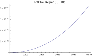
(a) $y+R_{10,10}\left(1/y\right)$

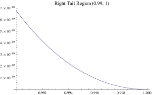
(b) $y+R_{10,10}\left(1/y\right)$

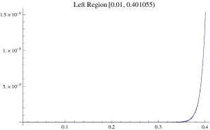
(c) $R_{12,12}\left(z-z_{0}\right)$

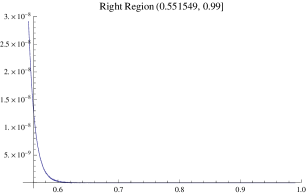
(d) $R_{12,12}\left(z-z_{0}\right)$

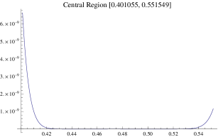
(e) $R_{11,11}\left(u-u_{0}\right)$

Figure 6.1: Algorithm 1 (Padé Approximants): Error Plots $\left|u-F\left(Q_{A}\left(u\right)\right)\right|$.

Despite meeting the accuracy requirements for the given set of parameters, as can be seen from figure 6.1 the error curve produced by this algorithm is far from optimal in the minimax sense. Thus our next two algorithms have to do with constructing so called near best approximants, which are often good enough in practice due to the difficulties involved in finding $R_{m,n}^{*}$. To this end consider the partition $\tau_{L}<u_{1}<u_{2}<1-\tau_{R}$. For simplicity we choose $\tau_{L}=\tau_{R}=10^{-10}$. We are interested in the problem of constructing the Chebyshev series expansions of the functions $A_{L}\left(z\left(u\right)\right)$, $Q\left(u\right)$ and $A_{R}\left(z\left(u\right)\right)$ restricted to the sets $\left[\tau,u\right]$, $\left[u_{1},u_{2}\right]$ and $\left[u_{2},1-\tau_{R}\right]$ respectively. In each case we introduce a linear change of variable $x$ which maps the restricted domain onto the set $\left[-1,1\right]$. To ease notation let $g\left(x\right):=\left.Q\right|_{\left[u_{1},u_{2}\right]}\left(x\right)$; in this case $\left.x\right|\left[u_{1},u_{2}\right]\rightarrow\left[-1,1\right]$ is defined by,

$$x\left(u\right)=\frac{u-\frac{1}{2}(u_{2}+u_{1})}{\frac{1}{2}(u_{2}-u_{1})}=\frac{u-p_{m}}{\bar{r}}.$$ (6.2)

Following from the properties of $Q$, the function $g$ is continuous and of bounded total variation and thus admits the expansion,

$$g\left(x\right)=\frac{\tilde{g}_{0}}{2}+\sum_{k=0}^{\infty}\tilde{g}_{k}T_{k}\left(x\right),\quad x\in\left(0,1\right),$$ (6.3)

where $T_{k}\left(x\right)$ are the Chebyshev polynomials of the first kind and the coefficients $c_{k}$ are defined by,

$$\tilde{g}_{k}=\frac{2}{\pi}\int_{-1}^{1}g\left(x\right)\frac{T_{k}\left(x\right)}{\sqrt{1-x^{2}}}dx.$$ (6.4)

Since the quantile functions $Q$ we have considered in this report are assumed to be infinitely differentiable, elementary Fourier theory tells us that the error made in truncating the series (6.3) after $K$ terms goes to zero more rapidly than any finite power of $1/K$ as $K\rightarrow\infty$, [18, § 3]. Such rapid decrease of the remainder motivates us to seek efficient methods to evaluate the integral in (6.4). This task can rarely be performed analytically so the the usual process is to write (6.4) as,

$$\tilde{g}_{k}=\frac{2}{\pi}\int_{0}^{\pi}g\left(\cos\theta\right)\cos k\theta d\theta,$$

and apply a variant of the fast Fourier transform [21, § 29.3]. This method however would require several thousand evaluations of the function $g$ and result in unacceptable setup times. Fortunately an alternative approach is provided by Thacher [45]. Let the Taylor series expansion of $g$ be given by,

$$g\left(x\right)=\sum_{k=0}^{\infty}g_{k}x^{k}.$$ (6.5)

Then by inverting (6.2) and substituting into (6.1) we see that the coefficients appearing in (6.5) may be written as $g_{k}=\bar{r}q_{k}$. Now substituting the following relationship between the monomials $x^{k}$ and the Chebyshev polynomials [45, eq. 4],

$$x^{k}=T_{0}\left(x\right)+\sum_{j=1}^{k}\theta_{k,j}T_{j}\left(x\right),$$

where,

$$\theta_{j,k}=\begin{cases}2^{1-j}\binom{j}{\frac{j-k}{2}}&j-k\;\textrm{even}\\ 0&j-k\;\textrm{odd}\end{cases},$$

into (6.5), one may express the Chebyshev coefficients $\tilde{g}_{k}$ in terms of the Taylor coefficients $g_{k}$ as follows,

$$\tilde{g}_{k}=\sum_{j=k}^{\infty}g_{j}\theta_{j,k},$$ (6.6)

Thacher’s approach was simple, he observed that applying Shank’s transform to (6.6) one may approximate the Chebyshev coefficients even for slowly convergent series. In our experimentation we found Levin’s $u$-transform to also be affective, which of course was not discovered at the time Thacher wrote his paper. Note that Levin’s $u$ transform has been reported in many instances to outperform Shank’s transform [41]. For efficient Fortran and C++ implementations of these two transforms see [46] and [35] respectively. Thus given the knowledge of the Taylor coefficients $g_{k}$ we now have a method to approximate the Chebyshev coefficients without having to resort to the computationally expensive task of evaluating (6.4) through numerical quadrature. An estimate of the error made in truncating the series (6.3) is given by the magnitude of the first neglected term. In a similar fashion we can construct Chebyshev series expansions for the restrictions $\left.A_{L}\right|_{\left[\tau_{L},u_{1}\right]}$ and $\left.A_{R}\right|_{\left[u_{2},1-\tau_{R}\right]}$. As can be seen from figure 6.2 an algorithm based on constructing truncated Chebyshev expansions in this manner provides us with a much more satisfactory error curve.

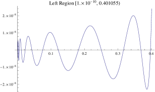
(a) $T_{34,0}\left(x\right)$

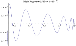
(b) $T_{35,0}\left(x\right)$

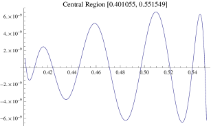
(c) $T_{7,0}\left(x\right)$

Figure 6.2: Algorithm 2 (Truncated Chebyshev Series): Error Plots $\left(Q\left(u\right)-Q_{A}\left(u\right)\right)$

Perhaps the greatest drawback of this algorithm is that it requires one to compute a large number of Chebyshev coefficients. In our example the series needed to be truncated at the $35^{\textrm{th}}$ term in order to satisfy the accuracy requirements in the right region, see figure 6.2. We stress that approximating these $35$ coefficients via 6.6 is not a computationally expensive task in contrast to a numerical integration scheme, however evaluating a $35^{\textrm{th}}$ degree polynomial may lead to unacceptable execution times. It is for this reason we consider constructing Chebyshev-Padé approximants of the function $g$, which are rational functions of the form,

$$T_{m,n}\left(x\right):=\frac{a_{0}T_{0}\left(x\right)+\cdots+a_{m}T_{m}\left(x\right)}{b_{0}T_{0}\left(x\right)+\cdots+b_{n}T_{n}\left(x\right)},$$ (6.7)

which have a formal Chebyshev series expansion in agreement with (6.3) up to and including the term $\tilde{g}_{m+n}T_{m+n}\left(x\right)$. Given the knowledge of the first $n+m+1$ Chebyshev coefficients $\tilde{g}_{0},\ldots,\tilde{g}_{n+m}$, an efficient way to construct $T_{m,n}\left(x\right)$ is to employ the algorithm of Sidi [3], in which the coefficients appearing in 6.7 are computed recursively. For an estimate of the error given by (6.7) see [37, eq. 7.6-12]. Applying this scheme to the same test case as above we obtain the error plots given in figure (6.3).

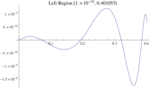
(a) $T_{4,4}\left(x\right)$

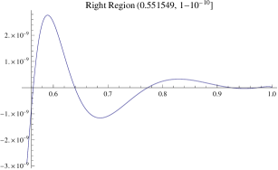
(b) $T_{6,6}\left(x\right)$

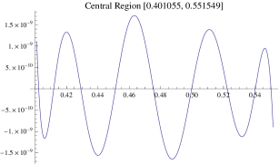
(c) $T_{4,4}\left(x\right)$

Figure 6.3: Algorithm 3 (Chebyshev-Padé Approximants ): Error Plots $\left(Q\left(u\right)-Q_{A}\left(u\right)\right)$

The real benefit of this algorithm is the fast setup and execution times it provides. For example we required a truncated Chebyshev series of degree $34$ to approximate the hyperbolic quantile to the required accuracy in the left region of our test case, again see figure (6.2). On the other hand a Chebyshev-Padé approximant of degree only $8$ provides us with a much better approximant in the same region, contrast with figure (6.3).

Our final algorithm is based on multipoint Padé approximants [26]. Consider the partition $\tau_{L}<p_{m}<1-\tau_{R}$, where $p_{m}$ is the mode location. Choose the points $u_{0},\ldots,u_{K}\in\left[\tau_{L},p_{m}\right]$, and let $s_{0},\ldots,s_{K}\in\mathbb{N}$. Suppose now we want to build a rational approximant $R_{m,n}$ valid on $\left[\tau_{L},p_{m}\right]$ which satisfies the following conditions,

$$A_{L}^{\left(j\right)}\left(z_{k}\right)=R_{m,n}^{\left(j\right)}\left(z_{k}\right),\quad 0\leq k\leq K,\;0\leq j\leq s_{k}-1,$$ (6.8)

where $z_{k}=Q_{B}\left(u_{k}\right)$. Such a problem is called an osculatory rational interpolation problem. The interpolation data on the right hand side of (6.8) may be generated by solving the recycling equation (1.5) for $A_{L}$ with initial conditions imposed at the points $u_{0},\ldots,u_{K}$. Provided a solution to the problem exists it may be solved efficiently through the generalized Q.D. algorithm [34]. This algorithm generates the partial numerators and denominators of a continued fraction, who’s convergents are rational functions called multipoint Padé approximants satisfying (6.8). Similarly by considering solutions to $A_{R}$ we may find a rational approximant valid on $\left[p_{m},1-\tau_{R}\right]$. By choosing only $3$ interpolation points, we apply the method to our test case and provide the results in figure (6.4).

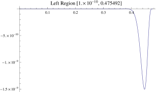
(a) $R_{10,10}\left(z\right)$. Interpolation Data: $u_{0}=p_{m}/3$, $u_{1}=p_{m}$, $s_{0}=15$, $s_{1}=6$

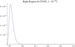
(b) $R_{10,10}\left(z\right)$. Interpolation Data: $u_{0}=p_{m}$, $u_{1}=\left(2+p_{m}\right)/3$, $s_{0}=5$, $s_{1}=16$

Figure 6.4: Algorithm 4 (Multipoint Padé Approximants): Error Plots $u-F\left(Q_{A}\left(u\right)\right)$

One could go a step further and attempt to construct the minimax approximant $R_{m,n}^{*}$, however as mentioned most of the methods known to the present author to construct $R_{m,n}^{*}$ require evaluating $Q$ at a large number of points. It is for this reason we recommend Maehly’s indirect method [31]. This method of constructing $R_{m,n}^{*}$ is applicable when a sufficiently accurate approximation of $Q$ is available. Such an initial approximation may be obtained by the methods described above. Maehly’s indirect method then seeks to find a more optimal approximation in the Chebyshev sense without the need to evaluate $Q$, which of course in our case is an expensive operation. Thus one would expect reduced setup up times with this approach, however we have not explored this idea further.

References

- [1] Peter J. Acklam. An algorithm for computing the inverse normal cumulative distribution function. http://home.online.no/~pjacklam/notes/invnorm/, February 2009.
- [2] Ruben Aldrovandi. Special matrices of mathematical physics: stochastic, circulant, and Bell matrices. World Scientific, 2001.
- [3] Sidi Avram. Computation of the Chebyshev-Padé table. Journal of Computational and Applied Mathematics, 1(2):69–71, June 1975.
- [4] R. Barrio, F. Blesa, and M. Lara. VSVO formulation of the taylor method for the numerical solution of ODEs. Computers & Mathematics with Applications, 50(1–2):93–111, July 2005.
- [5] Carl M. Bender and Steven A. Orszag. Advanced mathematical methods for scientists and engineers: Asymptotic methods and perturbation theory. Springer, 1978.
- [6] N. H. Bingham and R. Kiesel. Modelling asset returns with hyperbolic distributions. Return Distributions in Finance, page 1–20, 2001.
- [7] R. P. Brent and H. T. Kung. Fast algorithms for manipulating formal power series. J. ACM, 25(4):581–595, October 1978.
- [8] N. G. de Bruijn. Asymptotic methods in analysis. Courier Dover Publications, 1981.
- [9] Y. F Chang and G. Corliss. Ratio-Like and recurrence relation tests for convergence of series. IMA Journal of Applied Mathematics, 25(4):349–359, June 1980.
- [10] George Corliss and Y. F. Chang. Solving ordinary differential equations using taylor series. ACM Trans. Math. Softw., 8(2):114–144, June 1982.
- [11] E. A. Cornish and R. A. Fisher. Moments and cumulants in the specification of distributions. Revue de l’Institut International de Statistique / Review of the International Statistical Institute, 5(4):307–320, January 1938. ArticleType: research-article / Full publication date: Jan., 1938 / Copyright © 1938 International Statistical Institute (ISI).
- [12] Germund Dahlquist and Åke Björck. Numerical Methods in Scientific Computing: Volume 1. Society for Industrial Mathematics, September 2008.
- [13] E. De Recherche, Et En Automatique, Domaine De Voluceau, Bruno Salvy, Bruno Salvy, John Shackell, and John Shackell. Asymptotic expansions of functional inverses. 1992.
- [14] G. Derflinger, W. H\örmann, and J. Leydold. Random variate generation by numerical inversion when only the density is known. ACM Transactions on Modeling and Computer Simulation (TOMACS), 20(4):18, 2010.
- [15] G. Derflinger, W. H\örmann, J. Leydold, and H. Sak. Efficient numerical inversion for financial simulations. Monte Carlo and Quasi-Monte Carlo Methods 2008, page 297–304, 2009.
- [16] Ernst Eberlein and Ulrich Keller. Hyperbolic distributions in finance. Bernoulli, 1(3):281–299, 1995. ArticleType: research-article / Full publication date: Sep., 1995 / Copyright © 1995 International Statistical Institute (ISI) and Bernoulli Society for Mathematical Statistics and Probability.
- [17] Ronald A. Fisher and E. A. Cornish. The percentile points of distributions having known cumulants. Technometrics, 2(2):209–225, May 1960. ArticleType: research-article / Full publication date: May, 1960 / Copyright © 1960 American Statistical Association and American Society for Quality.
- [18] David Gottlieb and Steven A. Orszag. Numerical Analysis of Spectral Methods: Theory and Applications. SIAM, 1977.
- [19] Ernst Hairer, Syvert Paul Nørsett, and Gerhard Wanner. Solving ordinary differential equations: Nonstiff problems. Springer, 1993.
- [20] HJ Halin. The applicability of taylor series methods in simulation. In Summer Computer Simulation Conference, 15 th, Vancouver, Canada, page 1032–1076, 1983.
- [21] Richard W. Hamming and Richard Wesley Hamming. Numerical methods for scientists and engineers. Courier Dover Publications, 1973.
- [22] Peter Henrici. Applied and Computational Complex Analysis: Power series. Wiley, 1974.
- [23] G. W. Hill. Generalized asymptotic expansions of Cornish-Fisher type. The Annals of Mathematical Statistics, 39(4):1264–1273, August 1968. Mathematical Reviews number (MathSciNet): MR226762; Zentralblatt MATH identifier: 0162.22404.
- [24] S. R Jaschke. The Cornish-Fisher expansion in the context of delta-gamma-normal approximations. Journal of Risk, 4:33–52, 2002.
- [25] Àngel Jorba. A software package for the numerical integration of ODEs by means of High-Order taylor methods. Experimental Mathematics, 14(1):99–117, 2005. Mathematical Reviews number (MathSciNet): MR2146523; Zentralblatt MATH identifier: 1108.65072.
- [26] George A. Baker Jr and Peter Graves-Morris. Padé Approximants. Cambridge University Press, 2 edition, March 2010.
- [27] Knuth. The Art Of Computer Programming, Volume 2: Seminumerical Algorithms, 3/E. Pearson Education, September 1998.
- [28] G. Leobacher and F. Pillichshammer. A method for approximate inversion of the hyperbolic CDF. Computing, 69(4):291–303, December 2002.
- [29] Eugene Lukacs. Characteristic functions. Griffin, London, 1970. Accessed from http://nla.gov.au/nla.cat-vn1031042.
- [30] Dilip B. Madan and Eugene Seneta. The variance gamma (V.G.) model for share market returns. The Journal of Business, 63(4):511–524, October 1990. ArticleType: research-article / Full publication date: Oct., 1990 / Copyright © 1990 The University of Chicago Press.
- [31] Hans J. Maehly. Methods for fitting rational approximations, parts II and III. J. ACM, 10(3):257–277, July 1963.
- [32] B. Moro. The full monte. Risk Magazine, 8(2):202–232, 1995.
- [33] Frank W. J. Olver, Daniel W. Lozier, and Ronald F. Boisvert. NIST Handbook of Mathematical Functions. Cambridge University Press, May 2010.
- [34] Graves-Morris P.R. A generalised Q.D. algorithm. Journal of Computational and Applied Mathematics, 6(3):247–249, September 1980.
- [35] William H. Press. Numerical recipes: the art of scientific computing. Cambridge University Press, 2007.
- [36] Anthony Ralston. Rational chebyshev approximation by remes’ algorithms. Numerische Mathematik, 7:322–330, August 1965.
- [37] Anthony Ralston and Philip Rabinowitz. A first course in numerical analysis. Courier Dover Publications, 2001.
- [38] Dhiranjan Roy, Ranjan Bhattacharya, and Siddhartha Bhowmick. Rational approximants using Levin-Weniger transforms. Computer Physics Communications, 93(2-3):159–178, February 1996.
- [39] Gennady Samorodnitsky and Murad S. Taqqu. Stable non-Gaussian random processes: stochastic models with infinite variance. Chapman & Hall, June 1994.
- [40] William T Shaw and Nick Brickman. Quantile mechanics II: changes of variables in monte carlo methods and a GPU-Optimized normal quantile. http://econpapers.repec.org/paper/arxpapers/0901.0638.htm, August 2010.
- [41] David A. Smith and William F. Ford. Numerical comparisons of nonlinear convergence accelerators. Mathematics of Computation, 38(158):481–499, April 1982. ArticleType: research-article / Full publication date: Apr., 1982 / Copyright © 1982 American Mathematical Society.
- [42] György Steinbrecher and William Shaw. Quantile mechanics. European Journal of Applied Mathematics, 19:87–112, 2008. 02.
- [43] S. Stoyanov and B. Racheva-Iotova. Numerical methods for stable modeling in financial risk management. Handbook of Computational and Numerical Methods, S. Rachev (ed). Birkh\äuser: Boston, 2004.
- [44] A. Takemura. Orthogonal expansion of the quantile function and components of the Shapiro-Francia statistic. Ann, Statist, 1983.
- [45] Henry C. Thacher,Jr. Conversion of a power to a series of chebyshev polynomials. Commun. ACM, 7(3):181–182, March 1964.
- [46] Ernst Joachim Weniger. Nonlinear sequence transformations: Computational tools for the acceleration of convergence and the summation of divergent series. arXiv:math/0107080, July 2001.
- [47] Ernst Joachim Weniger. Nonlinear sequence transformations for the acceleration of convergence and the summation of divergent series. arXiv:math/0306302, June 2003. Computer Physics Reports Vol. 10, 189 - 371 (1989).
- [48] R. Weron. Computationally intensive value at risk calculations. Handbook of Computational Statistics, Springer, Berlin, page 911–950, 2004.
- [49] A. Zoghbi and I. Stojmenović. Fast algorithms for genegrating integer partitions. International journal of computer mathematics, 70(2):319–332, 1998.
- [50] V. M. Zolotarev. One-dimensional stable distributions. American Mathematical Soc., 1986.