Charge Conjugation, Heavy Ions, $e^{+}e^{-}$ pairs: Was there a better way to add potentials to Dirac’s free electrons?

Abstract

This is a study of a possible alternative procedure for adding a potential energy to the free electron Dirac equation. When Dirac added potentials to his free electron equation, there were two alternatives (here called D1 and D2). He chose D1 and lost charge conjugation symmetry, found Ehrenfest equations that depended on the sign of the energy of the state determining the expectation value, encountered Klein tunneling, zitterbewegung and the Klein paradox. The $D1$ alternative also predicted that deep potentials should pull positive energy states down into the negative energy continuum, possibly creating an unstable vacuum. Extensive experiments (1975-1997) found no evidence for this instability, but did find low energy electron-positron pairs with sharply defined energies and unusually low counting statistics. These pairs tended to disappear with higher beam currents. This paper explores the other alternative, here called $D2$ and finds charge conjugation symmetry preserved, Ehrenfest equations are classical, Klein tunneling is not present, unstable vacuua are forbidden, zitterbewegung is absent in the charge current density, new excitations of bound electron-positron pairs are possible in atoms, and the energies at which low energy electron-positron pair production in heavy ion scattering occurs is well described. Also all of the positive energy calculations, including those with the Coulomb potential, the hydrogen-like atom, are retained exactly the same as found in alternative $D1$. It might have been better if Dirac had chosen alternative $D2$.

I Introduction

In the period 1973-1999 there was considerable activity seeking to use the attractive potential of two heavy ions scattering to pull down the lowest bound state electron states of the two nucleon system down through the mass gap $(-m,m)$ , (here $c=1$), into the negative continuum states. The ideaRafelski et al. (1978); Reinhardt et al. (1981); Greiner and Hamilton (1980) was to destabilize the Dirac Sea by bringing an electron state into contact with the negative energy states. The possibility of making the vacuum unstable generated a great deal of theoretical and experimental excitement which was documented in three conference proceedingsGreiner (1983, 1987); Fried and Muller (1990). The electronic Dirac equation seemed to predict fascinating physics if the positive energy bound states could be pulled down into the negative continuum.

However, after many experiments the only surprising observationGreiner (1983, 1987); Fried and Muller (1990) was the existence of a very narrowly defined total energy peak for an electron-positron pair at a low energy of hundreds of $KeVs$. The best theory had predicted that there should be a dependence on the total charge $Z_{1}+Z_{2}$ of the two heavy nuclei and that there should be a critical threshold for this sum. Above this critical sum there should be evidence of vacuum instability and nothing exceptional should be observed below this threshold. In fact, the electron-positron sum energies for various heavy ion pairs did not correlate well with the nuclear charges and sub-critical pairsBerdermann (1987) also displayed the sharply peaked total energy $e^{-}e^{+}$ pairs.

The early experiments were capable of detecting only one member of the electron-positron pair, but as the experiments grew in sophistication, detection of both members of the pair was possible and the narrowness of the total energy distribution was verified. The mysterious source of these $e^{-}e^{+}$ was apparently generated in the collisions and moved at a slow speed from the scattering center. The counts for these $e^{-}e^{+}$ pairs were generally not very large. They were difficult to detect and it took very long runs to generate good statistics.

A collaboration called APEXape (1989) was organized through Argonne National Laboratory to use the ATLASBollinger (1993) heavy ion accelerator, which was capable of large ion currents, and to use specially developed spectrometers for detecting simultaneously the electrons and positrons from the collisions. The hope was to use the larger currents to lower run times for generating adequate statistics. The early runsBetts (1994) at low beam currents generated fairly convincing data that a sharp total energy peak was present, though the counting statistics were low.

However, as the beam current was increased, the peak did not grow out of the background, rather it seemed to disappear as the run proceeded. The properly skeptical experimentalists decided that the failure of the sharp peak to survive large beam currents and long running times indicated it was an artifact, an unexplained, unreliable chimeraAhmad and APEX (1995),Ahmad and APEX (1997),Ahmad and APEX (1999). Despite reasonable objectionsZeller et al. (1997), the APEX results essentially closed down research in this whole area. There have been almost no papers on this subject since 1999.

What could have gone wrong? The Dirac equation for deep square wells predicts that bound state energy levels can be pulled below the bottom of the mass gap. Yet no vacuum instability was observed. None of a great variety of theoretical ideas could predict the low energy, sharply defined total energy $e^{-}e^{+}$ peaks. Also none of the theories could explain either the wide spread observation of these $e^{-}e^{+}$ pairs for many heavy ion pairs at low beam currents or the disappearance of the sharp peak as the beam current increased. What could be the reason that the efforts of so many capable scientists were not able to confirm the predictions and explain the sharp $e^{-}e^{+}$ peaks?

A very large number of theoretical ideas have been explored hoping to explain these failures. So far it appears that no one has gone back to the beginning of relativistic quantum mechanics and considered the process that Dirac used to add in the potentials to the free electron theory. Before Dirac added in the potential energy, his free electron equation had charge conjugation invariance and the equations of motion of the expectation values obeyed the Ehrenfest classical equations.

The goal of this study is to re-examine Dirac’s derivationDirac (1928),Dirac (1935) of his equations and the way he included a potential energy in his free electron equation. The possibility that there may have been a alternative ”path not taken”Untermeyer (1977) is explored and this possibility seems to recover much of Dirac’s results, resolves the above issues and also points to new physics that may have been excluded by Dirac’s derivation.  In the following, the path taken by Dirac will be labeled $D1$ and the other alternative will be labeled $D2.$  Before delineating these alternatives, it is useful to summarize some of the theoretical consequences of alternative $D1.$

I.1 Consequences of Dirac’s Choice for Incorporating Potential Energy

The non-interacting Dirac equation has an energy spectrum symmetric about zero energy and the equation obeys charge conjugation invarianceMerzbacher (2005),Bjorken and Drell (1964). That is, the negative energy solutions are mapped onto the positive energy solutions and vice versa.  Yet, when a 4-vector potential $A_{\mu}$ is included using alternative $D1$, the charge conjugation invariance breaks down and the energy spectrum is no longer symmetric about zero energy.

The sign of the vector potential is seen to change as the charge conjugation transformation is applied to solutions of the interacting Dirac equation. This has long been interpreted to mean that the positrons, which are represented by the transformed wave functions $\psi_{c}$ have the opposite charge to that of the electronsDirac (1935),Merzbacher (2005),Bjorken and Drell (1964). However, the sign of the positron was originally assigned by looking at the change in the charge of the Dirac vacuum in the absence of a negative electron. This assignment of charge is valid even in the non-interacting Dirac equation where there is no vector potential or explicit charge in the Hamiltonian. This observation would support the argument that the sign change in the vector potential in the transformed Dirac equation could simply be interpreted as evidence that the charge conjugation invariance of the Dirac equation breaks down. The interpretation of the charge of a hole in the vacuum and its positive energy relative to the vacuum is independent of the charge conjugation transformation itself.

In the $D1$ alternative, Dirac’s original approach, which so strongly informs our intuition, we have an apparently consistent theory of electrons and positrons, even though there are some inconsistencies: (1) failing to be charge conjugation invariant in the presence of a vector potential, (2) having Ehrenfest equations of motion for expectation values that depend on the sign of the energy of the wave function forming the expectation value, and (3) having the existence of Klein tunneling in which low energy electrons appear to tunnel into high and wide potential steps that are higher than the mass gap of $2m$. Finally, the perplexing failure of the heavy ion scattering program to discover an unstable vacuum and the appearance of narrowly defined total energy of $e^{-}e^{+}$ pairs, which seem to disappear at high beam currents, suggest that the $D1$ alternative could be inconsistent with nature.

The Ehrenfest theorem, that the equations of motion of expectation values of various operators should reproduce the classical equations of motionMerzbacher (2005); Bjorken and Drell (1964), has long been a limiting check on the validity of quantum mechanical theories.  Derivations in the alternative $D1$ of the equation of motion for the canonical momentum for a particle (electrons with negative charge) in an electric and magnetic field from the interacting Dirac equation ends up with the sign of the Lorentz force law depending on the sign of the energy of the state being used to determine the expectation value of the canonical momentumMerzbacher (2005).

A similar $D1$ derivation from the interacting Dirac equation of the motion of a spin in a magnetic field shows that the direction of the torque on the spin again depends on the sign of the energy of the state being used to calculate the expectation of the spin componentsMerzbacher (2005).  Both of these results contradict the Ehrenfest theorem that the equations of motion for the expectation values should be classical.

Similarly, the probability current density in $D1$ should be a constant in the limit of no electric field, but it remains time dependent in the free particle limit while the momentum remains constant. This also represents a violation of the classical limit of an Ehrenfest equation. The probability current density also exhibits zitterbewegung oscillations at high frequencies of $2m$.

The Klein paradoxBjorken and Drell (1964),Klein (1928) has disclosed a further complication with the interacting Dirac equation in the $D1$ alternative.  There have been a wide variety of demonstrations that something strange occurs if a potential step is too large in energy. Recently, DragomanDragoman (2009) and BowenBowen have noted that the traditional view of the Klein paradox, that the reflection and transmission coefficients are not positive, is easily resolved analytically, but the Klein tunneling remains unresolved.

Finally, combining these theoretical observations of the breakdown of charge conjugation invariance, defective Ehrenfest equations of motion, and Klein tunneling, with the experimental failure to observe a straight forward prediction of vacuum instability and the lack of a theory for the sharp $e^{-}e^{+}$ pairs, argues that a second look at Dirac’s procedure for adding in the potentials should be undertaken.

The rest of the paper is organized as follows:  In section II the two alternative approaches to relativistic quantum mechanics will be delineated with the following:

1. Review of Dirac’s free particle equation and its solutions.

2. Addition of the potential energy to the free electron equation and description of the $D1$ and $D2$ alternatives.

Section III presents several topics comparing the alternatives $D1$ and $D2$ in the following sub-sections.

1. Charge conjugation invariance survives the addition of vector potentials n $D2$, while it fails in $D1$.

2. Ehrenfest equations deficiencies in $D1$ and resolution of these in $D2$.

3. Effect of different one electron states used in $D1$ and $D2$.

4. Bound states in the mass gap in $D1$ and $D2$.

5. Differences between $D1$ and $D2$ for piecewise constant potentials.

6. Klein tunneling in $D1$ and $D2$.

7. Proof by contradiction of a limit for attractive potentials in $D2$.

8. Aspects of Dirac hole theory in both alternatives.

9. Probabililty current density and zitterbewegung in $D1$.

10. Charge current density and the absence of zitterbewegung in $D2$.

11. Completeness in $D2$.

12. Transformations and Feynman Stuckleberg theory in $D1$ and $D2$.

13. Feynman diagrams and Perturbation Theory in $D2$.

Section IV compares the consequences of $D2$ and Heavy Ion Experimental Data with the following subsections:

1. Historical Introduction

2. Hydrogenic Bound states in the Mass Gap

3. Decay modes for bound $e^{-}e^{+}$ metastable states

4. Cross section as a function of energy

5. Free $e^{-}e^{+}$ energies in the Ion Center of Mass Frame

6. Free $e^{-}e^{+}$ energies transformed to the Lab Frame

7. Comparison between Experimental Peaks and bound $e^{-}e^{+}$ metastable transitions

8. Explanation of Tables 1 and 2

Section V is a summary which is followed by two appendices deriving Ehrenfest equations and one discussing induced metastable state decays.

II Describing the two alternatives

In this section the motivation for the $D2$ alternative and its distinction from $D1$ is delineated.

II.1 Free Particle Equations

DiracDirac (1935) sought matrices $\bm{\alpha}$ and $\beta$ so that the free particle Hamiltonian could be written ($c=1$ and $\hbar=1)$ for momentum $\bm{p}$ and mass $m$ as

$$H_{0}=\bm{\alpha}\cdot\bm{p}+\beta m.$$ (1)

The eigenstates of this Hamiltonian were of two types: positive energy $u(\bm{p})$ and negative energy $v(\bm{p})$ and each of these satisfied the equations

$$(\bm{\alpha}\cdot\bm{p}+\beta\mit m)\mit u(\bm{p})=\mit E_{\bm{p}}\mit u(\bm{p}),$$ (2)

$$(\bm{\alpha}\cdot\bm{p}+\beta\mit m)\mit v(\bm{p})=-\mit E_{\bm{p}}\mit v(\bm{p}),$$ (3)

and where

$$\mit E_{\bm{p}}=\sqrt{\bm{p^{2}}+\mit m^{2}}.$$ (4)

One of the most important ideas that Dirac discovered was the charge conjugation symmetry that connected these two eigenvectors to each other and enabled an understanding of the positron.  To briefly review this symmetry, one takes the negative energy eigenvalue equation and changes $\bm{p}\rightarrow-\bm{p}$ and takes the complex conjugate of the equationMerzbacher (2005).  This yields

$$(-\bm{\alpha}^{\ast}\cdot\bm{p}+\beta^{\ast}\mit m)\mit v^{\ast}(-\bm{p})=-\mit E_{\bm{p}}\mit v^{\ast}(-\bm{p}),$$ (5)

where use of $E_{\bm{p}}=E_{-\bm{p}}$ has been made and we now seek a matrix $C$ that has the following properties

$$\bm{C}\bm{\alpha}^{\ast}\mit\bm{C}^{-1}=\bm{\alpha}$$ (6)

and

$$\bm{C}\beta^{\ast}\bm{C}^{-1}=-\beta.$$ (7)

Substituting these into Eqn. 5 yields

$$(-\bm{\alpha}\cdot\bm{p}-\beta\mit m)\bm{C}v^{\ast}(-\bm{p})=-\mit E_{\bm{p}}\bm{C}v^{\ast}(-\bm{p}),$$ (8)

which becomes the positive energy eigenvalue equation after factoring out $-1.$  This means that within a phase factor we have the following connection between the two different energy-signed eigenstates

$$u(\bm{p})=\mit\bm{C}v^{\ast}(-\bm{p}).$$ (9)

Thus, the energy spectrum is symmetric about zero.  For every negative energy eigenvector $v(\bm{p})$ at energy $-E_{\bm{p}}$, there is a corresponding positive energy eigenvector at $+E_{\bm{p}}$ which is given by the charge conjugation transformation.  In the next section the extension of these free particle results to include potential energies following Dirac alternative $D1$ and the alternative path $D2$ will be delineated.

II.2 Incorporating Potential Energy

Given the symmetries of the non-interacting Dirac equation, the next question is how to add in a potential energy.  Intuitively, for the positive energy eigenstates the inclusion of a small potential $V$ should have the form

$$E=E_{\bm{p}}+V,$$ (10)

and should give the correct non-relativistic limit as the momentum goes to zero,

$$E=\sqrt{\bm{p}^{2}+\mit m^{2}}+V\approx m+\frac{\bm{p}^{2}}{2m}+V.$$ (11)

For the negative energy eigenstates, there is no clear criterion for choosing the sign of the potential energy to be included.  There are two possibilities that could make sense:

Alternative $D1$: (Dirac’s choice) is simply to add the potential to the negative energy eigenvalue,

$$E=-E_{\bm{p}}+V=-\sqrt{\bm{p}^{2}+\mit m^{2}}+V\approx-m-\frac{\bm{p}^{2}}{2m}+V.$$ (12)

Alternative $D2$: (The path not taken) would add the potential with a negative sign

$$E=-E_{\bm{p}}-V=-\sqrt{\bm{p}^{2}+\mit m^{2}}-V\approx-m-\frac{\bm{p}^{2}}{2m}-V.$$ (13)

At this moment there is actually little to distinguish or justify either alternative.  The first alternative $D1$ is the simplest, applying the same rule to both energy signed eigenvalues.  The $D2$ alternative restores the symmetry about zero energy that the $D1$ alternative seems to destroy.

The $D1$ alternative has already been shown to be relativistically invariant under Lorentz transformations and leads to an immediate proof that the interacting Dirac equation is covariantBjorken and Drell (1964).

Is it possible that the $D2$ alternative can be made in a Lorentz invariant fashion that will allow a proof that the resulting Dirac equation is covariant?  The first step in such a demonstration requires the review of the Casimir projection operators $B_{+}(\bm{p})$ and $B_{-}(\bm{p})$Merzbacher (2005)

$$B_{+}(\bm{p})\mit u(\bm{p})=\mit u(\bm{p}),\;\mit B_{+}(\bm{p})\mit v(\bm{p})=0$$ (14)

and

$$B_{-}(\bm{p})\mit v(\bm{p})=\mit v(\bm{p}),\;\mit B_{-}(\bm{p})\mit u(\bm{p})=0.$$ (15)

The sign of the energy is a Lorentz invariant.  The positive and negative energy states do not mix under Lorentz transformationsBjorken and Drell (1964).  Using these Casimir operators an operator that yields the Lorentz invariant, the sign of the energy, can be written as

$$sgn(\mit E(\bm{p}))=\mit B_{+}(\bm{p})-\mit B_{-}(\bm{p}).$$ (16)

So, a Lorentz invariant way to write the $D2$ alternative is to substitute $sgn(E(\bm{p)})\mit V$ for the potential energy in the Dirac equation.  Then Dirac’s equation with a potential energy would have the form

$$(\bm{\alpha}\cdot\bm{p}+\beta\mit m+sgn(E)V)\psi(\bm{p})=\mit E\psi(\bm{p}),$$ (17)

which results in the positive eigenvalue equation being written as

$$(\bm{\alpha}\cdot\bm{p}+\beta\mit m+V)u(\bm{p})=\mit Eu(\bm{p}),$$ (18)

and the negative energy eigenvalue equation being written as

$$(\bm{\alpha}\cdot\bm{p}+\beta\mit m-V)v(\bm{p})=-\mit Ev(\bm{p}).$$ (19)

If we again apply the charge conjugation transformation, we see that the energy spectrum in the presence of a potential continues to have the symmetry that was present for the free particle solutions. Charge conjugation transformation invariance is restored.

If the more general case of coupling to electromagnetic fields is considered, the minimal coupling interaction for this $D2$ alternative in the Dirac equation should be replaced by

$$p^{\mu}\rightarrow p^{\mu}-sgn(E)eA^{\mu},$$ (20)

where the charge of the electron is $e$ ($e<0$) and we attempt to follow the sign conventions of Bjorkan and DrellBjorken and Drell (1964). Because the $sgn(E)$ is a Lorentz invariant, there is no change in the vector nature of this transformation and the usual proof of covariance carries through automatically.

III Comparisons between $D1$ and $D2$

In this section several properties of both the $D1$ and $D2$ alternatives will be reviewed.  Several rather striking differences will be found and the reader is urged to keep in mind that this comparison will in some cases be jarring to our intuitions, schooled as we are in the $D1$ alternative.

III.1 Charge Conjugation Invariance with potentials in $D2$

The eigenvalue equation for the Dirac Hamiltonian in the $D2$ alternative will now have the form

$$(\bm{\alpha}\cdot(\bm{p}-\mit sgn(E)e\bm{A})+\beta\mit m+sgn(E)e\phi)\psi(\bm{p})=\mit E\psi(\bm{p}).$$ (21)

For a positive energy state we would have

$$(\bm{\alpha}\cdot(\bm{p}-\mit e\bm{A})+\beta\mit m+e\phi)u(\bm{p})=\mit Eu(\bm{p})$$ (22)

and for a negative energy state

$$(\bm{\alpha}\cdot(\bm{p}+\mit e\bm{A})+\beta\mit m-e\phi)v(\bm{p})=-\mit Ev(\bm{p}),$$ (23)

where $u(\bm{p})$ and $v(\bm{p})$ are used to represent the positive and negative energy solutions in the presence of the vector potential $A^{\mu}.$ Notice that the positive energy equation in $D2$ is exactly the same as in $D1$, so, for example, the positive energy hydrogenic solutions with the Coulomb potential will be the same. It may be likely that a reader might confuse alternative $D2$ with an earlier alternative studied by Müller, Rafelski, and SoffMuller et al. (1973). In this Müller alternative the Coulomb potential was assumed to be multiplied by the $\beta$ matrix. For a hydrogenic solution with a Coulomb potential this altered Dirac equation can be solved analytically, but the atomic spectra does not agree with experiment. The alternative $D2$ is completely different from this earlier model. In $D2$ the positive energy hydrogen is completely unchanged and thus all of the atomic states that agree with experiment are recovered.

If we now take the negative energy equation and change $p\rightarrow-p$ and take the complex conjugate we obtain

$$\bm{\alpha}^{\ast}\cdot(-\bm{p}+\mit e\bm{A})+\beta^{\ast}\mit m-e\phi)v^{\ast}(-\bm{p})=-\mit Ev^{\ast}(-\bm{p}).$$ (24)

Looking for a matrix $C$ exactly as before, we obtain

$$(-\bm{\alpha}\cdot(\bm{p}-\mit e\bm{A})-\beta\mit m-e\phi)Cv^{\ast}(-\bm{p})=-\mit ECv^{\ast}(-\bm{p}),$$ (25)

which becomes the positive energy equation after factoring out the $-1$ and we have the charge conjugation relationship as before

$$u(\bm{p})=\mit\bm{C}v^{\ast}(-\bm{p}).$$ (26)

Thus, this $D2$ alternative restores the invariance of the Dirac equation under charge conjugation transformations even in the presence of a vector potential.

III.2 Ehrenfest Equations in $D2$

As discussed in the introduction, the Ehrenfest equations in $D1$ for the classical Lorenz force depended on the sign of the energy of the wave function evaluated in the expectation values. A similar situation transpires for a spin in a constant magnetic field.

The first of these is the calculation of the change in the momentum in the presence of a vector potential and a scalar potential.  In the Dirac $D1$ alternative the derived equation contains the sign of the energy of the eigenstates used to calculate the expectation valuesMerzbacher (2005).  The derivation is outlined in Appendix A

$$sgn(E)\frac{d}{dt}(\langle m\bm{v\rangle})=-e(\bm{E}+\bm{v}\times\bm{B}).$$ (27)

When the minimal coupling for alternative $D2$ is included, a second factor of $sgn(E)$ multiplies the electric and magnetic fields on the right hand side and cancels out the factor on the left hand side.  This recovers the classical Ehrenfest formula for the momentum

$$\frac{d}{dt}(\langle m\bm{v\rangle})=-e(\bm{E}+\bm{v}\times\bm{B}).$$ (28)

In Appendix B a similar calculation for the spin dynamics of an electron in a magnetic field and factor of $sgn(E)$ for the eigenstates forming the expectation value is also found in the same way as for the Lorentz force law in alternative $D1$.  In alternative $D2$ a second factor of $sgn(E)$ is found on the right hand side and the appropriate Ehrenfest equation is recovered. So, $D2$ corrects the inconsistencies of the Ehrenfest equations in $D1$.

III.3 Choice of one electron basis states in $D2$

In both alternatives the matrix elements of the Hamiltonian can be determined relative to any chosen basis set.  The usual approach is to begin with positive energy free electron plane waves.  An equally valid basis set could be derived from eigenstates of hydrogenic atomic states or the eigenstates of any potential. The hydrogenic set of states would be more appropriate for situations involving a nucleus at the origin as found in heavy ion scattering and other atomic problems. In the mass gap this hydrogenic basis will describe the bound states quite well. For energies outside of the mass gap these eigenstates, though derived from a nucleus at the origin could equally well describe scattering waves about the origin as well as other potentials.  At large energies and large distance from the nucleus the hydrogenic states are essentially coulomb scattering states which become approximately plane wave-like at very large distances.  These basis states reflect the dominant influence of the charged nucleus.  If there are other charges, as in scattering from other atoms, it may be desirable to distinguish between the internal potential which gives rise to the hydrogenic states and the external potential that could describe scattering in this basis based on the central nucleus.  In both of the alternatives, the scattering states at high energies and large distances will behave very much like the free electron bases. However, in $D2$ the atomic hydrogenic states will exhibit bound states in both the top and bottom halves of the mass gap because the energy specrum must be symmetric about zero. Electron and positron scattering results should be able to be described by any similar bases. The distinguishing characteristic will be the bound states in the gap.

III.4 Bound States in the Mass Gap in $D1$ and $D2$

When bound states in the mass gap are considered, there are very real differences between the two alternatives.  In alternative $D1$ , there are only bound states in the positive half of the mass gap and no states in the lower half of the mass gap.  In alternative $D2$ the positive energy bound states in the upper part of the mass gap are mapped by the charge conjugation transformation into the lower half of the gap.  The existence of these bound states in the lower half of the mass gap gives rise to a new set of excitations that do not exist in the $D1$ alternative.  These negative energy bound states in the lower part of the gap must also be filled in the Dirac vacuum.  Excitations out of these states will leave behind bound holes in the vacuum that are localized near the nucleus.  The existence of these states should give rise to excitations that were not expected in alternative $D1.$  It should be possible to distinguish between the two alternative by examining the properties of these hole states.  That is the goal of a later section in this paper which examines data from heavy ion scattering experiments mentioned above. $D2$ displays a different energy spectrum in the mass gap from $D1$.

III.5 Piece-wise Constant Potentials in Alternative $D1$ and $D2$

The examination of constant potentials is important because any potential can be approximated mathematically by piecewise constant potentials.  In the following discussion the calculation will be carried out in one dimension for spinless particles since it simplifies the mathematics.  This reduces the matrices to $2\times 2$’s and spinors to $1\times 2$’s.

Consider first a positive constant potential $V_{0}$ in a certain region.  In this region the wave function

$$\psi(z)=ae^{ikz}\biggl{[}\begin{array}[]{c}u_{1}\\ u_{2}\end{array}\biggr{]}$$

will carry a current in the positive $z$ direction.  Now consider a comparison of this wave function and its energy spectrum $E$ in both the $D1$ and $D2$ alternatives.

In alternative $D1$, the Dirac equation yields the following secular matrix equation

$$\biggl{[}\begin{array}[]{cc}V_{0}-E+m&k\\ k&V_{0}-E-m\end{array}\biggr{]}\times\biggl{[}\begin{array}[]{c}u_{1}\\ u_{2}\end{array}\biggr{]}=0.$$

It is easy to show that the energy eigenvalues are

$$E_{k}^{\pm}=V_{0}\pm\sqrt{m^{2}+k^{2}},$$ (29)

and the wave functions are

$$\psi_{k}^{+}(z)=ae^{ikz}\biggl{[}\begin{array}[]{c}1\\ \frac{k}{m+\sqrt{m^{2}+k^{2}}}\end{array}\biggr{]},$$

and

$$\psi_{k}^{-}(z)=ae^{ikz}\biggl{[}\begin{array}[]{c}-k\over(m+\sqrt{m^{2}+k^{2}})\\ 1\end{array}\biggr{]}.$$

The defining signs of the energies are relative to $V_{0}$ and the actual sign of the energy will depend on the size of $V_{0}.$

The ”positive” energy states are found for $E>V_{0}+m$ and the ”negative” energy states are found for $E<V_{0}-m$ and there are no states found in the mass gap $V_{0}-m<E<V_{0}+m$ which is centered on $V_{0}.$  As $V_{0}$ becomes more positive, the ”negative” (relative to $V_{0})$ states are pulled up in energy and can become degenerate with positive energy states in a nearby region, leading to Klein paradox effects.  These effects were shown in Fig. 1 for the energy range $(m,V_{0}-m)$ if $V_{0}$ is large enough.  Specifically, for a potential step of height $V_{0}$ and extending infinitely far in one direction, the transmission coefficient $T$ can be calculated analytically. If the potential step height $V_{0}$ is less than the width of the mass gap, $V_{0}<2m$, (in this section $\hbar=1$ and $c=1$), the transmission coefficient $T$ is zero for incident particle energies $E$ in the range $m<E<V_{0}+m$ and becomes non-zero for $E>V_{0}+m.$  $T$ approaches $1$ as the incident energy becomes large.  These results are very classical.

If the potential step is larger so that $V_{0}>2m,$ the transmission coefficient develops a non-zero value between $m$ and $V_{0}-m.$  It is as if the barrier has become partially transparent to particles in the range $m<E<V_{0}-m.$  Mathematically, this effect is due to the negative energy states (relative to $V_{0})$ being pulled up into degeneracy with the positive energy states of the incident particles.  An example of the transmission coefficient for this case is shown in Fig. 1, for the value of $V_{0}/m=3.$  This situation of Klein tunneling presents a serious challenge for any theory of low energy particles because they would appear to tunnel into high and infinitely wide barriers with very little energy.  This would seem to contradict widely observed classical phenomena.

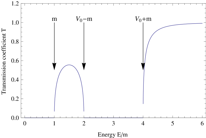
Figure 1: The one dimensional transmission Coefficient $T$ (calculated in alternative D1 ) for a potential step of height $V_{0}/m=3$ for $0<x<\infty$ plotted as a function of the incident particle energy $E$. The small peak between $m<E<V_{0}-m$ is the Klein tunneling.

The situation for the $D2$ alternative is quite different.  The secular matrix equation becomes

$$\biggl{[}\begin{array}[]{cc}sgn(E)V_{0}-E+m&k\\ k&sgn(E)V_{0}-E-m\end{array}\biggr{]}\times\biggl{[}\begin{array}[]{c}u_{1}\\ u_{2}\end{array}\biggr{]}=0$$

and the eigenvalues satisfy

$$sgn(E)(|E|-V_{0})=\pm\sqrt{m^{2}+k^{2}}.$$ (30)

So, for the positive sign the eigenvalue is

$$E_{k}^{+}=V_{0}+\sqrt{m^{2}+k^{2}},$$ (31)

while for the negative sign

$$E_{k}^{-}=-V_{0}-\sqrt{m^{2}+k^{2}}$$ (32)

and the corresponding wave functions are unchanged.

In this $D2$ alternative the positive energy states are found for $E>V_{0}+m$ and the negative energy states are found for $E<-(V_{0}+m).$  There are no oscillatory states allowed in the intervening interval $-(V_{0}+m)<E<V_{0}+m.$  Since there are no states in this interval, there is no possible current in this energy range.  In contrast to the $D1$ alternative, in the $D2$ alternative increasing the strength of the potential simply widens the interval in which no states are allowed.  It is not possible for ”negative” energy states to ever be degenerate with positive energy states in a neighboring region. The $D2$ alternative suppresses the Klein tunneling allowed in $D1$.

III.6 Klein Tunneling in $D1$ and $D2$

Consider the classic step potential of the Klein paradox ($V=0$ for $z<0$ and $V=V_{0}$ for $z>0$ )in the $D2$ alternative. There are no states for $z>0$ in the energy interval $m<E<V_{0}+m,$ and the transmission coefficient $T$ must be zero in this interval.  For energies $E>V_{0}+m$ the transmission coefficient $T$ is given by

$$T=\frac{4r}{(1+r)^{2}},$$ (33)

where

$$r=\sqrt{\frac{E-(V_{0}+m)}{E-(V_{0}-m)}}\sqrt{\frac{E+m}{E-m}}$$ (34)

and $E=\sqrt{m^{2}+k^{2}}$ is the incident energy.

In the $D2$ alternative there is no Klein paradox.  Increasing $V_{0}$ simply expands the interval $(m,V_{0}+m)$ where $T=0.$  If Fig. 1 were constructed in the $D2$ alternative, there would be no small peak between $m$ and $V_{0}-m$ and $T=0$ in that interval.  There is no question about the potential being too strong.  There is simply no current in the step in the energy interval $(m,V_{0}+m).$

In this classic step problem it is possible to find evanescent waves whose energies are less than $V_{0}+m.$  These evanescent waves do not carry currents, so their presence does not change the discussion about $T$ vanishing in the interval $(m,V_{0}+m).$

In the $D2$ alternative the evanescent wave function for $z>0,$ for example, will have the following form

$$\psi(z)=ae^{-\kappa z}\times\biggl{[}\begin{array}[]{c}w_{1}\\ w_{2}\end{array}\biggr{]}$$

and the eigenvalues are found to be

$$E_{\kappa}^{+}=V_{0}+\sqrt{m^{2}-\kappa^{2}}$$ (35)

and

$$E_{\kappa}^{-}=-V_{0}-\sqrt{m^{2}-\kappa^{2}}$$ (36)

where $0<\kappa<m$ and for the positive energy state $w_{1}=1$ and $w_{2}=i\kappa/(m+\sqrt{m^{2}-\kappa^{2}}).$  No states are allowed in the interval $(-V_{0},V_{0}).$  These evanescent states would enable tunneling in the energy interval $(V_{0},V_{0}+m),$ but not in the interval $(-V_{0},V_{0}).$

It should be noted again that the energy spectrum of these states are symmetric about the zero energy. $D2$ does not allow the Klein tunneling effects which are in $D1$.

III.7 Attractive Potentials in $D1$ and $D2$

In $D1$ a negative square well can have any depth. It is possible to have bound states in the gap of such a potential at any depth in the mass gap. It was the question of what happens when the potential is deeper than the mass gap and bound states of this potential were to merge with the continuum of negative states below the mass gap that motivated the unsuccessful search for unstable vacua by Greiner and colleagues.

In $D2$ the presence of $sgn(E)$ gives rise to a surprising difference from $D1$.  Consider a negative potential $V(x)$ (for the moment restrict the potential to be one dimensional).  Consider first a positive energy eigenstate of this system.  This means that the $sgn(E)$ factor multiplying the potential is positive.  For a negative potential the eigenvalues that are lower than $m$ will be found in the mass gap $(-m,m).$  How deep can the potential be and still give rise to a positive energy eigenvalue?  Clearly if the depth of the potential is less than $m$ the bound states will be above zero and will clearly have positive energies.  However, if a potential extends from $+m$ down to some negative energy below zero, it is possible that the potential could have a bound state that is below zero, that is negative, but we have been considering only positive energies and this would lead to a contradiction.  Thus, this reductio ad absurdum argument would imply that in alternative $D2$, a negative potential cannot be deeper than $-m$ or more precisely, cannot have bound states that are below zero energy. Because of the charge conjugation symmetry in $D2$, this would mean that the energy spectrum remains symmetric about zero and the eigenstates and eigenvalues are mapped from positive energy onto negative energies. There cannot be any crossing through zero.

From this perspective it is notable that the positive energy hydrogenic bound states of the Dirac equation are clearly in the interval $(0,m)$ and that the lowest possible state for a nuclear charge $Z$ is zero as $Z\rightarrow 1/\alpha_{0},$ where $\alpha_{0}$ is the fine structure constant.

In this $D2$ alternative a plot of the potential energies for both positive and negative energy states will have a reflection symmetry about zero energy and never cross over the zero energy.  No attractive potential for negative energy states can extend above the zero energy level.  There does not seem to be any such restriction on repulsive potentials since any eigenvalues would be larger than $m.$  There does not seem to be any obvious restriction on the height of barriers.

$D2$ seems to imply that no positive energy state can cross the zero energy line as is allowed in $D1$. This property explains why the search for an unstable vacuum was not successful. The ultimate question is whether nature actually exhibits distinctive behavior that confirms the $D2$ alternative as the correct alternative.

III.8 Hole Theory in $D1$ and $D2$

Let us now consider Dirac’s argument for positrons in the hole theory in both $D1$ and $D2.$  First, it must be re-iterated that in the free electron case there is explicitly no charge in the Hamiltonian.  Charge only enters the description in the presence of a vector potential.  Charge enters into the hole theory in an independent fashion through an argument for the change in charge of the vacuum in the presence of a hole.

In the absence of any potential both $D1$ and $D2$ are the same.  The Dirac vacuum with all of the negative energy states filled is necessary to avoid transitions to unbounded negative energies.  In both alternatives a hole in the free electron vacuum at an energy of $-E_{p,}$ momentum $-p$ , and spin $-s$ is clearly interpreted by the change in the energy of the many electron state as a positive energy state $E_{p,}$ with momentum $p$ and spin $s.$  The charge associated with a hole is imputed by observing the change in the charge of the vacuum plus hole in comparison with the vacuum.  The charge in not carried by the wave function.  The charge is the opposite of whatever the charge was of the original electrons whose wave functions were solutions of the free electron Dirac equation.

$D2$ describes positron wave functions using charge conjugation in the same way as does $D1$. However, the positron wave function in $D2$ is identical with some positive energy electron wave function in contrast to $D1$. The charge is not carried in the wave function, but is ascribed by the change in the vacuum as in $D1$.

In $D1$ there is a long history of ascribing of the charge of the vector potential in the Dirac equation under the charge conjugation transformation as evidence that the positron wave function represents an opposite charge from the electron. From the perspective of $D2$ this sign change is simply the breakdown of charge conjugation invariance in $D1$. In $D2$ the positron wave function must necessarily be identical to a positive energy electron state just as is true for the free electrons. The positron charge is not carried inherently in the wave function and must be imputed separately.

III.9 Current Density and Zitterbewegung in $D1$

A central argument for the $D1$ alternative has been the discussionBjorken and Drell (1964) of the probability current density for free electrons.  The standard derivation for the continuity equation of the probability density yields for the probability current density

$$J_{i}=c\alpha_{i}$$ (37)

where $c$ is the velocity of light and $\alpha_{i}$ is one of the Dirac matrices.

This result has long been regarded as peculiar since in the classical limit we expect the current density to be carried by the momentum $p_{i}/m.$  A long standing puzzle related to this peculiarity is the fact that in the absence of a potential the momentum is a constant of the motion.  However, this probability current density does not commute with the Hamiltonian and is not a constant of the motion in the absence of interaction potentials. This is the third Ehrenfest equation in $D1$ which does not obey the classical limit.

In the $D1$ alternative using a wave packet constructed out of positive energy states

$$\psi_{(+)}(x)=\int\frac{d^{3}p}{(2\pi\hbar)^{3/2}}\sqrt{\frac{m}{E_{p}}}\sum_{s}b(p,s)u(p,s)e^{-ip\cdot x},$$ (38)

it is straight forward to evaluate the expectation value of the probability current density and show that

$$\langle J_{i}\rangle_{+}=\langle c\alpha_{i}\rangle_{+}=\int\frac{d^{3}p}{(2\pi\hbar)^{3/2}}\frac{c^{2}p_{i}}{E_{p}}|b(p,s)|^{2}=\langle\frac{c^{2}p_{i}}{E_{p}}\rangle_{+}$$ (39)

where the subscript $+$ on the averages indicates only the positive energy states are used.

At this point a crucial argument has been made in the $D1$ alternative.  It is noted that the eigenvalues of the $c\alpha_{i}$ matrices are $\pm c$, corresponding to positive and negative energies, and if the expectation value of the probability current density is to be calculated using the eigenvectors of the $\alpha_{i}$ matrices it will require the inclusion of negative energy states in order to obtain a velocity associated with the probability current density less than the velocity of light.

When the current density is evaluated using such a linear combination of states,

$$\psi(x)=\int\frac{d^{3}p}{(2\pi\hbar)^{3/2}}\sqrt{\frac{m}{E_{p}}}\sum_{s}( b(p,s)u(p,s)e^{-ip\cdot x}$$ (40)

$$+d^{\ast}(p,s)v(p,s)e^{ip\cdot x}),$$

the resultBjorken and Drell (1964) is a weighting of the momentum by the amplitudes $|b(p,s)|^{2}$ and $|d(p,s)|^{2},$ and also the famous zitterbewegung terms that exhibit frequencies on the order of the rest mass $\pm 2mc^{2}.$  These high frequency terms have been puzzling and have led to a number of intuitive arguments about confinement and the excitation of electron-positron pairs in the presence of static potentials.

The amplitude of the zitterbewegung in the expectation value of the probability current density is proportional to the amplitude $d^{\ast}(p,s)$ of the negative energy states in the wave function.  The next series of $D1$ arguments are guided by an example wave function.  A typical wave functionBjorken and Drell (1964) at zero time is

$$\psi(x)=(\pi d^{2})^{-3/4}e^{-\frac{x^{2}}{2d^{2}}}w_{1}(0)$$ (41)

where $d$ is the ”confinement width” of the wave function and $w_{1}(0)$ is the spin up spinor for an electron with zero momentum and positive rest energy.

The amplitude of a positive energy plane wave in this state is

$$b(p,s)=A(\frac{d^{2}}{\pi\hbar^{2}})^{3/4}e^{-\frac{p^{2}d^{2}}{2\hbar^{2}}},$$ (42)

and the amplitude for a negative energy state is

$$d^{\ast}(p,s)=A(\frac{d^{2}}{\pi\hbar^{2}})^{3/4}e^{-\frac{p^{2}d^{2}}{2\hbar^{2}}}\frac{pc}{E_{p}+mc^{2}},$$ (43)

where $A$ is a normalization factor.

The relative fraction of the negative energy states in this wave function is small unless $pc\approx mc^{2}$ or greater.  At the same time the confinement of the wave function to a region of size $d$ implies the momentum must be $p\leq\hbar/d,$ or that the confinement is comparable to the Compton wavelength

$$d\approx\frac{\hbar}{mc}.$$ (44)

From these arguments in $D1$ there have evolved two conclusions.  If the confinement of a wavefunction is on  the order of the Compton wavelength or smaller, negative energy states will be significantly probable.  Because of the connection between negative energy states and positrons this would mean that static, confining potentials should generate electron-positron pairs under the conditions of close confinement.

The origin of these arguments in $D1$ is the fact that the probability current density is not proportional to the momentum operator and to get a speed associated with the probability current density to be less than the velocity of light, negative energy states must be mixed into any wave function.  The relevant question, besides the question of whether all of the inconsistencies of $D1$ are acceptable, is whether the probability current density is what transports the charge density.  This question is resolved in $D2$ in the next section.

These ideas are deeply engrained in those of us who have learned quantum mechanics in alternative $D1.$  In particular, we have been forced into these outcomes by the form of the probability current density.  Let us now examine the same picture from the point of view of alternative $D2.$

III.10 Charge Current Density in $D2$

First, it must be noted that both alternatives $D1$ and $D2$ will have the same probability current density for free electrons.  For free electrons there is no distinction between the two alternatives.  However, there is also explicitly no charge in the free electron Hamiltonian. To examine the charge current density it is necessary to examine the Hamiltonian that couples the electrons to a vector potential.

The $D2$ alternative differs primarily in the treatment of the electron equations in the presence of a vector potential $A_{\mu}=(\Phi,A_{i}).$ For a Hamiltonian that couples vector potentials to the free electrons, the charge current density $J_{i}^{Q}$ is most easily derived by

$$J_{i}^{Q}=-\frac{\partial H}{\partial A_{i}}.$$ (45)

Since the Hamiltonian in alternative $D2$ is

$$H=c\bm{\alpha}\cdot\bm{p}+\beta mc^{2}-e\>sgn(E)\bm{\alpha}\cdot\bm{A}+e\>sgn(E)\Phi,$$ (46)

the charge current density is

$$J_{i}^{Q}=esgn(E)\alpha_{i}={\frac{1}{2}}e\>(sgn(E)\alpha_{i}+\alpha_{i}sgn(E)),$$ (47)

where in the second equality the charge current density operator has been symmetrized as needed for the free electron Hamiltonian. For free electrons with momentum $\bm{p}$ , we have that $sgn(E)$ can be represented by a projection operator

$$sgn(E)=\frac{c\bm{\alpha}\cdot\bm{p}+\beta mc^{2}}{E_{p}}.$$ (48)

Substituting the expression for the free electron projection operators into the expression for $J_{i}^{Q}$ we obtain

$$J_{i}^{Q}=e(1/2)(c\bm{\alpha}\cdot\bm{p}\alpha_{i}+c\alpha_{i}\bm{\alpha}\cdot\bm{p}+mc\{{\beta,\alpha_{i}}\})$$ (49)

and using the anti-commutation relations for the $\alpha_{i}$ and $\beta$ matrices

$$\{\alpha_{i},\alpha_{j}\}=2\delta_{i,j}$$ (50)

$$\{\alpha_{i},\beta\}=0$$ (51)

we obtain the current density operator proportional to a component of the momentum operator

$$J_{i}^{Q}=I_{4}ec\frac{p_{i}}{E_{p}},$$ (52)

the matrix $I_{4}$ is the $4x4$ identity matrix and $p_{i}$ is the i-th component of the momentum operator.

Thus, in alternative $D2$ the charge current density is in excellent accord with classical expectations.  It is proportional to the momentum, is a constant of the motion in the absence of a potential, thus satisfying the Ehrenfest equations which were violated in alternative $D1.$  Because the charge current density is proportional to the momentum there is no zitterbewegung! There is no paradox as in $D1$ where the probability current density operator has eigenvalues which force the inclusion of negative energy states in wave packets.  Expectations of the current density can be determined completely by positive energy wave packets as above. There is no necessity for the inclusion of negative energy states in wave function packets as was argued in $D1$. .  In alternative $D2$ the negative energy states are derived from the positive energy states by the charge conjugation transformation and only the positive energy states are necessary for completeness.

The arguments that confinement by static potentials necessarily induces particle anti-particle states in so far as it was based on arguments of eigenvalues of $c\alpha$ no longer has any imperative in alternative $D2.$ In $D2$ the charge current density, which is what describes the movement of the charge, is proportional to the momentum and there is no zitterbewegung or generation of positrons by confinement in static potentials as argued in $D1$.

III.11 Completeness in $D2$

It is often argued in $D1$ that positive energy states are not complete. This argument relies completely on the apparent need in $D1$ for negative energy eigenvalues of the $\alpha$ matrices. As has been discussed above there is no need for this argument when considering the charge current density. In $D2$ the standard mathematical proofs based on the Fourier TheoremMorse and Feshbach (1953) can be used to prove that the positive energy states are complete in the Hilbert space. Since the negative energy states are connected to the positive energy states by the charge conjugation transformation, they are not linearly independent of the positive energy states. This means that the positive energy states are complete and are the only set of states needed. The inferences in $D1$ based on the probability current density and the eigenfunctions of the $\alpha$ matrix are irrelevant to the charge current density and thus the movement of charge in $D2$. The arguments on confining potentials generating $e^{-}e^{+}$ pairs does not arise in $D2$. In $D2$ the positive energy states are complete in contrast to the conclusions in $D1$.

III.12 Transformations and Feynman/Stuckleberg Theory in $D1$ and $D2$

In both of the alternatives $D1$ and $D2$ there are three transformations that can be formulated in the free electron basis.  These transformations are well defined in several referencesBjorken and Drell (1964); Merzbacher (2005); Messiah (1961).  They are: $\bm{C}$ charge conjugation, $\bm{\tau}$ time reversal, $\bm{P}$ parity transformations.  If we write the Hamiltonian in two parts:

$$H_{0}=\bm{\alpha}\cdot\bm{p}+\beta m$$ (53)

and

$$H_{1}=-e\bm{\alpha}\cdot\bm{A}+e\Phi,$$ (54)

it is easy to show the following transformations.

$$\bm{C}H_{0}(\bm{p})\bm{C}^{-1}=-H_{0}(-\bm{p}),$$ (55)

$$\bm{P}H_{0}(\bm{p})\bm{P}^{-1}=H_{0}(-\bm{p}),$$ (56)

$$\bm{\tau}H_{0}(\bm{p})\bm{\tau}^{-1}=-H_{0}(-\bm{p}).$$ (57)

The first of these shows that the free electron Hamiltonian has a reflection symmetry about zero energy and is charge conjugation invariant.   By exactly the same process for free electron states, we can show

$$\bm{C}sgnE(\bm{p})\bm{C}^{-1}=-sgnE(-\bm{p}),$$ (58)

$$\bm{P}sgnE(\bm{p})\bm{P}^{-1}=sgnE(-\bm{p}),$$ (59)

$$\bm{\tau}sgnE(\bm{p})\bm{\tau}^{-1}=-sgnE(-\bm{p}).$$ (60)

If we apply these transformations to the interaction part of the Hamiltonian, we obtain

$$\bm{C}H_{1}\bm{C}^{-1}=H_{1},$$ (61)

$$\bm{P}H_{1}\bm{P}^{-1}=H_{1},$$ (62)

$$\bm{\tau}H_{1}\bm{\tau}^{-1}=H_{1}.$$ (63)

In alternative $D2,$ we have charge conjugation invariance and have the following transformations.

$$\bm{C}(H_{0}(\bm{p})+sgnE(\bm{p})H_{1})\bm{C}^{-1}=-(H_{0}(-\bm{p})+sgnE(-\bm{p})H_{1},$$ (64)

$$\bm{\tau}(H_{0}(p)+sgnE(\bm{p})H_{1})\bm{\tau}^{-1}=-(H_{0}(-\bm{p})+sgnE(-\bm{p})H_{1}).$$ (65)

Negative energy wave functions are transformed into positive energy wave functions and vice versa.  The charge conjugation wave function $\psi_{c}$of a negative energy state $\psi_{(-)}$ is given by

$$\psi_{c}=\bm{C}\psi_{(-)}^{\ast}$$ (66)

is identical with a positive energy state with the appropriate momentum and spin and define the positron wavefunction.  Just as in alternative $D1,$ because the time reversal transformation gives rise to the same transformation properties as for the charge conjugation, the time reversed wave function will necessarily be the same (within multiplication by a constant matrix) as the charge conjugation transformed wave function except for a phase factor. The Wigner time reversed wave function ${\Psi_{PCT}}$ Bjorken and Drell (1964) is an explicit representation of this connection between positron wave functions and a matrix multiplied by the wave function of a negative energy electron moving backward in space time and is valid in $D2$ as well as $D1$.

In alternative $D1$ charge conjugation invariance is broken and we have

$$\bm{C}(H_{0}(\bm{p})+H_{1})\bm{C}^{-1}=-{(H_{0}(-\bm{p})-H}_{1}).$$ (67)

In much of the literature about alternative $D1$ this breakdown of the charge conjugation invariance has been interpreted as evidence for the sign change of the positron.  This has persisted even though the positron charge was determined by the vacuum neutrality condition.  From the perspective of the $D2$ alternative, the change of sign is just the breakdown of charge conjugation invariance.

In $D2$ it is possible to demonstrate the apparent charge difference by examining the negative energy wave function and its time reversal transform. For a positive energy, the wave functions must obey

$$i\hbar\frac{\partial\psi_{(+)}}{\partial t}=(\bm{\alpha}\cdot(\bm{p}-e\bm{A})+\beta m+e\Phi)\psi_{(+)}.$$ (68)

For a negative energy the wave function must obey an equation that looks like an oppositely charge particle, except for having a negative energy.

$$i\hbar\frac{\partial\psi_{(-)}}{\partial t}=(\bm{\alpha}\cdot(\bm{p}+e\bm{A})+\beta m-e\Phi)\psi_{(-)}.$$ (69)

The time inversion transformation identifies the transformation of this negative energy wave function as a positive energy wave function traveling backward in time.

III.13 Feynman Diagrams and Perturbations in $D1$ and $D2$

Because in $D2$ the negative energy states are determined by mapping from the positive energy states using the charge conjugation transformation and the positron amplitude has been identified with negative energy wave functions moving backward in space time, the application of the whole diagrammatic structure of the Feynman Stuckleberg perturbation structureBjorken and Drell (1964) should be exactly the same in $D1$ and $D2$ when applied on positive energy states. The negative energy results could then be obtained by the charge conjugation transformation.

IV Heavy Ion Scattering as evidence for alternative D2

In this section the experimental energies of the sharply defined $e^{-}e^{+}$ pairs seen in heavy ion scattering will be compared with predictions of the $D2$ alternative. The properties of $D2$ delineated in the previous sections already predict that no evidence of an unstable vacuum would be found because positive and negative energy eigenvalues are separated by the zero energy.

IV.1 Historical Introduction

P. A. M. Dirac’s Dirac (1928) proposal for a ”vacuum” in which all of the negative energy electron states were filled has led to a detailed understanding of free positrons, including their production and annihilationBjorken and Drell (1964). However, the extension of his insights to bound, hydrogenic-like atomic states of the Coulomb potential has resulted in a strange story of contradictory experimental and theoretical results.  Using a widely held version of alternative $D1$ and vacuum for bound states Greiner and Hamilton (1980), Greiner and numerous colleaguesRafelski et al. (1978),Reinhardt et al. (1981) proposed a series of compelling effects to be seen in the high electric fields of heavy ion scattering experiments.

These predictions and experiments were the motivation for three international proceedings: LandsteinGreiner (1983) MarateaGreiner (1987) and CargeseFried and Muller (1990).

The 1990 summary lectureMuller (1990) by Müller, for the last international meeting Fried and Muller (1990), assembled a table of $e^{-}e^{+}$ pair sum energies and noted that ”the phenomenology of data was so complex that they do not fit into any simple scheme..” and little hope was offered of finding such a scheme.  An introductory essay for this same conference by J. RafelskiRafelski (1990) ruminated that striking experimental observations were needed showing the breakdown of the vacuum in order to be sure that their understanding not be ”Ptolemean”, that is, making a fundamental mistake in a basic notion, leading to more and more complex descriptions.  None of the theories in this meetingFried and Muller (1990) were able to make sense of the carefully crafted experimental data.

IV.2 Hydrogenic bound $e^{-}e^{+}$ states in the mass gap

The charge conjugation invariance in $D2$ gives rise to a very different structure of states in the mass gap. The positive energy states for the hydrogenic atom are the same in both $D1$ and $D2$. In $D2$ the charge conjugation invariance maps the positive energy bound states to the lower half of the mass gap. Shown in Fig. 2 is a representation of the mass energy gap of the Dirac equation in both the $D1$ and $D2$ alternatives. In each alternative the Dirac vacuum will be formed by assuming all of the negative energy states are occupied by electrons. In the $D2$ alternative that would include the negative energy bound states in the lower part of the gap. Of course, in the $D1$ alternative there are no bound states in the bottom of the gap.

Figure 2: Representation of the types of electron positron excitations available in Alternatives $D1$ and $D2$. The two excitations on the left are available in both $D1$ and $D2$, but the excitation on the right represents a bound $e^{-}e^{+}$ pair that is only possible in alternative $D2$.

The excitations on the left side of Figure 2 are present in both $D1$ and $D2$ because they involve holes below the mass gap. The left most excitation creates a free $e^{-}e^{+}$ pair. The second excitation creates an excited atomic state and a free positron.

The right side of Fig. 2 is only found in the $D2$ alternative and illustrates an excitation from an occupied negative energy bound state to an (unoccupied) positive energy bound state. This state will be described as a bound $e^{-}e^{+}$ pair state.  These bound $e^{-}e^{+}$ pairs within an ion constitute a new excited state of the system.  The movement of these bound $e^{-}e^{+}$ pairs is carried by the ions.  Similarly, vertical excitations during ion-ion collisions from the filled vacuum states to an empty (ionized) positive energy state would give rise to a metastable, bound $e^{-}e^{+}$ pair state on one or both of the scattered ions.

In the following we will argue that these excitations are responsible for the narrowly defined free $e^{-}e^{+}$ pair energies observed in heavy ion scattering. For that argument it is first necessary to determine the excitation energies for these bound $e^{-}e^{+}$ pairs.

In the $D2$ hydrogenic approximation the energy levels of the $e^{-}e^{+}$ bound pairs will be the difference between the positive energy bound hydrogenic state $E_{+}(n,j)$ and the negative energy bound state $E_{-}(n,j)$ where

$$E_{\pm} (n,j)=$$ (70)

$$\pm m\left[1+(\frac{Z\alpha_{0}}{n-(j+\frac{1}{2})+\sqrt{(j+\frac{1}{2})^{2}-(Z\alpha_{0})^{2}}})^{2}\right]^{-\frac{1}{2}}$$

where $Z\alpha_{0}$ is the product of the charge on the nucleus and the fine structure constant.  In the hydrogenic approximation the bound $e^{-}e^{+}$ pair energy difference would be

$$\Delta\epsilon(n,j;n^{\prime},j^{\prime}) = \Delta\epsilon(S;S^{\prime})$$ (71)

$$= E_{+}(n,j)-E_{-}(n^{\prime},j^{\prime})$$

$$= E_{+}(n,j)+E_{+}(n^{\prime},j^{\prime})$$

where in this study the quantum numbers of the negative energy bound states are primed and the atomic states will be labeled by atomic shell structure notation $S=K,L1,L2,...$.

To get a better idea of the consequences of these new bound electron positron pairs in the $D2$ alternative, consider a $Pb$ atom as an illustrative example.  This means that $Z=82$ and we can calculate the lowest three levels:

$$E_{\pm}(1S_{1/2})=E_{\pm}(K)=\pm 409.4\;KeV,$$ (72)

$$E_{\pm}(2S_{1/2})=E_{\pm}(L_{1})=\pm 484.9\;KeV,$$ (73)

$$E_{\pm}(2P_{3/2})=E_{\pm}(L_{2})=\pm 487.6\;KeV.$$ (74)

In the comparisons with experiments below, we will use the $K,L_{1},L_{2}$ notation for these positive energy states and $K^{\prime},L_{1}^{\prime},L_{2}^{\prime}$ for negative energy states.  The labels for the metastable bound $e^{-}e^{+}$ pairs can be labeled by the atom, the positive energy and the negative energy, for example, $Pb:K\rightarrow K^{\prime}.$  This designation would represent the decay of the metastable state consisting of a positive energy electron in state $K$ and a negative energy hole from state $K^{\prime}.$  The lowest five different possible energies of different metastable states using the lowest three atomic states for $Pb$ are shown in the table below.

$Transition\;Pb$	$Energy\;\Delta\epsilon(S;S^{\prime})\;$
$Pb:K\rightarrow K^{\prime}$	$818.8\;KeV$
$Pb:K\rightarrow L1^{\prime}$	$894.3\;KeV$
$Pb:K\rightarrow L2^{\prime}$	$897.0\;KeV$
$Pb:L1\rightarrow L1^{\prime}$	$969.8\;KeV$
$Pb:L2\rightarrow L2^{\prime}$	$975.2\;KeV$

If these metastable states can be created in heavy ion collisions, then there should be a variety of discrete energies available for both beam and target atoms as the metastable states decay.

In the $D2$ alternative when the two nuclei are close together during a collision, the positive and the negative energy states will be pulled toward zero.  Since there is so much energy around during a collision, it is expected that many low lying positive energy states will be empty and electrons can be excited out of the vacuum into these positive energy states leaving behind a hole in the negative energy states.  When the nuclei are near to their closest approach the difference between the positive and negative energy levels will be its smallest and the probability of excitation correspondingly greater.  As the nuclei separate in the scattering event one or both of the ions could be carrying the bound metastable $e^{-}e^{+}$ states that are present in the $D2$ alternative.

IV.3 Decay Modes for bound $e^{-}e^{+}$ metastable states

Experimentally, one could probe the various decay modes of these metastable excited states and identify the various states by measuring the energy of the decay modes.  In order to do this we first need to examine some of the decay modes.

These metastable bound $e^{-}e^{+}$ states can decay in a number of ways. In order to describe these different channels, we adopt a modified Feynman diagram description in which we denote the ion lines as a broader line if the ion contains a bound $e^{-}e^{+}$ pair and a slightly narrower line if there is no such excitation in the ion. The electron and positron lines will be thin lines.

The strongest channel for decay of these metastable states would be the annihilation of the bound $e^{-}e^{+}$ pair state and the emission of a single photon. Because the ion can take up the recoil momentum, a single photon decay is possible. This is displayed in part $A$ of Fig. 3. In these diagrams the time moves from left to right and the change in the width of the ion line represents the initial presence and then absence of the metastable state. This mode of metastable state decay can be either spontaneous, stimulated, or induced by other interactions. As will be discussed later, at high beam currents, in the presence of many ions, $e^{-}e^{+}$ pairs, and quickly changing fields, it might be expected that the metastable state lifetime is shortened.

Figure 3: Relaxation mechanisms for ion with bound $e^{-}e^{+}$ pair (thick line) and without (thinner line). A: emission of photon upon annihilation of bound $e^{-}e^{+}$ pair. B: emission of photon and creation of free $e^{-}e^{+}$ upon annihilation of bound $e^{-}e^{+}$ pair.

An example of other decay mechanisms can include the creation of free $e^{-}e^{+}$ pairs. A lowest order process is shown in part $B$ of Fig. 3. One would expect this process to give a broad range of pair energies starting at the $2m$ threshold. This process would not be expected to be a source of the sharply defined free $e^{-}e^{+}$ pair energy distribution. This process will require quite a large energy change in the ion kinetic energy to reach the pair production threshold.

Another way in which the scattered, metastable ion could create a free $e^{-}e^{+}$ pair would be to join with an available photon. The diagram for this process is found in part $C$ of Fig. 4. Here again it is hard to see how this process could give rise to a narrow kinetic energy pair peak. This process is a twisted form of the Bremsstrahlung scattering in a coulomb field, but with the ion recoil and bound $e^{-}e^{+}$ decay. Figure 4D shows a process in which the pair energy must come from the change in the ion kinetic energy and the bound pair energy. It is not expected produce narrow free pair lines.

Figure 4: Relaxation mechanisms for ion with bound $e^{-}e^{+}$ pair (thick line) and without (thinner line). C: emission of a free $e^{-}e^{+}$ pair in conjunction with absorption of a photon and annihilation of bound $e^{-}e^{+}$ pair. D: emission of a free $e^{-}e^{+}$ pair in conjunction with two virtual photons and annihilation of a bound $e^{-}e^{+}$ pair.

There is at least one process that combines a possibly sharply delineated total energy with both the threshold $2m$ and the metastable bound state energies $\Delta\epsilon(S,S^{\prime})$. It is of sixth order and one of the 16 diagrams is shown in Fig. 5. There are two vertices at which the excitation energy $\Delta\epsilon(S,S^{\prime})$ can be transferred and for each of these there are 8 different ways the virtual photons can be arranged.

Figure 5: Relaxation mechanisms for ion with bound $e^{-}e^{+}$ pair (thick line) and without (thinner line). Annihilation of a free $e^{-}e^{+}$ pair emission of a free $e^{-}e^{+}$ pair in conjunction with three virtual photons and annihilation of bound $e^{-}e^{+}$ pair.

IV.4 Evaluation of the cross section as a function of energy

The evaluation of the amplitude and the cross section for this diagram raises a number of specific issues. The center of mass of the scattered ion can be treated as a Dirac particle.  The electron/positron states in the diagram in lowest order can be treated as free particles.  The internal degrees of freedom of the atom must be treated in terms of hydrogenic solutions of the Dirac equation and in calculating the cross section energy projection operators for the hydrogenic Dirac equation must be included in the product of operators.  The full evaluation of the diagrams will not be included in this paper.  Here we are only going to discuss the general structure of this diagram and examine the energy at which it might be possible to observe sharp lines in electron positron energies.

The first such consideration is that we expect the annihilation of the initial free electron positron pair to be most important for very low energies.  It is important to remember that in the limit of small relative velocities $v_{rel}$ of the electron and positron pair the cross section for pair annihilation blows up at very small $v_{rel}$ and has the formBjorken and Drell (1964)

$$\sigma_{ann}\approx\frac{Const}{v_{rel}}.$$ (75)

We should expect that the cross section for this process should be able to be written as

$$\sigma_{e^{+}e^{-}}=\sum\frac{|M^{\prime}|^{2}}{v_{rel}}\delta(E_{f}-E_{i}),$$ (76)

where $|M^{\prime}|^{2}$ is the square of the invariant amplitude and all of the other factors involved in evaluation of this amplitude, $E_{f}$ is the final state energy, and $E_{i}$ is the initial state of the process.  The summation indicates the sums over interior coordinates.

The final state energy includes the kinetic energy of the final free electron pair $T_{+}+T_{-}$ , the final kinetic energy of the ion $KE_{f},$ and the final internal energy of the atom $E(S_{f})$ ($S_{f}$ is the designation of the atomic electronic states), and $m$ is the electron rest mass.

$$E_{f}=T_{+}+T_{-}+2mc^{2}+KE_{f}+E(S_{f}).$$ (77)

The initial energy will depend on the initial kinetic energy of the ion $KE_{i}$ , the initial internal energy of the atom $E(S_{i}),$ and the kinetic energy of the initial free electron-positron pair.  This kinetic energy can be written for the pair as a center of mass contribution $K_{cm}$ and the relative kinetic energy $K_{rel}$

$$E_{i}=K_{cm}+K_{rel}+2mc^{2}+KE_{i}+E(S_{i})$$ (78)

Since we are looking at low energies we consider an average over the relative velocities of the free $e^{-}e^{+}$ states. In the low energy range of the initial annihilating electron positron pair, the relative kinetic energy is classical, $K_{rel}=\frac{1}{2}M(v_{rel})^{2}$, so that an average over the initial velocities can be written as a sum over the initial relative kinetic energies $K_{rel}$.

$$\overline{\sigma}=\int D(K_{rel})\frac{|M^{\prime}|^{2}}{\sqrt{K_{rel}}}\delta(E_{f}-E_{i})dK_{rel},$$ (79)

where $D(K_{rel})$ is proportional to the density of states of the low energy electron positron pairs present during and shortly after the closest approach of the ionic collision.  Since $K_{rel}$ must be positive and

$$E_{f}-E_{i}=T_{+}+T_{-}-\Delta\epsilon(S_{i};S_{f})+\Delta KE-K_{cm}-K_{rel}$$ (80)

where

$$\Delta\epsilon(S_{i};S_{f})=E(S_{i})-E(S_{f}),$$ (81)

and

$$\Delta KE=KE_{f}-KE_{i},$$ (82)

and

$$\delta\epsilon=\Delta KE-K_{cm},$$ (83)

we may write

$$\overline{\sigma}=\frac{D(x)|M^{\prime}|^{2}\Theta(x)}{\sqrt{x}}.$$ (84)

where

$$x=T_{+}+T_{-}-\Delta\epsilon(S_{i};S_{f})+\delta\epsilon$$ (85)

and $\Theta(x)$ is the unit step function.  This cross section as a function of the final free electron positron kinetic energy $T_{+}+T_{-}$ has an infinitely high  and sharp peak at

$$T_{+}+T_{-}=\Delta\epsilon(S_{i};S_{f})-\Delta KE+K_{cm}.$$ (86)

To estimate the lowest possible energy to compare with experiments we will assume that $K_{cm}$ is negligable. This assumption restricts our results to values close to the threshold. The pairs with non-negligable values will be distributed over a range and will thus not contribute to a sharp peak.

IV.5 Free $e^{-}e^{+}$ Pairs in the Ion Center of Mass Frame

The expression for the kinetic energy in the center of mass frame of the system will be

$$T_{tot}^{cm}=\Delta\epsilon(S;S^{\prime})-\Delta KE_{ion}+K_{cm}.$$ (87)

In what follows we do neglect the kinetic energy $K_{cm}$ of this initial pair because we seek the lowest energy situation.

In order to compute the kinetic energy of the free $e^{-}e^{+}$ pair in the lab, first we must calculate the kinetic energy of the ion in the center of mass frame.  Let $v_{I}$ be the magnitude of the lab frame velocity of the ion while it is in an excited state.  In the laboratory the ion kinetic energy would be $\frac{1}{2}Mv_{I}^{2}$ ,then the kinetic energy in the center of mass will be $\frac{1}{2}Mv_{I}^{2}/\gamma_{I}$ where $\gamma_{I}=1/\sqrt{1-\beta_{I}^{2}}$, $M$ is the mass of the ion, $\beta_{I}=v_{I}/c,$ and $c$  is the velocity of light.

Initially in the center of mass frame the energy of the ion is

$$E_{1}^{\prime}=2mc^{2}+Mc^{2}+\frac{1}{2}Mv_{I}^{2}/\gamma_{I}+\Delta\epsilon(S;S^{\prime})$$ (88)

and the momentum is zero.

To find the lowest possible energy of the emitted free $e^{-}e^{+}$ pair, we consider the momentum change $M\Delta v_{I}$ of the ion to be in the same direction as the initial velocity and the momentum of the free $e^{-}e^{+}$ pair will be in the opposite direction and the pair will have an opening angle of $2\theta_{e}$ .  The momentum equation in the CM frame for the ion before and after the emission of the free $e^{-}e^{+}$ pair is

$$0=M\Delta v_{I}-2\gamma_{e}mc\beta_{e}\cos(\theta_{e}).$$ (89)

The final energy after the emission of the free $e^{-}e^{+}$ pair is

$$E_{2}^{\prime}=2mc^{2}+\frac{1}{2}M(v_{I}+\Delta v_{I})^{2}+(\gamma_{e}-1)2mc^{2}.$$ (90)

Neglecting the term with $(\Delta v_{I})^{2}$ which is very small, we have the equation

$$\Delta\epsilon(S;S^{\prime})=(\gamma_{e}-1)2mc^{2}+\frac{M\Delta v_{I}}{\gamma_{I}}c\beta_{I}.$$ (91)

Using the conservation of momentum equation to solve for $M\Delta v_{I}$ and dividing by $2mc^{2}$ results in

$$\frac{\Delta\epsilon(S;S^{\prime})}{2mc^{2}}=\gamma_{e}-1+\gamma_{e}\beta_{e}R,$$ (92)

where

$$R=\frac{\beta_{I}}{\gamma_{I}}\cos(\theta_{e}).$$ (93)

This results in an equation for $\gamma_{e}$ of the form

$$\frac{\Delta\epsilon(S;S^{\prime})}{2mc^{2}}+1-\gamma_{e}=R\sqrt{\gamma_{e}^{2}-1}.$$ (94)

This equation has two solutions for $\gamma_{e}$

$$\gamma_{e}^{\pm} =\frac{(1+\frac{\Delta\epsilon(S;S^{\prime})}{2mc^{2}})}{1-R^{2}}$$ (95)

$$\pm\frac{R}{1-R^{2}}\sqrt{\frac{\Delta\epsilon(S;S^{\prime})}{2mc^{2}}(2+\frac{\Delta\epsilon(S;S^{\prime})}{2mc^{2}})+R^{2}}.$$

IV.6 Transforming to the laboratory Frame

In the center of mass frame for the ion, the $e^{-}e^{+}$ pair has the energy $E_{e^{-}e^{+}}^{\prime}$ and momentum ${P^{\prime}}_{e^{-}e^{+}}$ given by

$$E_{e^{-}e^{+}}^{\prime}=(\gamma_{e}-1)2mc^{2}+2mc^{2}$$ (96)

and

$${P^{\prime}}_{e^{-}e^{+}}=-2mc^{2}\gamma_{e}\beta_{e}\cos(\theta_{e}).$$ (97)

The pair energy $T_{e^{-}e^{+}}^{(lab)}$ in the lab will be given by the Lorentz transformation

$$2mc^{2}+T_{e^{-}e^{+}}^{(lab)}=\gamma_{I}(E_{e^{-}e^{+}}^{\prime}+\beta_{I}P\prime_{e^{-}e^{+}}).$$ (98)

From the center of mass energy equation we have

$$(\gamma_{e}-1)2mc^{2}=\Delta\epsilon(S;S^{\prime})-2mc^{2}\gamma_{e}\beta_{e}\frac{\beta_{I}}{\gamma_{I}}\cos(\theta_{e})$$ (99)

and we obtain for the total pair kinetic energy in the laboratory frame

$$T_{e^{-}e^{+}}^{(lab)} =(\gamma_{I}-1)2mc^{2}+\gamma_{I}(\Delta\epsilon(S;S^{\prime})$$ (100)

$$-2mc^{2}\frac{1+\gamma_{I}}{\gamma_{I}}\sqrt{\gamma_{e}^{2}-1}\beta_{I}\cos(\theta_{e})).$$

This is the expression that should be compared with the experimental peak locations.  It depends on the excited state energy of the bound $e^{-}e^{+}$ pairs, the initial velocity of the scattered ion, and the opening angle $2\theta_{e}$ of the free $e^{-}e^{+}$ pair in the center of mass frame of the ion.

The excited bound pairs on the ion are created during the close approach of the scattering event and the emmision of the free $e^{-}e^{+}$ pairs must occur after the ion has been scattered. Because most of the spectrometers are constructed to measure the $e^{-}e^{+}$ pairs perpendicular to the initial beam direction it suggests that only the ions that have scattered through small angles will emit $e^{-}e^{+}$ pairs that could be detected.  Since there is no knowledge about the scattering angle of the ions in most of the experiments, we have here assumed that the velocity of the ions after scattering is approximately equal to the magnitude of the initial beam velocity for all of the experimental situations.  If the scattering angle of the ion was known it would be possible to solve for the scattered velocity in terms of the initial beam velocity and correct this assumption.  Most of the experiments were conducted in a range close to $x=6$ Mev per nucleon.  Accordingly, in the comparison with experiment, we will use

$$\gamma_{I}=1+0.001x$$ (101)

and also determine $\beta_{I}$ from this value for $x=6.$

The two solutions for the $\gamma_{e}$ depend on the opening angle $2\theta_{e}$ of the free pair in the center of mass frame.  This angle ranges from $0$ to $\pi/2.$  The value of $\theta_{e}=0$ is unphysical since the two particles would be moving in the same direction on top of each other.  The value $\theta_{e}=\pi/2$ would have the electron and positron moving in opposite directions and that would allow no recoil of the ion in the center of mass frame.  The physical values must be in between.

IV.7 Comparing Experimental Peak Energies and Free $e^{-}e^{+}$ Lab Energies

The experimental data has been organized in two tables.  Table 1 contains data from spectrometers that measured both the electron and positron energies.  Table 2 contains data from earlier experiments in which only the positron was observed.  We have first calculated all possible total pair kinetic energies for each ion (beam and target ) of each experiment.   We initially chose the value of the transition at $\theta_{e}=\pi/4$ which was closest to the experimental peak energy.  This identified the possible transitions that could have contributed to the peak.  We then solved for the exact value of $\theta_{e}$ that would have reproduced that peak.  In some cases there were more than one transition possible and we have listed them all.  If a transition had a very different value of $\theta_{e}$ it is likely not to be the correct transition.  Since there were two different solutions of the equation for $\gamma_{e}$ each transition will be labeled with the sign of the solution and the atomic shells.  For example, one of the smallest transitions would be labeled $(+)\>U:K\rightarrow K^{\prime}.$  Most of the experiments were well described by shells of $K,L1,L2$ for positive energy states and $K^{\prime},L1^{\prime},L2^{\prime}$ for negative energy states.  For some of the nigher energy peaks it was necessary to use ($M:n=3,j=1/2)$ and for the very highest transitions $(Z:n\approx 50,j=1/2).$  Most of the experiments are well described by the lowest transitions:  $K\rightarrow K^{\prime},K\rightarrow L1^{\prime},K\rightarrow L2^{\prime},L1\rightarrow L1^{\prime},L2\rightarrow L2^{\prime}$ and the peaks were arranged in the corresponding order.  The fact, that in the $U+Pb$ experiment we identified some small peaks from the experimental data that would have never been reported by a good experimentalist, and these fit nicely with appropriate transitions, is gratifying.

Each line of the tables includes, besides the experiment identifier, the following data:  (1) the experimental peak value, (2) the theory peak value for $\theta_{e}=\pi/4,$ (3) the sign ($\pm)$ for the $\gamma_{e}$ solution, (4) the transition $A:X\rightarrow Y,$ and (5) the value of $\theta_{e}$ which gives the experimental peak value.

Every experimental line was identified with at least one plausible transition. Each of the tables is discussed in some detail in some remaining paragraphs.

The remaining issue in the heavy ion scattering story historically is the experimental observation of the APEX collaboration that as the beam current was increased, the sharp $e^{-}e^{+}$ peak slowly ”melted” into the background. The conclusion that the peaks were thus spurious and unexplainable is based on the assumption that the peaks represented a stable entity. However, as seen above, the bound $e^{-}e^{+}$ pair states are metastable and the stimulated decay rate would certainly increase as the number of scattered ions and other scattering products increase with beam current. Appendix C contains arguments that imply the induced decay of the metastable bound $e^{-}e^{+}$ states will increase with beam current.  As the induced decay rate increases, there will be fewer free $e^{-}e^{+}$ pairs to be observed.  This metastable state effect could explain why the APEX experiment failed to see a clear $e^{-}e^{+}$ energy peak as the beam current was increased.

Table 1: A comparison of the experimental sum-kinetic energy of free $e^{-}e^{+}$ pairs emitted from heavy ions and the theoretical transitions for specified ions.

System,Ref.	Obs.	Theory($\theta_{e}$=$45^{o}$)	$\pm$	Transitions	${\theta_{e}}$
U+PbKoenig (1990)	576	521.4	$+$	U:K$\rightarrow$K’	$56.0^{o}$
		571	$+$	Pb:K$\rightarrow$K’	$46.4^{o}$
	680*	677.6	$-$	Pb:K$\rightarrow$L1’	$46.0^{o}$
		679.8	$-$	Pb:K$\rightarrow$L2’	$45.4^{o}$
		680.9	$+$	U:L1$\rightarrow$L1’	$45.3^{o}$
		687.8	$+$	U:L2$\rightarrow$L2’	$43.9^{o}$
	734*	740.8	$-$	Pb:L1$\rightarrow$L1’	$43.5^{o}$
		745.3	$-$	Pb:L2$\rightarrow$L2’	$42.4^{o}$
	787	784.5	$-$	Pb:Z$\rightarrow$Z’	$69.2^{o}$
	934*	784.5	$-$	U:Z$\rightarrow$Z’	$69.3^{o}$
U+UKoenig (1990)	553	563.5	$-$	U:K$\rightarrow$K’	$42.0^{o}$
	634	645.2	$-$	U:K$\rightarrow$L1’	$42.2^{o}$
	634	649	$-$	U:K$\rightarrow$L2’	$41.0^{o}$
Th+ThCowan (1987)	595	574.5	$-$	Th:K$\rightarrow$K’	$51.1^{o}$
		574.5	$+$	Th:K$\rightarrow$L1’	$47.9^{o}$
	608	607.5	$+$	Th:K$\rightarrow$L1’	$43.8^{o}$
		610.8	$+$	Th:K$\rightarrow$L2’	$44.8^{o}$
U+ThBokemeyer (1990)	760$\pm 2$	763.3	$-$	Th:M$\rightarrow$M’	$44.6^{o}$
		762.2	$-$	U:M$\rightarrow$M’	$44.8^{o}$
U+TaKoenig (1990)Bokemeyer (1990)	630$\pm 8$	645.1	$-$	U:K$\rightarrow$L1’	$40.9^{o}$
		649	$-$	U:K$\rightarrow$L2’	$39.8^{o}$
	746	750.9	$-$	Ta:L1$\rightarrow$L1’	$44.2^{o}$
	805$\pm 8$	784.5	$-$	Ta:Z$\rightarrow$Z’	$50.0^{o}$

IV.8  Discussion of Table I

Table I contains the measured peak locations for a number of the experiments which have been published in the literature.  A peak energy with a * represents a less than significant peak identified by the authors of this theoretical study and would probably not be regarded as significant by the original authors of the experiment. Each line of the table includes, besides the experiment identifier, the following data:  (1) the experimental peak value, (2) the theory peak value for $\theta_{e}=\pi/4,$ (3) the sign ($\pm)$ for the $\gamma_{e}$ solution, (4) the transition $A:X\rightarrow Y,$ and (5) the value of $\theta_{e}$ which gives the experimental peak value. It is satisfying that the less significant peaks in the Pb+Pb experiments are fit so well to the low lying level of the Pb atoms.

Table 2: A comparison of experimentally measured free positron energies and predicted energies from designated transitions for specific ions.  The theoretical positron energy was assumed to be half of the total kinetic energy of the pair.

System,Ref.	Obs.$E_{+}$	$E_{+}$($\theta_{e}=45^{o}$)	$\pm$	Transition	$\theta_{e}$
U+Cm(epos)	328$\pm 9$	322.6,324.5	-	U:K$\rightarrow$L1’,L2’	$48,47$
	328$\pm 9$	335.5	+	Cm:L1$\rightarrow$L1’	$42.6$
U+Cm(epos)	445$\pm 12$	392.2	-	Cm:Z$\rightarrow$Z’	$67$
Th+Cm(epos)	354$\pm 10$	365.4	-	Th:L1$\rightarrow$L1’	$39.3$
	354$\pm 10$	358.7	-	Cm:L1$\rightarrow$L1’	$42.9$
Th+Cm(epos)	367$\pm 9$	363.9	-	Cm:L2$\rightarrow$L2’	$46.9$
Th+Cm(epos)	420$\pm 11$	392.2	-	Cm,Th:Z$\rightarrow$Z’	$57.6$
U+U(orange)	283	281.7	-	U:K$\rightarrow$K’	$46.1$
U+U(epos)	354	363.6	-	U:K$\rightarrow$K’	$40.2$
Th+U(epos)	367	368.5	-	Th, U:L2$\rightarrow$L2’	$45.2$
U+Th(orange)	291	281.8	-	U:K$\rightarrow$K’	$50.7$
	291	287.3	-	Th:K$\rightarrow$K’	$47.6$
U+Th(epos)	354	344.9	-	Th:L2$\rightarrow$L2’	$48.5$
U+Th(epos)	459	392.2	-	U, Th:Z$\rightarrow$Z’	$71.9$
Th+Th(epos)	314	326.1,327.8	-	Th:K$\rightarrow$L1’,L2’	$38$,$37$
Th+Ta(epos)	367	368.5	-	Th:L2$\rightarrow$L2’	$44.6$
	367	375.5	-	Ta:L1$\rightarrow$L1’	$40.9$
U+Au(orange)	261	260.7	+	U:K$\rightarrow$K’	$45.5$
	261	281.8	-	U:K$\rightarrow$K’	$30.4$
U+Au(orange)	327	320.3,321.2	+	Au:K$\rightarrow$L1’,L2’	$48$,$47$
	327	322.6,324.5	-	U:K$\rightarrow$L1’,L2’	$48$,$47$
Pb+Pb(orange)	331	338.8,339.9	-	Pb:K$\rightarrow$L1’,L2’	$41$,$40$
U+Ta(orange)	302	304.2	+	Ta:K$\rightarrow$K’	$44.3$
	302	300.3,302.2	+	Ta:U$\rightarrow$L1’,L2’	$46,45$

IV.9 Discussion of Table II

The experimental efforts to study these effects were carried out principally by two groups whose spectrometers were given the labels: EPOS and ORANGE.  In the early manifestations of these spectrometers only the positron energy could be determined.  Much of the early knowledge of these effects was obtained by observing only the positron energies.  In later years both spectrometers gained the capability of simultaneously observing the positron and electron pairs.  Both spectrometers were constructed assuming that the entity emitting the electron positron pairs had its initial momentum along the beam axis.  In this case the pairs should have been observed in coincidence.  However, it was observed, especially by the EPOS group that there could be quite significant delays in the arrival of both the positron and electron.  It is now clear that a significant cause of this could be the fact that the scattered ions could be not moving along the original beam direction when the free electron positron pairs were emitted.

Table II gives the fit of theory to experiment for the positron energies only. For this comparison the application of the theory is very simple, the positron energy is assumed to be half of the energy of the pair. The comparisons are attempted only for the major peaks observed by experiment. Each line of the table includes: (1) the experiment identifier,  (2) the experimental peak value, (3) the theory peak value for $\theta_{e}=\pi/4,$ (4) the sign ($\pm)$ for the $\gamma_{e}$ solution, (5) the transition $A:X\rightarrow Y,$ and (6) the value of $\theta_{e}$ which gives the experimental peak value. IN some entries n Table II, where the energies are very close, two cases are listed in one row. For example, in the first entry $U+Cm$ has two transitions U:K$\rightarrow$L1’ andU:K$\rightarrow$L2’ and these are combined to read as U:K$\rightarrow$L1’,L2’ and the corresponding energies and opening half angles are listed with a comma. For some of the higher energy transitions the energy levels would have to be higher than $K,L1,L2$ and are referred to as Z$\rightarrow$Z’. In these situations the values are not very different and the transitions are listed as, for example, U, Th:Z$\rightarrow$Z’ to indicate that either ion could be involved.

V Summary

The $D2$ alternative, the ”path not taken” by Dirac and others, appears to correct a number of inconsistencies that appeared as a result of the $D1$ alternative.  In the $D2$ alternative, the reflection symmetry about zero energy is preserved in the presence of potentials.  The Dirac equation including interactions with a vector potential is shown to have charge conjugation invariance.  Appropriate Ehrenfest theorems are recovered.  The minimal coupling substitution for the $D2$ alternative is found to be

$$p^{\mu}\rightarrow p^{\mu}-sgn(E)eA^{\mu}(x,t),$$ (102)

here as in the rest of the paper, SI units are being used. Some surprising results were found for constant potentials in the $D2$ alternative.  Negative potentials for positive energy states cannot be deeper than $-m.$  Positive energy and negative energy levels cannot cross the zero energy axis.

Positive energy potentials $V_{0}$ that could make up barriers do not have any upper limit on $V_{0}.$  The allowed energy for a wave function is only for $E>V_{0}+m$ for positive energies and $E<-(V_{0}+m)$ for negative energy states.  There are no propagating wave states allowed in the interval $(-V_{0},V_{0}).$  The absence of states below the barrier height $V_{0}$ completely suppresses the Klein tunneling paradox.  In the $D2$ alternative the physical interpretation that high static barriers or potential wells induce particle hole production is no longer necessary.

There is no Klein paradox or tunneling in the $D2$ alternative. As already indicated by DragomanDragoman (2009), the usual interpretation that the Klein paradox for a static potential indicates the production of electron positron pairs is not needed theoretically in $D1$. Neither is it needed in $D2$. The more troubling Klein tunneling is excluded in alternative $D2$ and so there is little theoretical support for the interpretation of the Klein paradox as evidence for pair production by static potentials. Pair production and annihilation due to dynamical effects obviously remains an important part of relativistic dynamics.

In $D2$ the fact that the charge current density is proportional to the momentum completely replaces the $D1$ requirement that negative energy states were necessarily part of any wave function, that confinement implies greater negative energy components, and that the current density exhibits zitterbewegung. All of these $D1$ properties are logically unnecessary in $D2$ and thus unnecessary as part of the relativistic theory.

There is strong evidence that the observations of free $e^{-}e^{+}$ pairs in heavy ion scattering experiments can be rationalized in the $D2$ alternative.

The possibility of pulling positive energy states down into the vacuum is forbidden by the symmetry induced by the charge conjugation invariance of the $D2$ alternative. This is, at least, consistent with the experimental failure to find unstable vacua in the heavy ion scattering program.

Finally, there are probably many more questions that remain to be explored about the $D2$ alternative. The discussion here has been very preliminary, but promising. Our preliminary stance is that it appears that Dirac and the physics community should have taken the $D2$ alternative in the first place.  And that could have made all the differenceUntermeyer (1977).

Appendix A Derivation of the Lorentz Force Law

In this appendix the equation of motion for the generalized momentum is calculated for the Dirac Hamiltonian in Alternative $D1.$  This derivation follows closely the treatment by MerzbacherMerzbacher (2005) except in these equations the charge $e$ is the actual charge of the electron, that is, $e<0$.  The Hamiltonian is

$$H=c\bm{\alpha}\cdot(\bm{p}-\mit e\bm{A})-\mit e\Phi+\beta mc^{2}.$$

Evaluating the commutators in the equation of motion yields

$$\frac{d}{dt}(\bm{p}-\mit e\bm{A})=+e(\bm{E}+\bm{v}\times\bm{B}),$$

as expected.  In order to re-write this for a more direct comparison with classical expressions the following identity is used

$$\bm{\alpha}\mit(H-e\Phi)+\mit(H-e\Phi)\bm{\alpha}=2c(\bm{p}-\mit e\bm{A}),$$

then the equation becomes

$$\frac{d}{dt}(\frac{1}{2c^{2}}(\bm{v}\mit(H+e\Phi)+(H+e\Phi)\bm{v}))=-e(\bm{E}+\bm{v}\times\bm{B}).$$

If the expectation values of this expression are taken to recover the non-relativistic Ehrenfest classical equations of motion, the expectation values must be taken with respect to some states of energy either positive or negative.  In this case we need to substitute for the following

$$\langle H-e\Phi\rangle\approx sgn(E)mc^{2},$$

where $E$ is the energy of the state, into the equation of motion, yielding

$$sgn(E)\frac{d}{dt}(\langle m\bm{v\rangle})=e(\bm{E}+\bm{v}\times\bm{B}).$$

This conclusion within $D1$ yields a classical expression for the momentum, but the Lorentz force law direction depends on the sign of the energy of the state determining the expectation value.

Within the alternative $D2$ the discussion begins with the $D2$ minimal coupling substitution

$$p^{\mu}\rightarrow p^{\mu}-\mit sgn(E)eA^{\mu}$$

which will generate a new factor of $sgn(E)$ on the right hand side which will cancel out the same factor on the left hand side, recovering the appropriate Ehrenfest theorem for the classical limit

$$\frac{d}{dt}(\langle\mit m\bm{v\rangle})=\mit e(\bm{E}+\bm{v}\times\bm{B}).$$

This is exactly the Lorentz equation for particle with charge $e$.

Appendix B Derivation of the Larmor Spin Dynamics

The role of the spin in the alternative $D1$ is demonstrated by the equation of motion of the Matrix operator $\Sigma$ where

$$\Sigma=\biggl{[}\begin{array}[]{cc}\sigma&0\\ 0&\sigma\end{array}\biggr{]},$$

and $\sigma$ are the Pauli Spin matrices.  This discussion again follows closely from MerzbacherMerzbacher (2005).  The equation of motion is now for a Hamiltonian with only a vector potential

$$H=c\bm{\alpha}\cdot(\bm{p}-\mit e\bm{A})+\beta\mit mc^{2}$$

and proceeds from

$$\frac{d\bm{\Sigma}}{dt}=\frac{1}{i\hbar}[\bm{\Sigma},\mit H]=\mit\frac{2c}{\hbar}(\bm{p}-\mit e\bm{A})\times\bm{\alpha.}$$

In preparation for taking expectation values with Hamiltonian eigenstates, consider

$$H\frac{d\bm{\Sigma}}{dt}+\frac{d\bm{\Sigma}}{dt}H=-2ec\bm{\Sigma\times B.}$$

In the lowest order expectation value we can substitute $H=sgn(E)mc^{2}$ and this yields for the expectation values

$$sgn(E)\frac{d\langle\bm{\Sigma\rangle}}{dt}=-\frac{e}{mc}\langle\bm{\Sigma\rangle\times B,}$$

which again has the dependence on the sign of energy of the eigenstates used in the expectation values.

In the alternative $D2$ the magnetic field will end up with a factor of the $sgn(E)$ on the right hand side and this will recover the classical Larmor equation for the spin in a magnetic field

$$\frac{d\langle\bm{\Sigma\rangle}}{dt}=-\frac{e}{mc}\langle\bm{\Sigma\rangle\times B.}$$

Appendix C Metastable State Decay Effect on Experiments

The decay of these metastable excited ions after the collision with the target can be studied approximately by evaluating Feynman diagrams.  There are at least three processes that are likely to be most important.  The first of these is the rate $R_{\phi}$ of spontaneous emission of a photon as the occupied positive energy electron drops into the empty negative energy state.  The second rate $R_{ep}$ is the absorption of an initial free $e^{-}e^{+}$ pair and the decay of the bound $e^{-}e^{+}$ state into a free electron -positron pair.  This free $e^{-}e^{+}$ pair is what was detected in most of the heavy ion scattering experiments.  A third rate $R_{ind}$ would be the induced decay of these bound $e^{-}e^{+}$ pairs because of other ions, pairs, photons, and time varying electric fields in the scattering region after the target.  This induced decay should be proportional in lowest approximation to the square of the current since it reflects interactions between beam ions and their associated post scattering constituents.  The other two rates should be proportional to the beam current.  This means that the production of free $e^{-}e^{+}$ pairs should be proportional to

$$\frac{R_{ep}}{R_{\phi}+R_{ep}+R_{ind}}$$

Since every term in this ratio is at least proportional to the beam current, we can factor out one power of this current and get an expression for the production cross section for $e^{-}e^{+}$ pairs that has the following structure.

$$\sigma_{ep}=\frac{\sigma_{ep}^{0}}{x_{o}+\eta J}$$

where $\eta J=R_{ind}/$ $R_{ep}$ is a parameter expressing the ratio of the induced emission term divided by the spontaneous emission term, $J$ is the beam current, and $x_{o}=(R_{\phi}+R_{ep})/R_{ep}$ and is independent of the beam current.

Let us now examine the effect of this expression on the time it takes to collect a statistically significant signal in a scattering experiment. In carrying out this analysis, let us express the cross section for the background $e^{-}e^{+}$ pairs as $\sigma_{2}$ . In order to establish a statistically significant signal we need the ratio of the signal over the standard deviation to be some predetermined number, $z$ , which can be expressed as

$$z=\frac{\sigma_{ep}Jt}{\sqrt{\sigma_{2}Jt}}$$

where t is the time the counting experiment must run to get $z$ . In the usual scattering experiment (essentially the assumption behind the APEX papers), there is no factor reflecting competing channels for the supply of the metastable states that give rise to the $e^{-}e^{+}$ pairs, and we can replace $\sigma_{ep}$ by $\sigma_{ep}^{0}$ and get the following expression for the time $t$ that it takes to achieve statistical significance.

$$t=\frac{\eta z^{2}\sigma_{2}/(\sigma_{ep}^{0})^{2}}{\eta J}=\frac{t_{0}}{x}$$

where for the following comparison we have expressed the formula in dimensionless variables $x=\eta J$ and $\tau=t/t_{0}$. If we now write in these units the standard expectation for an experiment, we get

$$\tau=\frac{1}{x},$$

which reflects the experimental wisdom that increasing the beam current decreases the counting time to achieve statistically significant results.

However, the same expression for the case where metastable bound $e^{-}e^{+}$ states are competing with the spontaneous and induced emission of photons yields the following form for statistically significant observation times :

$$\tau=\frac{(x_{o}+x)^{2}}{x}.$$

As can be seen by the functional dependence on $x$ this function has a minimum at $x_{o}$ and then increases as the beam current ($x)$ increases.  In this case, large currents will actually increase the counting time, and there is an optimal range of beam currents which gives the shortest counting time for observing the emitted free electron positron pairs from the decay of the metastable states.

Two very different behaviors are to be expected for the counting time to significance.  If there is no metastable states that can be induced to decay, increasing the beam current, always decreases the counting time.  However, in the presence of a metastable, inducible, intermediate state, there is an optimal counting time and increasing the beam current increases the counting time considerably and can appear to overwhelm the peaks if not enough time is used for counting.

References

- Rafelski et al. (1978) J. Rafelski, B. Muller, and W. Greiner, Z.Physik., A285, 49 (1978).
- Reinhardt et al. (1981) J. Reinhardt, U. Muller, B. Muller, and W. Greiner, Z.Physik., A303, 173 (1981).
- Greiner and Hamilton (1980) W. Greiner and J. Hamilton, American Scientist, 68, 154 (1980).
- Greiner (1983) W. Greiner, ed., Quantum Electrodynamics of Strong Fields (Plenum, New York, 1983).
- Greiner (1987) W. Greiner, ed., Physics of Strong Fields (Plenum, New York, 1987).
- Fried and Muller (1990) H. M. Fried and B. Muller, eds., Vacuum Structure in Intense Fields (Plenum, New York, 1990).
- Berdermann (1987) E. Berdermann, in Physics of Strong Fields, edited by W. Greiner (Plenum, New York, 1987) p. 292.
- ape (1989) “Proposal for an atlas positron experiment,” Submitted to Department of Energy (1989).
- Bollinger (1993) L. Bollinger, Nucl. Instrum. Methods. Phys. Res. Sect., B79, 753 (1993).
- Betts (1994) R. Betts, “Apex report for lab review,” (1994).
- Ahmad and APEX (1995) I. Ahmad and APEX, Phys. Rev. Lett., 75, 2658 (1995).
- Ahmad and APEX (1997) I. Ahmad and APEX, Phys. Rev. Letters, 78, 618 (1997).
- Ahmad and APEX (1999) I. Ahmad and APEX, Phys. Rev., C60, 064601 (1999).
- Zeller et al. (1997) M. E. Zeller, J. Sandweiss, and W. Greiner, Science, 275, 1401 (1997).
- Dirac (1928) P. Dirac, Proc. Roy. Soc., A117, 610 (1928).
- Dirac (1935) P. Dirac, Quantum Mechanics (McGraw-Hill, New York, NY, 1935).
- Untermeyer (1977) L. Untermeyer, The Road Not Taken Robert Frost (Henry Holt, New York, 1977).
- Merzbacher (2005) E. Merzbacher, Quantum Mechanics (Wiley, New York, 2005).
- Bjorken and Drell (1964) J. D. Bjorken and S. D. Drell, Relativistic Quantum Mechanics (McGraw-Hill, New York, NY, 1964).
- Klein (1928) O. Klein, Z. Phys., 53, 157 (1928).
- Dragoman (2009) D. Dragoman, Phys. Scr., 79, 015003 (2009).
- (22) S. P. Bowen, ArXiv, quant-ph:0802.3592.
- Muller et al. (1973) B. Muller, J. Rafelski, and J. Solf, Ziet. Naturforschung, 28A, 1389 (1973).
- Morse and Feshbach (1953) P. Morse and H. Feshbach, Methods of Mathematical Physics (McGraw-Hill, New York, NY, 1953).
- Messiah (1961) A. Messiah, Quantum Mechanics (North Holland, Amsterdam, 1961).
- Muller (1990) B. Muller, in Vacuum Structure in Intense Fields, edited by H. M. Fried and B. Muller (Plenum, New York, 1990) p. 429.
- Rafelski (1990) J. Rafelski, in Vacuum Structure in Intense Fields, edited by H. M. Fried and B. Muller (Plenum, New York, 1990) p. 1.
- Koenig (1990) W. Koenig, in Vacuum Structure in Intense Fields, edited by H. M. Fried and B. Muller (Plenum, New York, 1990) p. 29.
- Cowan (1987) T. Cowan, in Physics of Strong Fields, edited by W. Greiner (Plenum, New York, 1987) p. 168.
- Bokemeyer (1990) H. Bokemeyer, in Vacuum Structure in Intense Fields, edited by H. M. Fried and B. Muller (Plenum, New York, 1990) pp. 39–50.