The Dust Properties of Bubble H II Regions as seen by $Herschel$

Abstract

Context. Because of their relatively simple morphology, “bubble” H II regions have been instrumental to our understanding of star formation triggered by H II regions. With the far-infrared (FIR) spectral coverage of the $Herschel$ satellite, we can access the wavelengths where these regions emit the majority of their energy through their dust emission.

Aims. We wish to learn about the dust temperature distribution in and surrounding bubble H II regions and to calculate the mass and column density of regions of interest, in order to better understand ongoing star formation. Additionally, we wish to determine whether and how the spectral index of the dust opacity, $\beta$, varies with dust temperature. Any such relationship would imply that dust properties vary with environment.

Methods. Using aperture photometry and fits to the spectral energy distribution (SED), we determine the average temperature, $\beta$-value, and mass for regions of interest within eight bubble H II regions. Additionally, we compute maps of the dust temperature and column density.

Results. At $Herschel$ wavelengths (70 $\,\mu{\rm m}$ to 500 $\,\mu{\rm m}$), the emission associated with H II regions is dominated by the cool dust in their photodissociation regions (PDRs). We find average dust temperatures of $26$ K along the PDRs, with little variation between the H II regions in the sample, while local filaments and infrared dark clouds average $19$ K and 15 K respectively. Higher temperatures lead to higher values of the Jeans mass, which may affect future star formation. The mass of the material in the PDR, collected through the expansion of the H II region, is between $\sim 300$ $\,M_{\odot}$ and $\sim 10,\,000$ $\,M_{\odot}$ for the H II regions studied here. These masses are in rough agreement with the expected masses swept up during the expansion of the H II regions. Approximately 20% of the total FIR emission is from the direction of the bubble central regions. This suggests that we are detecting emission from the “near-side” and “far-side” PDRs along the line of sight and that bubbles are three-dimensional structures. We find only weak support for a relationship between dust temperature and $\beta$, of a form similar to that caused by noise and calibration uncertainties alone.

1 Introduction

H II regions that appear as a ring at infrared (IR) wavelengths, or a “bubble” seen in projection, have been the focus of numerous studies of triggered star formation because of their relatively simple morphology. H II regions expand as they age due to the pressure difference between the ionized gas and the surrounding neutral medium (see Dyson & Williams, 1997). During this expansion, a layer of collected neutral material can form on the border of the H II region; within this collected layer new stars may form. This process is known as “collect and collapse” (Elmegreen & Lada, 1977). It has been shown in simulations that this layer may contain several thousand solar masses (Hosokawa & Inutsuka, 2006), a fact that has been confirmed for individual H II regions (Deharveng et al., 2003; Zavagno et al., 2006, 2007; Pomarès et al., 2009).

The bubble morphology is common for Galactic H II regions. Churchwell et al. (2006, 2007) compiled a catalog of $\sim 600$ bubbles detected at 8.0 $\,\mu{\rm m}$ in the Spitzer Galactic Legacy Infrared Mid-Plane Survey Extraordinaire (GLIMPSE; Benjamin et al., 2003). Nearly all identified bubbles enclose H II regions (Deharveng et al., 2010; Bania et al., 2010; Anderson et al., 2011), and furthermore, nearly half of all H II regions have a bubble morphology (Anderson et al., 2011). Most of these bubbles have surrounding material that appears to have been collected through their expansion (Deharveng et al., 2010). Knowing the temperature of this material is necessary to better estimate the mass and column density in the collected layers, which in turn is necessary to determine the efficiency of triggered star formation.

Although it contains just $\sim\,1$% of the mass, dust plays a significant role in the energetics of H II regions. Dust acts as a coolant for H II regions – it absorbs high energy photons and re-emits in the IR. Wood & Churchwell (1989b) and Kurtz et al. (1994) estimate that for ultra compact (UC) H II regions, dust absorbs between 42% and 99% of the ionizing photons. The absorption by dust leads to a slower expansion rate and a smaller physical size, stalling the expansion of an H II region earlier than it would otherwise. This phenomenon has been studied by Mathis (1971), Petrosian et al. (1972), Spitzer (1978), and by Arthur et al. (2004).

Observations of H II regions from mid-IR to mm-wavelengths trace the re-radiated energy from dust. Such observations can be used to derive the column density and mass distributions. Using observations of dust to estimate the total mass of gas and dust has the advantage of being applicable over a large range of column densities. Optically thin far-IR (FIR) to mm-wavelength observations of dust can be used to trace the mass distribution in high-density environments where low-density gas tracers such as CO would freeze out onto dust grains, and also in low-density environments where high-density gas tracers would not be detectable.

Until recently, the dust temperatures of H II regions were poorly constrained. Previous authors have used data at 12, 25, 60, and 100 $\,\mu{\rm m}$ from the Infrared Astronomical Satellite (IRAS) to derive flux ratios (colors), and thus infer a dust temperature. These studies found that for nearly all H II regions the flux at 100 $\,\mu{\rm m}$ is greater than the flux at 60 $\,\mu{\rm m}$, implying dust temperatures $\la\,30$ K. This phenomenon occurs for giant H II  regions (those with Lyman continuum photon emission rates $N_{\rm lyc}>10^{50}\,{\rm s}^{-1}$) (Conti & Crowther, 2004), optically visible H II  regions (Chan & Fich, 1995), and ultra compact (UC) H II regions (Wood & Churchwell, 1989b; Crowther & Conti, 2003). One of the warmer H II regions known is M17, for which Povich et al. (2007) found that the 60 $\,\mu{\rm m}$ flux is greater than the 100 $\,\mu{\rm m}$ flux. With one data point on the Rayleigh-Jeans part of the spectral energy distribution (SED), they were able to better constrain the dust temperature. They found a dust temperature in the photodissociation region (PDR) of M17 of $\sim 40$ K and a dust temperature of the “interior” in the direction of the ionized gas of $\sim\,100$ K.

With the advent of the Herschel Space Observatory (Pilbratt et al., 2010), we have access to the crucial FIR regime long-ward of the IRAS bands, at high angular resolution. At the longest IRAS wavelength band of 100 $\,\mu{\rm m}$, the in-scan resolution was $\sim 3\arcmin$ and the out-of-scan resolution was $\sim 4\arcmin$. The photometric bands of Herschel span 70 $\,\mu{\rm m}$ to 500 $\,\mu{\rm m}$, at resolutions from $6\arcsec$ to $37\arcsec$. Thus, while only very rarely were H II regions observed to have an IRAS data point on the Rayleigh-Jeans side of the SED, Herschel can provide a well-sampled SED with multiple data points in the Rayleigh-Jeans side. Furthermore, the resolution of Herschel allows us to determine dust temperature variations within H II regions, which was largely not possible with IRAS.

The derived dust properties tell us about the grain population, which in turn tells us about the physical conditions of the environment. Aside from the temperature, we may also learn the wavelength dependence of the dust opacity, $\kappa_{\nu}$. This relationship can be modeled as a power law (cf. Hildebrand, 1983):

$$\kappa_{\nu}=\kappa_{0}(\nu/\nu_{0})^{\beta}\,,$$ (1)

where $\kappa_{0}$ is the opacity at frequency $\nu_{0}$ and $\beta$ is the spectral index of the dust opacity. This relationship does not hold a shorter wavelengths in the mid-infrared (MIR) where the dust emission profile is more complicated (see model in Compiègne et al., 2011).

Many authors have empirically found support for an inverse relationship between the dust temperature and $\beta$. For example, such a relationship was found in PRONAOS observations of Galactic cirrus and star-forming regions (Dupac et al., 2003), ARCHEOPS sub-mm point sources (including numerous star formation regions) (Désert et al., 2008), BOOMERANG observations of Galactic cirrus (Veneziani et al., 2010), Herschel Hi-Gal (Molinari et al., 2010) observations of the Galactic plane (Paradis et al., 2010), PLANCK observations of nearby molecular clouds (Planck Collaboration et al., 2011a), PLANCK observations of cold cores (Planck Collaboration et al., 2011b), BLAST observations near the Vela complex (Martin et al., 2011), and individual H II region environments observed with Herschel (Anderson et al., 2010; Rodón et al., 2010). It has also been found in laboratory work of dust similar to that of the ISM (Mennella et al., 1998; Coupeaud et al., 2011). Such a relationship, however, can be falsely produced by measurement noise and line of sight temperature variations (Shetty et al., 2009a, b; Juvela & Ysard, 2012). Malinen et al. (2010) find that a false relationship is caused in the vicinity of a heating source. Classically, we would expect that $\beta$ is between 1.0 and 2.0 (see Tielens & Allamandola, 1987, and references therein) – for a blackbody, $\beta$ is equal to zero. The $\beta-T_{d}$ relationship has been proposed to arise naturally from the disordered structure of amorphous dust grains (Meny et al., 2007).

Using Herschel science demonstration phase (SDP) data, Anderson et al. (2010), derived dust temperatures and dust $\beta$-values for the Galactic H II region RCW 120. They found temperatures of the dust associated with the H II region from 20 to 30 K, with colder nearby patches of 10 K associated with infrared dark clouds (IRDCs). A similar result was found by Rodón et al. (2010) for Sh 104, again using Herschel SDP data. The results of both papers were consistent with a relationship between $\beta$ and $T_{d}$, with the coldest regions having $\beta$-values near 3.0. In the present work, we extend these analyses to a sample of eight “bubble” H II regions observed by Herschel.

2 HII Region Sample

Our sample includes eight bubble H II regions: Sh 104, W5-E, Sh 241, RCW 71, RCW 79, RCW 82, G332.5$-$0.1, and RCW 120. With the exception of W5-E and G332.5$-$0.1, all H II regions in our sample were listed as collect and collapse candidates in Deharveng et al. (2005). All but one region, G332.5$-$0.1, have been identified from their optical emission and thus extinction and the amount of intervening dust along the line of sight is low. The basic parameters for the regions are given in Table 1, which lists the right ascension, declination, Galactic longitude, and Galactic latitude of the approximate center position, the approximate angular diameter, the assumed distance, and the physical diameter. Our sample targets span a range of angular diameters from $3\arcmin$ to $34\arcmin$, distances from 1.3 kpc to 4.7 kpc, and physical diameters from $2$ pc to 20 pc. Three-color Herschel images composed of data from 500 $\,\mu{\rm m}$, 250 $\,\mu{\rm m}$, and 100 $\,\mu{\rm m}$ respectively in the red, green, and blue channels are shown in Figure 1; these data are discussed in §3. The contours in Figure 1 show the radio continuum emission from the NRAO VLA Sky Survey (NVSS; Condon et al., 1998), Sydney University Molonglo Sky Survey (SUMSS; Bock et al., 1999), or the Green Bank 6 cm survey (GB6; Gregory et al., 1996). The radio continuum emission traces the ionized gas of the H II regions. These contours are only meant to show the strongest radio continuum components. Due to the sensitivity of these surveys, much of the diffuse emission is not detected, including in some cases emission from the interior of the bubbles.

Throughout we refer to the direction of the central region of the bubbles as the “interior,” and the collected material delineating the bubble structure as the “PDR.” For all regions in our sample, the interior is spatially coincident with the ionized gas. We use the term “IRDC” for any filament that is detected in absorption at 8.0 $\,\mu{\rm m}$.

Table 1: Basic properties of the observed H II regions

Name	RA (J2000)	Dec. (J2000)	$l$	$b$	d	Ang. Diam.	Phys. Diam.
	hh:mm:ss	hh:mm:ss	deg.	deg.	kpc	arcmin.	pc
Sh 104	20:17:42	$+$36:45:26	074.761	$+$0.618	4.0	07	08
W5-E	02:59:41	$+$60:32:01	138.073	$+$1.488	2.0	34	20
Sh 241	06:03:58	$+$30:15:25	180.872	$+$4.110	4.7	03	06
RCW 71	12:50:21	$-$61:34:57	302.803	$+$1.289	2.1	03	02
RCW 79	13:40:17	$-$61:44:00	308.681	$+$0.592	4.0	10	12
RCW 82	13:59:29	$-$61:23:40	310.984	$+$0.409	3.4	06	06
G332.5$-$0.1	16:16:59	$-$50:48:14	332.523	$-$0.136	4.2	04	05
RCW 120	17:12:24	$-$38:27:44	348.252	$+$0.474	1.3	08	03

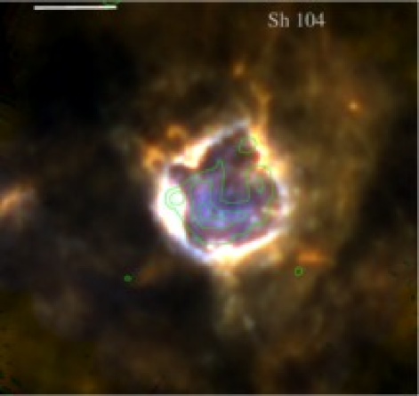
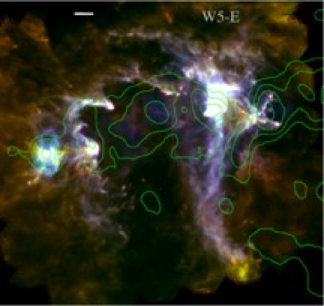
(a)

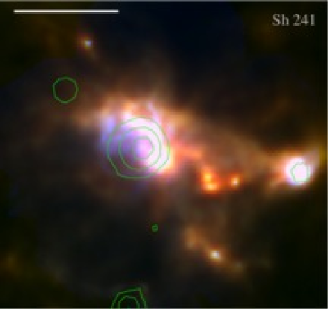
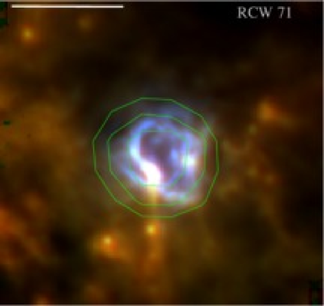
(b)

Figure 1: Three-color Herschel images for the eight observed regions. For each source the 500 $\,\mu{\rm m}$ data are shown in red, the 250 $\,\mu{\rm m}$ data in green, and the 100 $\,\mu{\rm m}$ data in blue. The images are oriented in RA and Dec. such that north is up and east is left. The white scale bar in the upper left corner is $5\arcmin$ in length. The coldest regions in each field appear red while the warmest appear blue. Contours show radio continuum emission from the NVSS (for Sh 104, Sh 241, and RCW 120), SUMSS (for RCW 79, RCW 82, and G332) or GB6 (for W5-E and RCW 71).

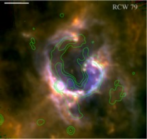
(c)

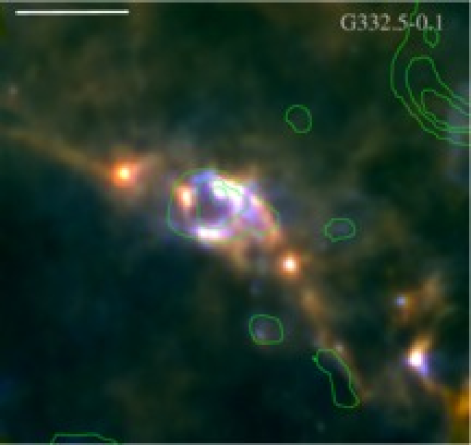
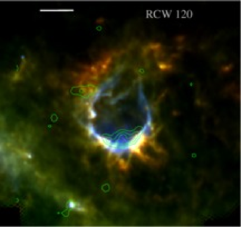
(d)

Figure 1: – continued.

2.1 Sh 104

Sh 104 (Sharpless, 1959) is a $\sim 7\arcmin$-diameter H II region. It has a shell of material located along the PDR that was detected in CO ($2\rightarrow 1$) observations by Deharveng et al. (2003). They estimate that the total mass in the shell is $\sim 6,\,000$ $\,M_{\odot}$. CS observations of the same field show four regularly-spaced dense molecular clumps on the border of Sh 104. One clump, of mass $\sim 670\,M_{\odot}$, is spatially coincident with an H II region detected in the NVSS. This region is seen on the eastern PDR of Sh 104 in Figure 1.

Russeil (2003) lists a kinematic distance for Sh 104 of $4.5^{+0.7}_{-0.8}$ kpc and a spectroscopic, or spectro-photometric, distance, of $3.1\pm 0.9$ kpc. Deharveng et al. (2003) used 4 kpc in their analysis, which we adopt for the present work. Sh 104 is excited by an O6V star (Crampton et al., 1978; Lahulla, 1985). Given the angular diameter, the physical diameter is $\sim\,8$ pc.

Sh 104 has strong 100 $\,\mu{\rm m}$ emission in its interior region (see 5.4). Also, it is the most “complete” of the H II regions in the sample in that the PDR is continuous and surrounds the entire region. These two phenomina may be related as the completeness of the PDR may indicate that radiation pressure and stellar winds are not particularly strong. In this scenario, the increased emission at 100 $\,\mu{\rm m}$ is a sign that the radiation is trapped in the bubble interior. There are numerous cold filaments that begin on the border of Sh 104 and lead radially away.

2.2 W5-E

W5-E (Westerhout, 1958) is a $\sim 34\arcmin$-diameter outer Galaxy H II region that has been the focus of numerous studies. It is part of the W3-W4-W5 complex; W4 and W3 are to the west of W5. Our observations are of W5-East, one part of the W5 region; the other part is W5-West, which is a second bubble that appears to be interacting with W5-East. Here we refer to “W5-East” as “W5-E.”

Here we adopt a distance of 2.0 kpc for W5-E. This distance is the same as the maser parallax distance assigned to W3(OH), $2.04\pm 0.07$ kpc (Hachisuka et al., 2006), and agrees well with estimates from spectroscopic parallax measurements (Becker & Fenkart, 1971; Moffat, 1972; Massey et al., 1995). The main exciting star of W5-E is HD 18326, which is of spectral type O7V (Walborn, 1973).

The Herschel image in Figure 1 shows a nearly complete bubble, open to the south. This southern opening is likely due to a density gradient in the ambient medium, as can be inferred from the CO observations in Heyer & Terebey (1998). There are also numerous “bright-rimmed clouds” (BRCs) and “elephant trunks” pointing toward the bubble interior. These features were seen in Spitzer observations of the region (Koenig et al., 2008), and are prime sites for investigating triggered star formation. Our observations contain three BRCs cataloged by Sugitani et al. (1991): BRC12, BRC13, and BRC14.

Point sources detected by Spitzer were analyzed by Koenig et al. (2008), who found two distinct populations of protostars; a population of Class II young stellar objects (YSOs) toward the interior of W5-E and a population of Class I YOSs in the surrounding molecular material. They hypothesize that these populations are separated by age and that triggering may have caused the creation of the Class I population.

A detailed study of star formation in W5-E using these same Herschel data is given in a companion paper, Deharveng et al. (2012).

2.3 Sh 241

Sh 241 (Sharpless, 1959) is a $\sim 3\arcmin$-diameter H II region. The region itself shows only faint H$\alpha$ emission (Pomarès et al., 2012, in prep.), although there is a dense adjacent molecular core that has been the focus of numerous studies in CS and HCN (Plume et al., 1992; Pirogov, 1999; Shirley et al., 2003; Wu et al., 2010). It has also been mapped at 350 $\,\mu{\rm m}$ (Mueller et al., 2002), a molecular outflow has been detected (Wu et al., 1999), and an H₂O maser has been detected (Cesaroni et al., 1988; Henning et al., 1992). Moffat et al. (1979) find that the spectroscopic distance to Sh 241 is $4.7$ kpc.

Sh 241 is the least complete of the bubble H II regions in our sample. Figure  1 shows that Sh 241 is open to the south and defined in the north by material that emits strongly in the FIR. There are numerous condensations in the field, especially to the west and south, and there is a separate H II region to the west detected in the NVSS. We note that there is faint emission seen to the south in Figure  1 that may be part of a secondary PDR of Sh 241. It is unclear if this is truly a secondary PDR however and the reported $3\arcmin$ size refers only to the more compact emission seen in at the center of the Herschel data.

2.4 RCW 71

RCW 71 (Rodgers et al., 1960) is a $\sim 3\arcmin$-diameter H II  region. Compared to the other H II regions in the sample, little is known about RCW 71. The Herschel images in Figure 1 show numerous small condensations to the south and west of RCW 71 that are bright at SPIRE wavelengths. The CO velocity of these condensations is similar to that of RCW 71 and are therefore likely associated (M. Pomarès, private communication). The PDR of RCW 71 seen in Figure 1 is filamentary. The spectroscopic distance of the exciting star of RCW71, HD311999, is 2.11 kpc while its near/far kinematic distances are 3.05/6.15 kpc (Russeil, 2003). The spectroscopic distance is in better agreement with distances to nearby young stellar clusters (Russeil et al., 1998) and we adopt the spectroscopic distance of 2.1 $\,{\rm kpc}$ for the present work. This gives a physical diameter for RCW 71 of $\sim 2$ pc.

2.5 RCW 79

RCW 79 (Rodgers et al., 1960) is a $\sim 12\arcmin$-diameter H II region. Using 1.2 mm continuum observations, Zavagno et al. (2006) found a fragmented layer of neutral material along the PDR of RCW 79 with a total mass of $\sim 2,\,000$ $\,M_{\odot}$. The mass of the most massive condensation is $\sim 1,\,000$ $\,M_{\odot}$. Zavagno et al. (2006) detected several Class I YSOs in the most massive condensations. The bright compact source seen to the south-east in Figure 1 is a separate H II region detected in radio continuum emission with SUMSS. Figure 1 shows that RCW 79 is open to the northwest. To the south, there is what appears to be a second ionization front.

Russeil (2003) find a kinematic distance of $4.8^{+0.9}_{-1.0}$ kpc for RCW 79 and a spectroscopic distance of $4.0\pm$0.6 kpc. We adopt 4 kpc for the present work, which leads to a physical diameter of 12 pc. Martins et al. (2010) found that RCW 79 is ionized by a cluster of a dozen O stars.

2.6 RCW 82

RCW 82 (Rodgers et al., 1960) is a $6\arcmin$-diameter H II region. Pomarès et al. (2009) studied the molecular emission traced with CO isolopologues surrounding RCW 82 and found a fragmented shell of emission with a total mass of $\sim 10,\,000$ $\,M_{\odot}$. The most massive condensations have masses of $\sim 2,500$ $\,M_{\odot}$. The YSO population identified by Pomarès et al. (2009) is not evenly distributed, but is concentrated on the border of RCW 82, indicating that triggered star formation may have lead to their formation.

RCW 82 appears along an IRDC filament detected on both sides of the H II region. The CO data in Pomarès et al. (2009) show that this filament is at the same velocity as RCW 82, and that the filament and H II region are therefore associated. There are numerous other filaments seen in Figure 1 that lead radially away from RCW 82; most are not seen in absorption at 8.0 $\,\mu{\rm m}$.

There is some uncertainty as to the distance to RCW 82. Russeil (2003) lists a kinematic distance of $4.3\pm 0.7$ kpc and a spectroscoptic distance of $2.9\pm 0.9$ kpc. Pomarès et al. (2009) use a distance of $3.4\pm 0.9$ kpc, which we adopt for the present work. Given the angular diameter and this assumed distance, the physical diameter of RCW 82 is 6 pc. Martins et al. (2010) find that RCW 82 is ionized by two O9–B2V/III stars.

2.7 G332.5$-$0.1

G332.5$-$0.1 is a $3\arcmin$-diameter H II region. It is located along a prominent IRDC running east-west, detected in emission at longer wavelengths with Herschel, that is associated with G332.5$-$0.1 in velocity (Deharveng et al., 2012b, in prep.). This filament, seen in Figure 1, has numerous sources within it detected by Herschel. G332.5$-$0.1 is unique in our sample in that hot dust at 100 $\,\mu{\rm m}$ is faint in its interior.

On the northern border of G332.5$-$0.1 there is an associated UC H II  region that has been the focus of numerous studies as part of the Red MSX Source survey (RMS; Urquhart et al., 2008). Just off the western border of G332.5$-$0.1 there is another region of extended radio continuum emission detected at 843 MHz with SUMSS and also at 24 $\,\mu{\rm m}$ with the MIPSGAL survey (Carey et al., 2009) – it is likely a distinct compact H II  region associated with G332.5$-$0.1.

The recombination line velocity of G332.5$-$0.1, $-50$ $\,{\rm km\,s^{-1}}$ from Caswell & Haynes (1987) places G332.5$-$0.1 at a kinematic distance of 3.7 $\,{\rm kpc}$. This assumes the near kinematic distance, which seems likely given its association with IRDCs (IRDCs at the far distance would be difficult to detect due to a lack of background behind the cloud). Russeil et al. (2005) have a slightly revised distance of 4.2 kpc for G332.5$-$0.1 based on nearby H II regions with a similar velocity; we use 4.2 kpc here which gives a physical diameter of $\sim 5$ pc.

2.8 RCW 120

RCW 120 (Rodgers et al., 1960) is an $8\arcmin$-diameter H II region that has been the focus of numerous recent studies. It has a massive, fragmented layer of neutral material seen along its PDR traced at mm (Zavagno et al., 2007) and sub-mm (Deharveng et al., 2009) wavelengths. Of the eight mm-condensations located by Zavagno et al. (2007), five are found on the PDR, indicating that this material has been collected during the expansion of the H II region. Deharveng et al. (2009) estimated that the mass of the collected layer is $\sim 2,\,000$$\,M_{\odot}$.

RCW 120 is among the nearest H II regions to the Sun. Russeil (2003) lists a kinematic distance of $1.8^{+0.6}_{-0.7}$ kpc and a stellar distance of $1.3\pm 0.4$ kpc for RCW 120; we adopt 1.3 kpc for the present work. Given the angular size, the physical size of RCW 120 is $\sim 3$ pc. A single star is ionizing RCW 120: CD$-38\,^{\circ}11636$. Georgelin & Georgelin (1970) found that its spectral type is O8 from spectroscopic measurements while (Crampton, 1971) find that it is an O9. More recently, using near-IR integral field spectroscopy, Martins et al. (2010) found that RCW 120 is ionized by a O6-8V/III star.

There is significant active star formation in the surroundings of RCW 120. Zavagno et al. (2007), Deharveng et al. (2009), and Zavagno et al. (2010) all located YSOs in the field. The most massive condensation is known as “Condensation 1” and is located to the south-west in Figure 1. Within Condensation 1, Deharveng et al. (2009) found an evenly spaced chain of eleven Class I or flat spectrum sources parallel to the IF. The authors suggest that it is an example of the Jeans gravitational instability. Using the same Herschel data shown here, Zavagno et al. (2010) detected a massive YSO towards Condensation 1 with a stellar mass of 8–10$\,M_{\odot}$. This condensation was detected previously at 70 $\,\mu{\rm m}$ by Spitzer (Deharveng et al., 2009). Zavagno et al. (2010) suggest that this is the first detection of a massive Class 0 object formed by the collect and collapse process on the border of an H II region.

There are also numerous IRDCs seen in the periphery of RCW 120, many with point sources observed in the mid-infrared suggestive of active star formation. The largest IRDC, G348.40+00.47, is observed to the north-east of RCW 120 in Figure 1. Jackson et al. (2008) measure a CS velocity of $-6.8$ $\,{\rm km\,s^{-1}}$   for G348.40+00.47, which is close to the recombination line velocity of the ionized gas in RCW 120, $-12$ $\,{\rm km\,s^{-1}}$ (Caswell & Haynes, 1987). The IRDC and the H II  region are therefore likely associated. We assume the smaller IRDCs to the north and west are also at the same distance as RCW 120. There are numerous cold filaments to the south of RCW 120 observed by Herschel, some of which are also seen in absorption at 8.0 $\,\mu{\rm m}$.

3 Observations and Data

In addition to the Herschel data that is the main focus of this work, we utilize auxilliary data from Herschel Hi-Gal, Spitzer GLIMPSE, Spitzer MIPSGAL, and APEX-LABOCA ATLASGAL. These auxillary data are available for four of our objects: RCW 79, RCW 82, G332.5$-$0.1, and RCW 120.

There are numerous point sources detected at all wavelengths for the H II regions in our sample. We make no attempt to remove them from the data. This is primarily because we cannot with confidence separate the sources from the local background at all wavelengths, while ensuring that we are locating the same source at all wavelengths. For example, an embedded source in a small IRDC can easily be identified at MIR wavelengths, but at the longest Herschel wavelengths with lower angular resolution, its emission extends over the entirety of the IRDC. If we were to remove this source, we would likely be removing a large fraction of the flux from the IRDC as well, preferentially for data with lower angular resolution.

3.1 Herschel HOBYS and “Evolution of Interstellar Dust”

Our sources were observed by the Herschel Space Observatory with the PACS (Poglitsch et al., 2010) and SPIRE (Griffin et al., 2010) instruments as part of the HOBYS (Motte et al., 2010) and “Evolution of Interstellar Dust” (Abergel et al., 2010) guaranteed time key programs. Data were taken in five wavelength bands from 100 $\,\mu{\rm m}$ to 500 $\,\mu{\rm m}$: 100 $\,\mu{\rm m}$ and 160 $\,\mu{\rm m}$ for PACS at FWHM resolutions of $6.7\arcsec$ and $11\arcsec$, and 250 $\,\mu{\rm m}$, 350 $\,\mu{\rm m}$, and 500 $\,\mu{\rm m}$ for SPIRE at FWHM resolutions of $18\arcsec$, $25\arcsec$, and $37\arcsec$. For both instruments, the observations were composed of two orthogonal scans. For all observations with the PACS instrument, the scan-speed was $20\arcsec$ per second while for SPIRE it was $30\arcsec$ per second. The observational parameters are summarized in Table 2, which lists for each source the field size, the total integration time, the observation identification numbers, and the observation date for observations with the PACS and SPIRE instruments. These data are available from the Herschel Science Archive.

Calibration for the 100 $\,\mu{\rm m}$ and 160 $\,\mu{\rm m}$ PACS bands using five standard stars has been found to be good to within $\sim 3\%$ at 100 $\,\mu{\rm m}$ and $5\%$ at 160 $\,\mu{\rm m}$ (see PACS Observers’ Manual). The extended source calibration is good to within $\sim 10\%$ at 70 $\,\mu{\rm m}$ and 100 $\,\mu{\rm m}$ and $\sim 20\%$ at 160 $\,\mu{\rm m}$; we adopt the latter numbers here. For SPIRE, the calibration is good to within 10% for all bands (see SPIRE Observers’ Manual). The SPIRE data are in Jy per beam and therefore we must know the beam size to convert to a flux density in Jy. Because of diffraction effects, the SPIRE beams are not entirely Gaussian – for flux calculations we use the modified beam areas of $423\arcsec^{2}$, $751\arcsec^{2}$, and $1587\arcsec^{2}$ for the 250 $\,\mu{\rm m}$, 350 $\,\mu{\rm m}$, and 500 $\,\mu{\rm m}$ bands (see Sibthorpe et al., 2011). The beam area at 250 is $\sim\,10\%$ larger than would be expected for a purely Gaussian beam while those at 350 $\,\mu{\rm m}$ and 500 $\,\mu{\rm m}$ are approximately that expected.

Table 2: Herschel observational parameters

	PACS				SPIRE
Name	Size	Time	ObsIDs	Date	Size	Time	ObsID	Date
	arcmin.	sec.		yyyy-mm-dd	arcmin.	sec.		yyyy-mm-dd
Sh 104	$20\times 20$	01730	1342185575, 1342185576	2010-10-10	$12\times 12$	0629	1342185535	2009-10-06
W5-E	$70\times 70$	13194	1342191006, 1342191007	2010-02-23	$65\times 60$	4309	1342192088	2010-03-11
Sh 241	$20\times 20$	01730	1342218725, 1342218726	2011-04-17	$15\times 15$	0770	1342192093	2010-03-11
RCW 71	$\phantom{0}9\times 9\phantom{0}$	00402	1342189389, 1342189388	2010-01-16	$\phantom{0}6\times 6\phantom{0}$	0332	1342203561	2010-08-23
RCW 79	$30\times 30$	02768	1342188880, 1342188881	2010-01-03	$19\times 19$	0837	1342192054	2010-03-10
RCW 82	$20\times 20$	01354	1342188882, 1342188883	2010-01-03	$12\times 12$	0571	1342192053	2010-03-10
G332.5$-$0.1	$22\times 22$	00817	1342204085, 1342204086	2010-09-05	$10\times 10$	0546	1342192055	2010-03-10
RCW 120	$30\times 30$	03302	1342185553, 1342185554	2009-10-09	$22\times 22$	1219	1342183678	2009-09-12

We reduce all Herschel data using slightly modified versions of the default PACS and SPIRE pipelines within the Herschel Interactive Processing Environment (HIPE) software, version 7.1. The level 2 pipeline-reduced data products from both instruments suffer from striping artifacts in the in-scan directions. Additionally, the level 2 PACS data have artifacts (flux decrements) around bright zones of emission caused by the median filtering baseline removal. To limit both the striping and the artifacts, we use the Scanamorphos software (Roussel, 2012), version 9. Scanamorphos estimates the true measured value at each sky position by exploiting the redundancy in the data. We use Scanamorphos without the “Galactic” option; in this configuration, the large-scale gradients of the sky emission are removed. During a typical Herschel observation, each sky position is observed by multiple bolometers in multiple scans. These multiple observations of the same sky positions can be used to estimate the true sky level. We have found Scanamorphos to be very effective at limiting striping without the addition of artifacts around bright emission zones. Scanamorphos also estimates the photometric uncertainty at each sky position using the weighted variance of all the samples contributing to each pixel. These uncertainty maps are useful because at present there is no propagation of the errors associated with each processing step in HIPE. We use these uncertainty maps in the aperture photometry described in §4.

The astrometry of the PACS and SPIRE Herschel data show offsets relative to each other, but also relative to higher-resolution Spitzer data. We found that the two PACS bands are well-aligned with respect to each other, as are the three SPIRE bands. To mitigate the astrometry effects, we align the PACS 100 $\,\mu{\rm m}$ data to the MIPSGAL data using point sources detected at both 100 $\,\mu{\rm m}$ and 24 $\,\mu{\rm m}$ in the Spitzer MIPSGAL survey (see below). We use the same astrometry solution for the PACS 160 $\,\mu{\rm m}$ data. Using point sources detected at 250 $\,\mu{\rm m}$ and 160 $\,\mu{\rm m}$, we then align the SPIRE 250 $\,\mu{\rm m}$ data to the PACS 160 $\,\mu{\rm m}$ data and accept the same solution for the SPIRE 350 $\,\mu{\rm m}$ and SPIRE 500 $\,\mu{\rm m}$ data. Offsets were $<10\arcsec$ for all regions, in all PACS and SPIRE bands.

The Herschel data for RCW 120 and Sh 104 were first shown in Anderson et al. (2010) and Rodón et al. (2010), respectively. The data presented in these articles were processed with slightly modified versions of the default PACS and SPIRE pipelines within HIPE version 2.0. Some of our results differ from those of Anderson et al. (2010) and Rodón et al. (2010), in part as a result of this new processing (see Section 5.2).

The new data processing differs from the old processing in that: 1) baselines (i.e. drifts on timescales larger than the scan leg crossing time) are now estimated by Scanamorphos using the redundancy in the data instead of a high-pass filter; 2) small-timescale drifts are also derived from the redundancy in Scanamorphos (they were either neglected [for SPIRE], or attenuated by Fourier filtering [for PACS] within HIPE); 3) data projection is done using a projection matrix in Scanamorphos for SPIRE data, which prevents biases between beam center and the projection center (HIPE used a nearest-neighbor projection); and 4) Scanamorphos includes relative gain corrections for SPIRE, taking into account beam variations from bolometer to bolometer, and reducing errors in maps of extended emission; 5) the newer version of HIPE used here has updated calibration values.

3.2 Herschel Hi-Gal

The Hi-Gal survey (Molinari et al., 2010), when complete, will map the entire Galactic plane using the PACS and SPIRE detectors of Herschel. While the Hi-Gal data are less sensitive than the observations shown here, Hi-Gal uses the PACS detector to observe at 70 $\,\mu{\rm m}$, a band not utilized with our observation mode. Here we use the Hi-Gal 70 $\,\mu{\rm m}$ data for RCW 79, RCW 82, G332.5$-$0.1, and RCW 120, the four regions that overlap with the current Hi-Gal coverage. These data have a spatial FWHM resolution of $6\arcsec$.

3.3 Spitzer GLIMPSE

We also use 8.0 $\,\mu{\rm m}$ data from the Spitzer Galactic Legacy Infrared Mid-Plane Survey Extraordinaire (GLIMPSE; Benjamin et al., 2003). GLIMPSE extends from $+60\degr\geq l\geq-60\degr$, $|b|\leq 1\degr$. The 8.0 $\,\mu{\rm m}$ IRAC (Fazio et al., 2004) filter contains, in addition to the continuum emission of hot dust, polycyclic aromatic hydrocarbon (PAH) bands at 7.7 $\,\mu{\rm m}$ and 8.6 $\,\mu{\rm m}$. These molecules emit strongly when excited by far-UV photons and thus can be used to trace ionization fronts. The same 8.0 $\,\mu{\rm m}$ IRAC band also shows many absorption features, IRDCs, which have been shown to be dense molecular clouds (e.g. Simon et al., 2006; Pillai et al., 2006). The resolution of the GLIMPSE 8.0 $\,\mu{\rm m}$ data is $\sim 2\arcsec$.

3.4 Spitzer MIPSGAL

The Spitzer MIPSGAL survey (Carey et al., 2009) at 24 $\,\mu{\rm m}$ and 70 $\,\mu{\rm m}$ mapped the Galactic plane from $+60\degr\leq l\leq-60\degr$, $|b|\leq 1.0\degr$ with the MIPS instrument (Rieke et al., 2004). Here we use only data at 24 $\,\mu{\rm m}$. At 24 $\,\mu{\rm m}$, the emission from H II regions has two components. First, there is emission from very small grains (VSGs) out of thermal equilibrium. This emission is detected in the interior area of the H II region (see Watson et al., 2008; Deharveng et al., 2010). Secondly, there is thermal emission from the PDR from grains that appear to be in thermal equilibrium. These two components have roughly equal fluxes for Galactic bubbles (Deharveng et al., 2010, §5.4). The resolution of the 24 $\,\mu{\rm m}$ MIPSGAL data is $\sim 6\arcsec$.

3.5 APEX-LABOCA ATLASGAL

Finally, we use data from the APEX Telescope Large Area Survey of the Galaxy at 870 $\mu$m (ATLASGAL; Schuller et al., 2009). ATLASGAL extends from $+60\degr\geq l\geq-60\degr$, $|b|\leq 1.5\degr$ and has a spatial FWHM resolution of $19\arcsec$. The ATLASGAL survey was performed with the Large Apex BOlometer CAmera (LABOCA), a 295-pixel bolometer array (Siringo et al., 2009). For RCW 120, instead of ATLASGAL, we use more sensitive pointed APEX-LABOCA observations first shown in Deharveng et al. (2009). In the processing of APEX-LABOCA data, large-scale low amplitude structures $>2.5\arcmin$ are filtered out. The calibration uncertainty in ATLASGAL is $\,\lesssim\,15\%$ (Schuller et al., 2009).

4 The Dust Properties of Galactic Bubbles

Assuming optically thin emission, the flux from a population of dust grains can be modeled as a modified blackbody:

$$F_{\nu}\propto\kappa_{\nu}\,B_{\nu}(T_{d})\,N_{\rm dust}\,,$$ (2)

where $F_{\nu}$ is the flux density per beam, $\kappa_{\nu}$ is the dust opacity in cm² g^-1, $B_{\nu}(T_{d})$ is the Planck function for dust temperature $T_{d}$ at frequency $\nu$ (here in Jy sr^-1), and $N_{\rm dust}$ is the dust column density in cm^-2. The dust opacity law we assume for the present work is given in Equation 1. To derive the total hydrogen column density and mass (gas+dust), we must assume a gas to dust ratio, $R$. The column density of gas and dust is:

$$N_{\rm H}=R\,\frac{F_{\nu}}{2.8\,m_{\rm H}\,\kappa_{\nu}\,B_{\nu}(T_{d})\,\Omega}\,,$$ (3)

where $m_{\rm H}$ is the mass of a hydrogen atom in g, the factor of 2.8 accounts for elements heavier than hydrogen, and $\Omega$ is the beam size in steradians. The total mass of dust and gas in g may then be estimated from the integrated flux in Jy, $S_{\nu}$ (cf. Hildebrand, 1983):

$$M=R\,\frac{S_{\nu}\,D^{2}}{{\kappa_{\nu}}\,B_{\nu}(T_{d})}\,,$$ (4)

where $D$ is the distance in cm. The preceeding equations assume that the measured flux at frequency $\nu$ is entirely due to thermal dust emission. For the present work, at 350 $\,\mu{\rm m}$, we assume the functional form for the dust opacity given in Beckwith et al. (1990), $\kappa_{\nu}\leavevmode\nobreak\ =\leavevmode\nobreak\ 10(\nu)^{\beta}$, where $\nu$ is in THz and we assume $\beta=2$. This leads to an opacity at 350 $\,\mu{\rm m}$ of $\kappa_{350}\leavevmode\nobreak\ =\leavevmode\nobreak\ 7.3$ cm² g^-1, which we use throughout. For all mass calculations, we assume that the dust-to-gas mass ratio has a value of 100. These values for $\kappa_{\nu}$ and $R$ are uncertain, which leads to large uncertainties in the mass and column density estimates. For example, Preibisch et al. (1993) estimate that using the above formulation to compute masses results in uncertainties of up to a factor of five. Errors in distances for some sources may be up to a factor of two in extreme cases, further increasing the uncertainty of the mass estimates.

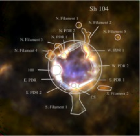
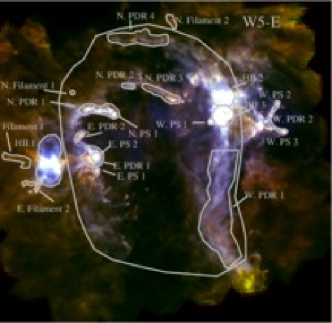
(a)

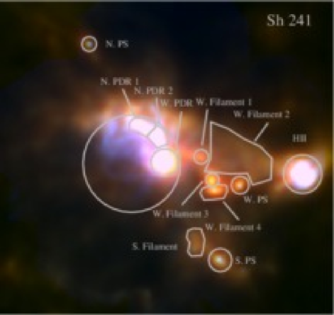
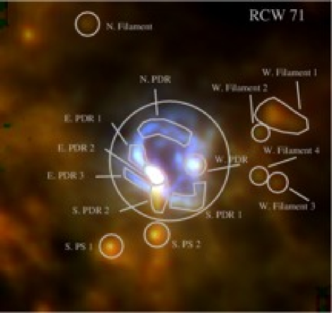
(b)

Figure 2: Same as Figure 1, but showing the regions used in the aperture photometry. As in Figure 1, the three-color images are composed of Herschel data for each source with 500 $\,\mu{\rm m}$ in red, 250 $\,\mu{\rm m}$ in green and 100 $\,\mu{\rm m}$ in blue. The apertures used for the aperture photometry measurements are shown in gray outline.

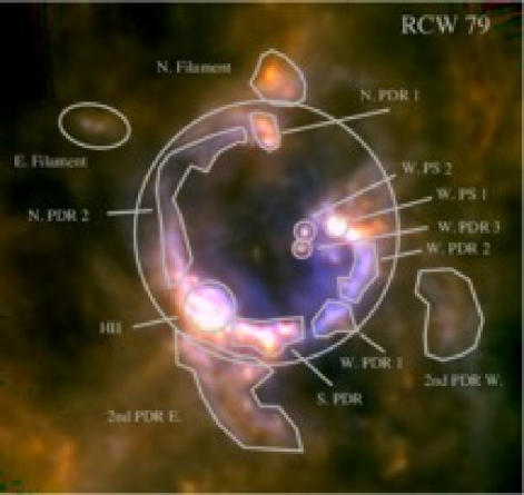
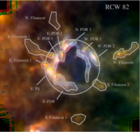
(c)

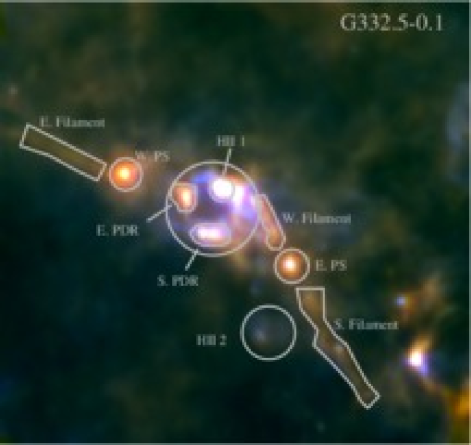
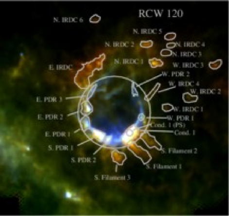
(d)

Figure 2: – continued.

4.1 Aperture Photometry

Aperture photometry allows us to derive the average dust properties within an aperture of arbitrary size and shape. The measured flux within an aperture contains the combined emission along the line of sight. Most of the regions studied here are optically visible and thus the extinction along the line of sight is relatively low. The contribution to the fluxes from dust along the line of sight not associated with the H II region is therefore minimized, but cannot be completely absent.

We define the apertures by eye to include contiguous regions of dust emission from a volume that can be characterized by a single temperature value. This process is subjective; we use the three-color images shown in Figure 1 to help define regions where the temperature variation within the region is not severe. In addition to specific regions of interest, we define for each H II region a large aperture that includes all emission associated with the H II region itself, but not the emission associated with local clouds or filaments. The apertures are shown in Figure 2 on top of the same Herschel data shown in Figure 1. In total, we define 129 apertures.

We visually categorize the apertures into five classifications based on their location and appearance in the Herschel data. The five aperture classes are: “Entire” for the largest apertures that include all the emission from the H II region (including that of hte PDR), “Other H II” for the apertures that include emission from other H II regions in the fields, “PDR” for locations along the PDRs, “Point source” for apertures containing only the emission from sources that appear point-like at 100 $\,\mu{\rm m}$ (including possibly their outer envelope detected at longer wavelengths), and “Filament” for apertures that enclose extended structures detected at 250 $\,\mu{\rm m}$ that are not along PDRs and that are not the longer-wavelength emission of point-like objects detected at 100 $\,\mu{\rm m}$. Because filaments seen in absorption at 8.0 $\,\mu{\rm m}$ must be dense and therefore may be especially cold, we subdivide the “Filament” class into those seen in absorption at 8.0 $\,\mu{\rm m}$ (IRDCs), and those that are not seen in absorption at 8.0 $\,\mu{\rm m}$. Excluding the “Entire” and “Other H II ’́ classes, which both contain eight apertures, there are 113 apertures. Of these, 49 are classified as “PDR”, 46 as “Filament” (with 17 as infrared dark filaments), and 18 as “Point source”.

Many of the apertures for RCW 120 and Sh-104 were defined previously in Anderson et al. (2010) and Rodón et al. (2010), respectively. We have made some modifications to the apertures shown in these works: we have changed the shape of some apertures, added new apertures to highlight additional regions of interest, removed apertures that either cannot be well-characterized by a single dust temperature, and given some apertures a different name. The new aperture shapes should better contain dust that can be characterized by a single temperature, and are more consistant between all regions in the current sample. We removed apertures in the direction of the “interior” of the bubbles because of the difficulty of fitting a single dust temperature. The aperture names used here better reflect the location of the aperture and again are more consistant with the naming convention employed for the other regions in our sample.

In addition to the “bubble” H II regions that we targeted in our observations, there are eight additional sources in the Herschel fields that have characteristics of H II regions. All of these eight sources have spatially coincident IR (from Herschel and Spitzer) and radio emission from the NVSS or SUMSS. Together spatially coincident IR and radio emission point to a thermal source (Haslam & Osborne, 1987; Broadbent et al., 1989; Anderson et al., 2011), e.g., a planetary nebula (PN) or an H II region.

Anderson et al. (2012) derive IR color criteria for distinguishing between PNe and H II regions. To determine the classification of the eight other H II regions, in addition to the aperture photometry described below we compute aperture photometry using the Wide-field Infrared Survey Explorer (WISE) data at 12 $\,\mu{\rm m}$ and 22 $\,\mu{\rm m}$. All the H II regions tested satisfy the criterion found by Anderson et al. (2012): ${\rm log(}F_{160}/F_{12})>1.3$, where $F_{160}$ is the flux at 160 $\,\mu{\rm m}$ from Herschel and $F_{12}$ is the flux at 12 $\,\mu{\rm m}$ from WISE and in fact all have ${\rm log(}F_{160}/F_{12})>2$. Anderson et al. (2012) found that 10% of their sample of PNe satisfy ${\rm log(}F_{160}/F_{12})>1.3$ and no PNe satisfy ${\rm log(}F_{160}/F_{12})>2$. Together with the spatially coincident IR and radio emission, these criteria suggest that these sources are bona fide H II regions. There are no WISE data available for the additional H II region located on the PDR of Sh2-104. Since this source satisfies the criteria for UC H II regions in Wood & Churchwell (1989a) and has detected CS emission (Bronfman et al., 1996), it is almost surely an H II region and not a PN. We assume throughout following that the eight other H II regions are at the same distance as the bubble H II regions that were targeted. This assumption may not hold for H II regions well-separated in angle from the bubble H II regions, i.e., for one of the H II regions in the field of G332 and the second H II region in the field of Sh 241.

Because our data have a range of resolutions, we smooth all data to the lowest resolution SPIRE 500 $\,\mu{\rm m}$ data, which has a resolution of 37 ″. To mediate pixel edge effects, we rebin all data sets so they have the same pixel size and location using the Montage software.

For each H II region, we compute the flux at all available wavelengths for each aperture. In this process we utilize the Kang software, version 1.3, which contains routines to perform aperture photometry with apertures of arbitrary size and shape, and accounts for fractional pixels. We estimate the errors at each wavelength by summing in quadrature the calibration uncertainties given in §3 and the photometric error as calculated by Scanamorphos. For Herschel data, we compute the photometric error by adding in quadrature the individual errors of all pixels within the aperture from the error maps produced by Scanamorphos. For the other data sets, we estimate the photometric error using the standard deviation of the background region multiplied by the square root of the number of pixels in the aperture.

We subtract from each aperture flux, at each wavelength, a background value. For apertures at the center of the frame (mainly the “Entire”, “Other H II,” and “PDR” classes) we use a single background value at each wavelength for all apertures. Because apertures in these classifications generally have high fluxes, we have found that the exact choice of background value does not severely impact our results. A single background value, however, does not approximate the true background level accross the entire field. Therefore, for apertures located away from the center of the frame we define a local background value. The removal of a background is necessary because the true “zero-point” for our observations is unknown. Perhaps more importantly, however, there are potentially contributions from multiple emission regions along the line of sight. In the Scanamorphos data reduction, we remove the general gradients of the sky emission within the field of view (by not using the “Galactic” option) and therefore we believe the flat background approximation is valid; attempts to remove a more complicated background were met with difficulty due to the relatively small size of our fields.

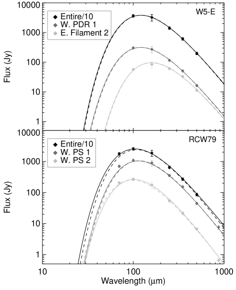
Figure 3: Example SEDs fits for regions within W5-E (top) and RCW 79 (bottom). The solid curves show the $\beta=2.0$ trial and the dashed curves show the $\beta$-free trial. We do not have 70 $\,\mu{\rm m}$ or 870 $\,\mu{\rm m}$ data for W5-E, and we exclude the 870 $\,\mu{\rm m}$ point from the fit to the “Entire” aperture for RCW 79.

We construct a spectral energy distribution for each aperture using the background-corrected fluxes at wavelengths from 70 $\,\mu{\rm m}$ to 870 $\,\mu{\rm m}$. Using the “MPFIT” least-squares minimization routines in IDL (Markwardt, 2009), we then fit Equation 2 in two trials: once with the normalization and dust temperature as free parameters and $\beta$ fixed to a value of 2.0 and once with the normalization, dust temperature, and $\beta$ as free parameters. In the SED fits, we generally include data at both 70 $\,\mu{\rm m}$ and 100 $\,\mu{\rm m}$, although there is likely some contribution from a warmer dust component at these wavelengths. We do, however, exclude data at 70 $\,\mu{\rm m}$ from IRDC apertures because at this wavelength they may be optically thick and we exclude 870 $\,\mu{\rm m}$ data from the “Entire” apertures because these data are not sensitive to large-scale diffuse emission. Emission from warmer dust is detected mainly toward the interior of the bubbles in our sample – it has minimal impact on the parameters derived here (see §5.4). Using Equation 4, we also calculate the mass within each aperture.

The measured flux within a photometric bandpass is a function of the shape of the SED across the bandpass and of the shape of the bandpass itself. Each measured flux is therefore a function of temperature and $\beta$. To correct for this issue, we perform a “color correction” on the measured fluxes. During the spectral fitting, we iteratively apply color correction factors by repeatedly fitting a temperature and $\beta$ then applying the corresponding correction factors until successive fit results are unchanged. For SPIRE, these color correction factors, given in the SPIRE Observers’ Manual, are $<10\%$ for all values of $\beta$ considered here. For PACS, the color correction factors are given in Poglitsch et al. (2010). The PACS color correction factors can be quite large at low temperatures, especially for the 70 $\,\mu{\rm m}$ band. For example, at 10 K, the correction factor is 3.65 for the 70 $\,\mu{\rm m}$ band and 1.71 for the 100 $\,\mu{\rm m}$ band. At 15 K, the respective factors are 1.61 and 1.16. While these correction factors are large, we find that the net impact on the derived temperature is small. For the apertures used here, the mean absolute temperature difference between apertures fit without a color correction and the same apertures fit with a color correction is 0.6 K, or $\sim 3\%$.

The results of the aperture photometry analysis are given in Table 3. This table lists for each aperture the name shown in Figure 2, mean Galactic longitude and latitude, the angular size of the aperture in square arcminutes, the derived dust temperature and mass for the two fit trials, the $\beta$-values for the $\beta$-free trial, and the classification. The errors in dust temperature and $\beta$ account for calibration uncertainty and photometric errors. We show in §5.2 that they are good estimates of the errors in the derived quantities. Example fits are shown in Figure 3 for three apertures within W5-E and RCW 79.

4.2 Maps of Dust Properties

The high-angular resolution Herschel data also allow us to produce two-dimensional maps showing the distributions of temperature and column-density. With such maps, we may examine both small- and large-scale variations in dust properties. These maps have the resolution of the 500 $\,\mu{\rm m}$ data, $37\arcsec$ and are available from the authors upon request.

4.2.1 Temperature Maps

We construct temperature maps for each of the eight regions in our sample by fitting the SED extracted at a grid of locations using Equation 2. When doing so, we use the same chi-squared minimization routine used for the aperture photometry and again leave the column density as a free parameter. In the creation of the temperature maps, we again include data at 70 $\,\mu{\rm m}$; including the 70 $\,\mu{\rm m}$ emission differs from the method of other authors (e.g., Hill et al., 2011). The effect of including data at this wavelength is explored in §5.4.

While the wavelength coverage of Herschel and the number of data points is theoretically sufficient to simultaneously fit for $T_{d}$ and $\beta$, we find that the uncertainties in such fits are large and the correlation between the derived temperatures and the values derived in the aperture photometry is weak. We therefore hold $\beta$ fixed to a value of 2.0 when creating the maps, which is the average value found in the aperture photometry.

We remove a flat average background level from the smoothed, rebinned data at each wavelength. The background value was defined such that 99.99% of the pixels in the resultant images have an intensity greater than zero. This ensures that nearly all locations have positive flux values. This method of background subtraction is different from the method of the aperture photometry but is necessary to ensure that background-subtracted pixels have a positive intensity value, and thus that we will be able to determine the dust temperature and column density over the entire map.

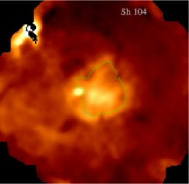
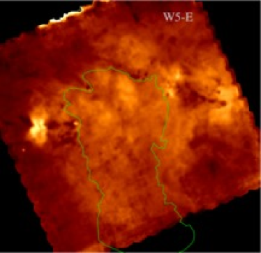
(a)

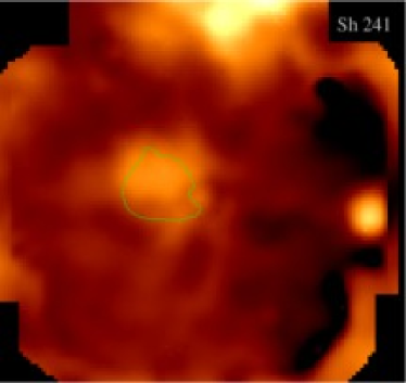
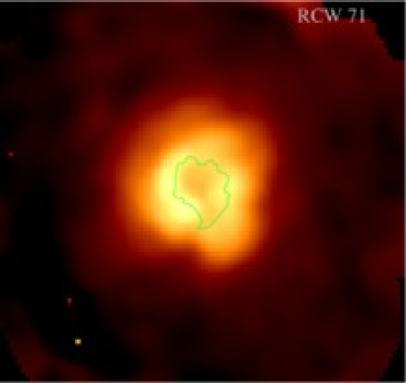
(b)

Figure 4: Temperature maps created by fitting the SEDs extracted at a grid of locations. All panels have the same color scale and range from 15 K to 35 K. The green curves show the approximate extent of the bubble interiors.

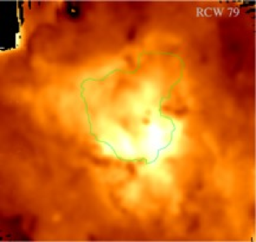
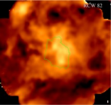
(c)

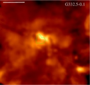
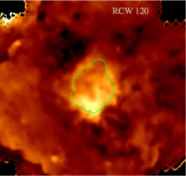
(d)

Figure 4: – continued.

We show temperature maps for the eight regions in Figure 4 for the same map areas shown in Figures 1 and 2. The highest temperatures, $\sim 40$ K, are found in the direction of the interior regions of the bubbles and toward other local H II regions. The coldest temperatures, $\sim 12$ K, are found for the IRDCs and other regions designated as “filaments” in the aperture photometry (§4.1). Errors in the derived temperatures for individual pixels are generally less than 10%. Large patches of very high temperatures on the periphery are in general not real, but are caused by low emission (e.g., to the north-east of Sh 104, to the north of Sh 241, and to the north-east of RCW 82).

Figure 4 shows a wide range of temperature structures. For Sh 104, Sh 241, RCW 79, RCW 120, and RCW 82, the bubble interiors show increased temperatures. These temperatures are quite uncertain though and individual SEDs often show contributions from multiple components (see §5.4). The hottest temperatures for RCW 71, however, are in the PDR. For G332.5$-$0.1 the hottest dust temperature is also along the PDR, to the north, coincident with the UC and compact H II regions. W5-E shows little variation in temperature although there are warmer locations associated with the other H II regions in the field. Variations within the fields of individual regions are dicussed in Appendix LABEL:sec:individual.

The temperature map values agree with the results of the aperture photometry, but there are large differences for colder regions. To compare the two methods of deriving tempatures, we compute the average dust temperature found in the temperature map within the apertures used previously. In Figure 5, we plot the temperature derived in the aperture photometry versus the average temperature map temperature for each aperture. We find that the two temperatures are on average 12% different, or roughly 2.3 K. This difference is pronounced for apertures with temperatures less than 15 K and warmer than 30 K, for which the temperature map values are sytematically higher or lower, respectively. These discrepancies are due to the differences in background treatment between the two methods. Because we evaluate the background individually for each aperture, we believe the aperture photometry dust temperature values are more accurate. The circled points in Figure 5 are IRDCs in the field of RCW 120; they account for much of the difference at low temperature. The difference in temperature for these cold regions is due to our assumption of a flat background in the temperature maps. For cold regions this assumption causes us to overestimate the temperature, while the inverse is true for warm regions. We do not expect a perfect correlation because the aperture photometry temperatures are weighted toward the highest emitting regions within the aperture. The mean standard deviation of temperature map values within the apertures is 2.0 K.

4.2.2 Column Density Maps

From the temperature maps, we also create column density maps using Equation 3. As mentioned above, we evaluate $\kappa_{\nu}$ at 350 $\,\mu{\rm m}$, and assume a value of $\kappa_{350}$ = 7.3 cm² g^-1 and a dust-to-gas mass ratio of 100. At each grid location in the column density map, we calculate the Planck function value $B_{\nu}(T_{d})$ using the derived temperature from the temperature map. For the flux at 350 $\,\mu{\rm m}$, we use the Herschel SPIRE image data, after removing a background value defined as before such that 99.99% of the pixels at 350 $\,\mu{\rm m}$ have an intensity greater than zero. The removal of a background value produces a more realistic picture of the column density associated with each region, rather than the total integrated column density along the line of sight. The resultant maps are shown in Figure 6.

The column density distributions in Figure 6 shows enhancements along the bubble PDRs. These enhancements likely are from the material swept up during the expansion of the H II region. For RCW 71, however, the PDR is barely enhanced relative to the background. Other prominent column density enhancements in the fields are generally caused by filaments, especially IRDCs, and unresolved sources. For comparison, the IRDCs in Peretto & Fuller (2010) have typical column densities of $\gtrsim 10^{22}\,{\rm cm^{-2}}$. The highest column densities are generally associated with condensations with detected protostars inside (i.e. Condensation 1 in RCW 120). Column density values toward the bubble interiors are uncertain due to uncertainties in temperature and because of the low flux values found there. The spurious temperature values near the image edges mentioned previously result in spurious column density values as well (e.g., south-west of Sh 241 and south-east of RCW 71). A more complete discussion for individual regions is given in the Appendix.

PDRs and cold filaments share nearly the same mean column density values. We calculate the mean column density value shown in Figure 6 within the previously defined apertures for regions in the “PDR” and “Filament” classes. The average value for the “PDR” class is $1.8\times 10^{21}\,{\rm cm^{-2}}$ while it is $1.9\times 10^{21}\,{\rm cm^{-2}}$ for the “Filament” class. The above average values were calculated after first taking the log of the column density values, so large values of column density would not bias the result.

5 Discussion

5.1 Comparison of Aperture Classes

With the calculated values of $\beta$ and $T_{d}$ in Table 3, we may investigate how the dust properties change with location in the H II region environment using the aperture classifications. The easiest way to see differences in dust properties is in the shapes of the SEDs themselves. We show average SEDs for the classifications in Figure 7. To create Figure 7, we normalized the SED for each aperture by the highest flux and averaged all apertures for a given classification. The curves are therefore unweighted averages of the normalized fluxes. The “Entire,” “Other H II,” and “PDR,” classes have similar shapes, as do the “Filament” and “IRDC” classes. The “PS” class has a mean SED shape in between the two groupings. The similar shapes of the SEDs hint at similar dust properties for these classifications. Compared to the other classifications, the “Filament” and “IRDC” classes peak at longer wavelengths and show more emission in the FIR part of the SED. This shows that these apertures have colder mean temperatures.

Figure 5: The temperature derived using aperture photometry versus the average temperature in the temperature map derived using the same apertures. The line is not a fit but rather shows a 1:1 relationship. The circled sources are IRDCs from the field of RCW 120; they account for much of the difference at low temperature.

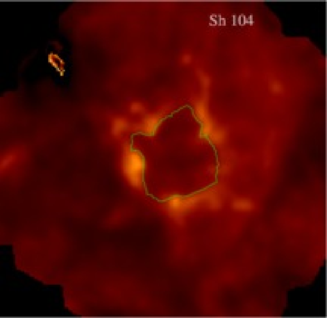
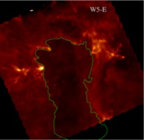
(a)

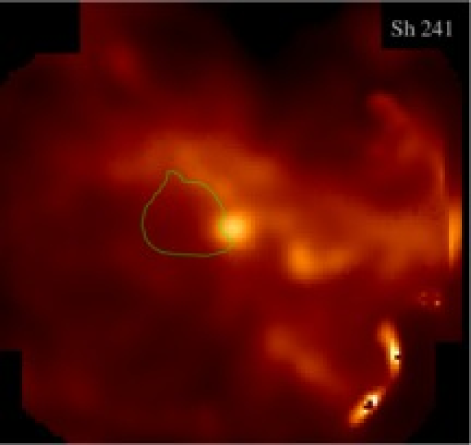
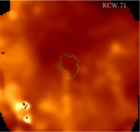
(b)

Figure 6: Column density maps created using Herschel 350 $\,\mu{\rm m}$ data and the temperatures shown in Figure 4. The scaling for all panels is the same; the values range from $10^{20}\,{\rm cm^{-2}}$ to $10^{22.5}\,{\rm cm^{-2}}$. The green curves show the approximate extent of the bubble interiors. Enhancements are seen along the bubble PDRs.

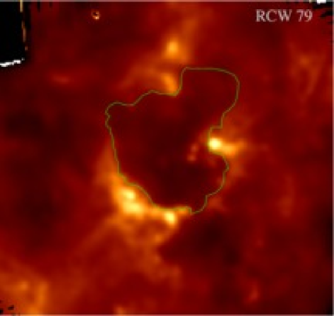
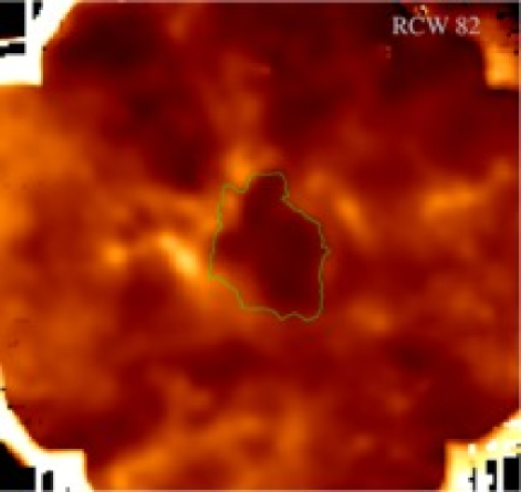
(c)

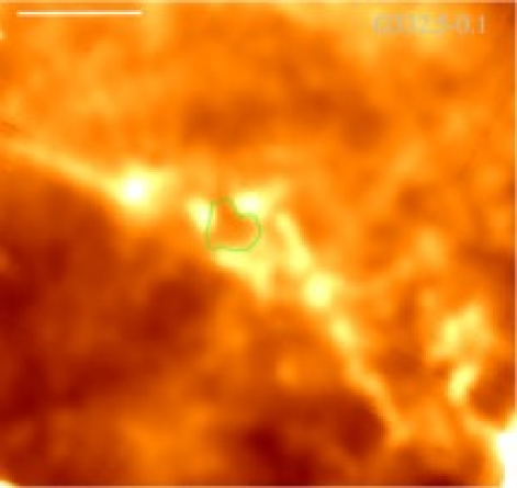
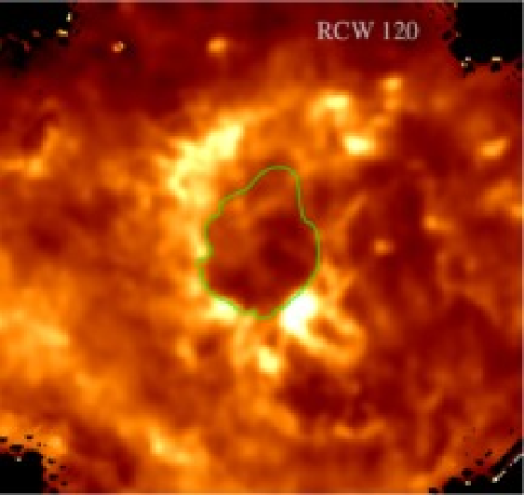
(d)

Figure 6: – continued.

We list the mean dust properties for each aperture classification in Table 4, which shows the average dust temperature and $\beta$-values for the $\beta=2$ trial and the $\beta$-free trial, together with their 1-$\sigma$ standard deviations, the percentage of apertures that have peak fluxes long-ward of 100 $\,\mu{\rm m}$, the percentage of apertures that have peak fluxes long-ward of 160 $\,\mu{\rm m}$, and the number of apertures of a given classification. The seventh and eigth columns dealing with the wavelength of the peak flux provide a check against the results of the temperature fitting – SEDs that peak long-ward of 160 $\,\mu{\rm m}$ have dust temperatures of $\lesssim\!12$ K while those that peak long-ward of 100 $\,\mu{\rm m}$ have dust temperatures of $\lesssim\!21$ K, assuming $\beta=2$. The row labeled “All Filaments” includes filaments of aperture classification “F” and infrared dark filaments of aperture classification “F (ID)” from Table 3. The rows labelled “IRDC” and “Not IRDC” contain only data from inner-Galaxy H II regions for which we have 8.0 $\,\mu{\rm m}$ data (RCW 79, RCW 82, G332.5$-$0.1, and RCW 120).

A difference in temperature has implications for subsequent star formation. The Jeans mass scales as $M_{J}\leavevmode\nobreak\ \propto\leavevmode\nobreak\ T^{3/2}\,\rho^{-1/2},$ where $\rho$ is the mass volume density, and therefore higher temperatures lead to higher values of $M_{J}$. The average temperature of the PDR classification, 25.6 K, is significantly higher than that of the filaments, 16.9 K. For the above average temperatures, if the gas and dust share the same temperature and the density in the PDR and the filaments is comparable, the Jeans mass would be $\sim 80$% higher in the H II region PDRs compared to the filaments. This would imply that on average higher mass stars will form in the H II region PDRs through gravitational collapse compared to the filaments. We stress, however, that the density is a large unknown here and further observations are needed to better constrain this parameter.

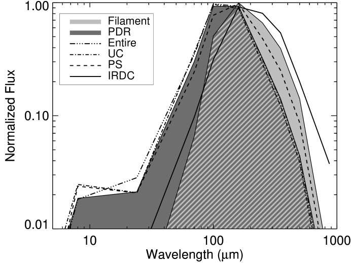
Figure 7: The average normalized SEDs for the aperture classes. Results from the “PDR” class are shown in dark gray while those in the “Filament” class are shown in light gray. Where the two “PDR” and “Filament” distributions overlap, we show light gray with dark gray hatching. Lines show the average normalized SEDs for the “Entire”, Other “HII,” “PS,” and “IRDC” classes; the “IRDC” class SED is similar to that of the “Filament” class while the SEDs of the “Entire”, and “Other H II” classes are more similar to that of the “PDR” class. The “PS” class has a mean SED shape in between that of the “PDR” and “Filament” classes. The points at 8.0 $\,\mu{\rm m}$ and 24 $\,\mu{\rm m}$ are shown here although these data were not used in the fits.

Table 3 and Figure 7 show that there are two broad classifications of apertures that can be grouped by their similar temperature values. The first is a “warm” group characterized by temperatures of $\sim 26$ K that includes the “Entire”, “Other H II”, and “PDR” aperture classifications. There is no statistical difference between all possible combinations of aperture classifications within the “warm” group, as shown by a Kolmogorov-Smirnov (K-S) test which assesses the probability that two distributions belong to the same parent distribution. The second “cold” group consists of apertures classified as “Filament” or “IRDC” and is characterized by dust temperatures of $\sim 17$ K. Some apertures in the “PS” classification have dust properties similar to those in the “warm” group, while some have dust properties more similar to those in the “cold” group; we do not include “PS” apertures in either group. This likely reflects the range of evolutionary states in this classification: the colder apertures of the “PS” class are in an earlier evolutionary state than the warmer ones that may be heated by a central young stellar object. In Figure 8, we show graphically how the “warm” and “cold” aperture groups, which were defined according to their aperture classifications and not according to their dust temperatures, have different temperature distributions. Roughly half of the apertures in the “warm” group have an emission peak long-ward of 100 $\,\mu{\rm m}$ while all the apertures in the “cold” group meet this criterion. There are no apertures in the “warm” group whose wavelength of peak flux emission is long-ward of 160 $\,\mu{\rm m}$, while 13% of the apertures in the “cold” group meet this criterion.

Filaments that are infrared dark at 8.0 $\,\mu{\rm m}$ are colder than those that are not infrared dark at 8.0 $\,\mu{\rm m}$. When $\beta$ is held fixed to 2.0, the “IRDC” filaments have a mean temperature of $15.5\pm 3.5$ K while the “Not IRDC” filaments have a mean temperature of $18.8\pm 2.9$ K; these values change to $14.7\pm 3.6$ K and $17.8\pm 2.2$ K respectively when $\beta$ is allowed to vary. A K-S test shows that the temperatures derived for the two groups when $\beta$ was held to 2.0 are significantly different. This suggests that IRDCs are colder versions of the filaments we identified. The detection of an IRDC relies on a strong IR background that the cloud can absorb against and some of the filaments not seen in absorption may simply be lacking sufficient background. Cold dust temperatures $T_{d}\leq 12$ K are also found in less massive filaments of nearby complexes (Bontemps et al., 2010; Arzoumanian et al., 2011) and thus such temperatures are not restricted to the more massive Galactic IRDCs.

Table 4: Dust properties by aperture classification

	$\beta=2$		$\beta$ free
Class.	$<\!T_{d}\!>$	$\sigma_{T_{d}}$	$<\!T_{d}\!>$	$\sigma_{T_{d}}$	$<\!\beta\!>$	$\sigma_{\beta}$	$>\!100\,\mu{\rm m}$	$>\!160\,\mu{\rm m}$	N
	K	K	K	K			%	%
${\rm Entire}$	$25.3$	$2.4$	$26.5$	$2.9$	$1.9$	$0.3$	$\phantom{0}50$	$\phantom{0}0$	$8$
${\rm Other\ HII}$	$26.1$	$2.0$	$26.2$	$3.2$	$2.0$	$0.3$	$\phantom{0}37$	$\phantom{0}0$	$8$
${\rm PS}$	$21.3$	$3.3$	$22.2$	$3.1$	$1.8$	$0.2$	$\phantom{0}83$	$\phantom{0}0$	$18$
${\rm PDR}$	$25.8$	$4.0$	$24.4$	$3.3$	$2.1$	$0.4$	$\phantom{0}61$	$\phantom{0}0$	$49$
${\rm All\ Filaments}$	$16.8$	$3.0$	$16.8$	$3.4$	$2.1$	$0.5$	$100$	$13$	$46$
${\rm\ \ \ \ IRDC}$	$15.5$	$3.5$	$14.7$	$3.6$	$2.2$	$0.4$	$100$	$29$	$17$
${\rm\ \ \ \ Not\ IRDC}$	$18.8$	$2.9$	$17.8$	$2.2$	$2.2$	$0.2$	$100$	$\phantom{0}0$	$8$

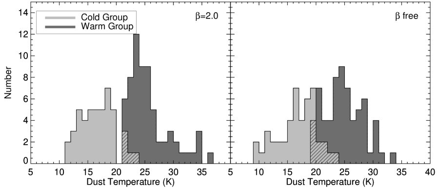
Figure 8: Dust temperatures of warm and cold aperture groups. Shown are the distributions for the apertures in the cold group (“Filament” and “IRDC” classifications) in light gray and the apertures in the warm group (“Entire,” “Other H II,” and “PDR” classifications) in dark gray. We do not include in this figure apertures with classification “PS”. Where the two distributions overlap, we show light gray with dark gray hatching. The left panel shows dust temperatures derived when $\beta$ was held fixed to a value of 2.0 while the right panel shows the dust temperatures derived when $\beta$ was allowed to vary. It is evident that these two aperture groups have different dust temperature distributions.

As shown in Table 4, apertures in the “warm” and “cold” groups share a similar distribution of $\beta$ values. We show these distributions graphically in Figure 9. Both groups are centered about $\beta=2.0$. The average error in $\beta$ is 0.3, which likely causes some of the spread in the distribution.

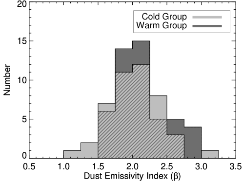
Figure 9: Dust opacity spectral index $\beta$ of warm and cold aperture groups. Shown are the distributions for the apertures in the cold group (“Filament” and “IRDC” classifications) in light gray and the apertures in the warm group (“Entire,” “Other H II,” and “PDR” classifications) in dark gray. Where the two distributions overlap, we show light gray with dark gray hatching. The two aperture groups have only slightly different dust emissivity index distributions. The typical error in $\beta$ for individual apertures is $\sim 0.3$.

5.2 The $\beta-T_{d}$ Relationship

As discussed in the Introduction, there is significant observational evidence for an anti-correlation between $\beta$ and dust temperature. It is therefore reasonable to expect the same correlation for our data. In Figure 10 we plot the dust temperature against $\beta$ for all apertures. We do not find a strong relationship between the two quantities. The data points in Figure 10 are coded such that apertures in the “warm” group are shown with filled circles and those in the “cold” group are shown with open circles. The “PS” apertures are shown with star symbols. The trend lines found by Dupac et al. (2003), Désert et al. (2008), Veneziani et al. (2010), and Paradis et al. (2010) are over-plotted, as is the best-fit line to our data. The trend lines found by previous others do not agree with our trend line. Most of these previous studies have used different wavelengths to those used here.

Using the same functional form as Désert et al. (2008), our best-fit line follows the relationship:

$$\beta=(4.3\pm 0.5)\,T_{d}^{-0.2\pm 0.04}\,.$$ (5)

A linear fit follows the relationship:

$$\beta=2.6\pm 0.1-(0.02\pm 0.005)\,T_{d}\,$$ (6)

Both fits are rather poor and share the same reduced $\chi^{2}$ value of 2.2, with the same number of free parameters. The linear fit in Equation 6 shows essentially no relation between the two quantities. Given that the linear relationship is the simpler of the two forms, and both have the same statistical significance, we believe it is more representative of the data shown here. Amongst the other studies considered, Equation 6 shows the best agreement with the relation of Dupac et al. (2003).

It is interesting that the cold and warm groups alone appear more consistent with a $\beta-T_{d}$ relationship than when they are combined. A fit of the form in Equation 5 to the cold group has a reduced $\chi^{2}$ value of 1.4, while a fit to the warm group using the same functional form has a reduced $\chi^{2}$ value of 2.2. These fits, while better, are still rather poor. We defer further discussion of this point to a future publication.

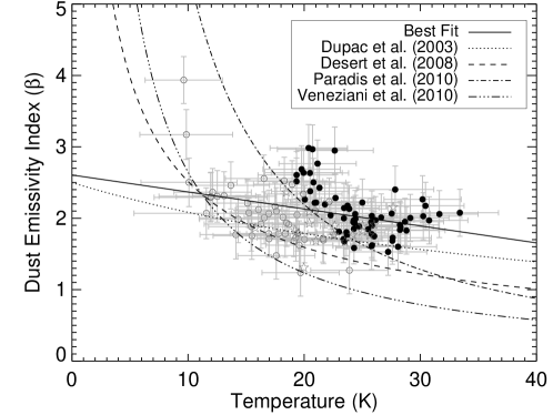
Figure 10: The $\beta$-$T_{d}$ relationship derived from the aperture photometry. Data points from the “warm” group are shown with filled circles while those from the “cold” group are shown with open circles. Data points from “PS” apertures are shown with star symbols. We plot on top of the data the best fit line as well as the best fits lines found by Dupac et al. (2003), Désert et al. (2008), Paradis et al. (2010), and Veneziani et al. (2010).

5.2.1 Simulations of the $\beta-T_{d}$ Relationship

We perform simulations to better understand the effect of calibration and photometric uncertainties on the derived $T_{d}$ and $\beta$-values. According to their user manuals, the flux calibration for the PACS and SPIRE instruments is stable in time and the calibration for the photometric bands of a given detector is correlated. We model four different combinations of calibration errors: $+5\%$ for all PACS bands and $+5\%$ for all SPIRE bands, $+5\%$ for PACS and $-5\%$ for SPIRE, $-5\%$ for PACS and $+5\%$ for SPIRE, and $-5\%$ for PACS and $-5\%$ for SPIRE. We use $+5\%$ for all 870 $\,\mu{\rm m}$ calibration errors. We chose these values for the uncertainty estimates to assess how different combinations of uncertainties may affect the derivation of the $\beta-T$ relationship. The values are not necessarily consistant with the instrumental and photometric uncertainties discussed in more detail below. Anderson et al. (2012) found using Herschel data that the photometric uncertainties are in most cases dominated by the choice of background region. We did not rigorously estimate this source of uncertainty here but we assume that the values are similar to those in Anderson et al. (2012). For the photometric uncertainty, we take the average uncertainty they give for their photometry of H II regions: 7%, 10%, 11%, 13%, and 15% for the 70 $\,\mu{\rm m}$, 160 $\,\mu{\rm m}$, 250 $\,\mu{\rm m}$, 350 $\,\mu{\rm m}$, and 500 $\,\mu{\rm m}$ bands. We assume the photometric uncertainty at 100 $\,\mu{\rm m}$ is 10% and the error at 870 $\,\mu{\rm m}$ is 15%.

We simulate the emission from dust that has a range of temperatures from 10 to 35 K in steps of 5 K, in a manner similar to that of Shetty et al. (2009a). For this simulation we use a single $\beta$ value of 2.0. For each $\beta-T_{d}$ combination, we calculate the fluxes of a simulated gray-body SED. We then randomly extract values from Gaussian photometric error distributions with $1\sigma$-levels given above. We add the calibration uncertianties in quadrature to the photometric errors. The resultant synthetic SEDs have flux values varied by representative calibration and photometric uncertainties. We have 16 trials from the combinations of four wavelength options and four calibration options.

We show the results of this modeling in Figure 11 for the four trials with calibration errors of $+5\%$ for PACS and $-5\%$ for SPIRE. Each data point in Figure 11 represents the derived $T_{d}$ and $\beta$-values for a single simulated SED; there are 600 data points in total, 100 for each input temperature. Points sharing a common input temperature also share a common shade of gray. All four trials with difference calibration errors that share a wavelength combination have results similar to that shown in Figure 11, although the scatter in the data points is generally larger when the PACS and SPIRE calibration errors have inverse signs.

A number of points are evident in Figure 11. First, for each $\beta-T_{d}$ pair, a false relationship is produced. Secondly, a large number of wavelengths helps greatly in reducing the spread in the calculated values and the uncertainty in the derived fit. Excluding either the 70 $\,\mu{\rm m}$ or the 870 $\,\mu{\rm m}$ data results in $\sim 50\%$ larger fit uncertainties; excluding both wavelengths results in $\sim 100\%$ larger fit uncertainties in both $\beta$ and $T_{d}$. Finally, the most likely value found is that of the input value; there is no systematic offset between the derived and input $\beta-T_{d}$ pair.

Could the $\beta-T_{d}$ relationship be falsely produced by our analysis? To better assess the effect of the Herschel calibration and photometric uncertainties on our derived $T_{d}$ and $\beta$-values, we repeat the simulation above using as input temperatures the 129 temperature values from the $\beta$-fixed trial derived in the aperture photometry (see Table 3), and $\beta=2.0$. When constructing the simulated SEDs, we include data at the same wavelengths as were included in our 129 aperture photometry fits: 42 data points with 70 $\,\mu{\rm m}$ and 870 $\,\mu{\rm m}$ data, 2 data points with 70 $\,\mu{\rm m}$ but no 870 $\,\mu{\rm m}$ data, 16 data points with 870 $\,\mu{\rm m}$ data but no 70 $\,\mu{\rm m}$ data, and 69 data points with neither 70 $\,\mu{\rm m}$ nor 870 $\,\mu{\rm m}$ data. We use for the calibration errors one value for all PACS bands and one value for all SPIRE bands. This calibration error is drawn randomly from a uniform distribution, using as a maximum the percentage error given previously in Section 3. We treat the photometric errors in the same way as described above and again add these two sources of error in quadrature. We simulate the 129 SEDs 1, 000 times, using for each of the 1, 000 trials different calibration errors. We fit both a linear regression line and also a power law regression to each of the 1, 000 sets of 129 points.

In Figure 12 we show an example from one of the 1, 000 trials: the trial whose linear regression fit parameters are the closest to the median fit parameters from all 1, 000 trials. As in Figure 11, each data point in Figure 12 is the fit to a simulated SED that includes calibration and photometric errors. If there were no sources of error added, we would recover the 129 derived temperatures, all with $\beta=2.0$. The simulated temperature and $\beta$-values shown in Figure 12 are visually similar to our derived values shown in Figure 10. The median linear fit is:

$$\beta=2.6\pm 0.2-(0.02\pm 0.01)\,T_{d}\,,$$ (7)

and the median power-law fit is

$$\beta=(4.0\pm 1.3)\,T_{d}^{-0.2\pm 0.1}\,.$$ (8)

The simulated fits again show a weak inverse relationship between $\beta$ and $T_{d}$, with the same values (within the errors) as what was found in Equation 5 and Equation 6.

From Figures 10 and 12, there appears to be less variation in $\beta$ in the simulated data than in the real data. The summed square of the difference in $\beta$ between the linear fit and values of $\beta$ in Figure 10 is 15.6. The median summed squared difference in the 1, 000 fits to the synthetic data described above is 13.0 with a large standard deviation of 8.2. We therefore conclude that most of the variation in $\beta$ can be explained by calibration and photometric uncertainty but that there may also be variations in $\beta$ not explained by these sources of uncertainty.

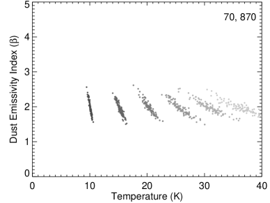
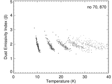
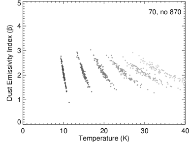
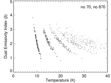
Figure 11: Fits of $T_{d}$ and $\beta$ using simulated data. Each data point is the result of an SED fit to simulated data accounting for calibration and photometric uncertainties. The simulated SEDs were created with input temperature values from 10 to 35 K in steps of 5 K and $\beta=2.0$. Points with a common input temperature share a common shade of gray.

Figure 12: Fits of $T_{d}$ and $\beta$ using simulated data, similar to Figure 11. We used the fitted temperatures from Table 3 to create the simulated data, and $\beta=2.0$. Shown is one of 1, 000 trials using different simulated calibration errors. Colors indicate the input temperature to the simulated SEDs: black is $\sim 10$ K and light gray is $\sim 35$ K.

5.2.2 Comparison with Previous Results Using These Data

The lack of a strong relationship between $T_{d}$ and $\beta$ is in contrast to the suggestion of Anderson et al. (2010) and Rodón et al. (2010). Using an earlier processing of the same data employed here for RCW 120 and Sh-104 (except for the Herschel Hi-Gal 70 $\,\mu{\rm m}$ data for RCW 120), these authors’ results were consistent with the existence of a relationship between $T_{d}$ and $\beta-T$, although these works did not consider the error simulations that we perform here. The methods between their works and ours are nearly identical and therefore it seems likely that the updated processing of the Herschel data has caused some of the differences. The median absolute flux differences between our processing and the processing used in Anderson et al. (2010) for RCW 120 (after rebinning to the same pixel grid and subtracting a background such that 99.99% of the pixels have positive values) are 2.3%, 4.7%, 0.7%, 0.7%, and 0.8% for the 100 $\,\mu{\rm m}$, 160 $\,\mu{\rm m}$, 250 $\,\mu{\rm m}$, 350 $\,\mu{\rm m}$, and 500 $\,\mu{\rm m}$ data. The median absolute flux differences for Sh-104 are similar: 0.8%, 1.2%, 0.4%, 0.3%, and 0.5% for the 100 $\,\mu{\rm m}$, 160 $\,\mu{\rm m}$, 250 $\,\mu{\rm m}$, 350 $\,\mu{\rm m}$, and 500 $\,\mu{\rm m}$ data.

The reprocessing has affected some derived values of $T_{\rm dust}$ and $\beta$, but these differences are generally within the previously stated uncertainties. Because we use Hi-Gal 70 $\,\mu{\rm m}$ data here in place of the MIPSGAL (Carey et al., 2009) 70 $\,\mu{\rm m}$ data used in Anderson et al. (2010) the differences in derived $T_{d}$ and $\beta$-values reflect the combined effect of the new processing (including changes to the calibration) and the different 70 $\,\mu{\rm m}$ data sets. For the trial when $\beta$ was allowed to vary, the median absolute temperature difference is 2.4 K. About half of the apertures in common have temperature values within the uncertainties given in Anderson et al. (2010). The median absolute difference in $\beta$ is 0.3, and over half of these differences are within the uncertainties given in Anderson et al. (2010). The data used here for Sh-104 are the same as that of Rodón et al. (2010), albiet reprocessed. We find that, for the trial when $\beta$ was free to vary, the median absolute difference in temperature between what we find here and that shown in Rodón et al. (2010) is 1.2 K; in all cases this median absolute temperature difference is less than the errors given in Rodón et al. (2010). The median absolute difference in $\beta$-value is 0.2 and for all apertures except for two the differences are less than the errors given in Rodón et al. (2010).

So why does our interpretation of the $\beta-T_{d}$ relationship differ from that of Anderson et al. (2010) and Rodón et al. (2010)? Both of their results were based on 15 apertures from one field while our result here is based on 129 apertures from eight fields; we believe our results are more robust. Additionally, their $\beta-T_{d}$ fits were dependant on results toward the “interior” of the bubbles, which we have excluded from the present analysis. Our thinking has evolved on the issue of the bubble interiors and, given the range of dust temperatures likely present there (see Section 5.4), it seems prudent to exclude the interiors from any analysis involving single-temperature fits. We note that the temperatures for the “interior” apertures in Rodón et al. (2010) have significantly higher uncertainties than those of other apertures in the field. We conclude that the differences between the present work and the previous analyses stem partly from differences in data processing, but also from which apertures were considered and which 70 $\,\mu{\rm m}$ data were used. This demonstrates the caution required for future work on the $\beta-T_{d}$ relationship.

5.3 The Three-Dimensional Nature of Bubbles

There has recently been some debate on whether the types of H II  regions studied here are two-dimensional objects, “rings,” or three-dimensional objects, “bubbles.” The $J=3\rightarrow 2$ ${}^{\rm 12}{\rm CO}$  observations in Beaumont & Williams (2010) show little emission toward the bubble interiors. The lack of detected CO emission in the bubble interiors indicates that “bubbles” are flat objects. Anderson et al. (2011), however, suggest that bipolar bubbles would be much more common if all bubbles were two-dimensional, an effect that is not observed. Furthermore, these authors point out that the recombination line widths of bubbles that are not bi-polar should be larger since the ionized flows toward and away from the observer are largely unimpeeded; such larger line widths are not observed.

The Herschel data shown here also support the idea that bubble H II regions are three-dimensional structures. Toward the center of all bubbles in our sample there is emission at all Herschel wavelengths. While at wavelengths $<\!100\,\,\mu{\rm m}$, such emission comes mainly from a warmer dust component (see below), the longer wavelength emission indicates the presense of cold dust. If such bubbles were in fact rings, we would not expect to find cold dust toward their central regions. Anderson et al. (2010) found support for the hypothesis of Beaumont & Williams (2010) - namely little emission toward center of RCW 120. This observation, however, relied on an earlier processing of the Herschel data that removed emission around bright PDRs and thus from the bubble interiors. The current processing using Scanamorphos better reconstructs the flux around and within the bubble interiors.

What percentage of the total emission comes from the bubble interiors? Using aperture photometry, we answer this question by comparing the flux from the bubble interiors against that of the “Entire” class defined earlier. The four angularly largest regions in our sample, Sh 104, W5-E, RCW 79, and RCW 120 permit the most accurate measurements, and we restrict the current analysis to these regions. We use the “Entire” apertures from earlier and define new apertures at each wavelength for the interior regions that trace the inner PDR boundary. Because the choice of background aperture may affect our measurements, we define four background apertures for each wavelength of the four H II regions. We perform the aperture photometry as before to determine the percentage of the total emission detected towards the bubble “interiors.”

Roughly $20\%$ of the total emission from the bubbles in our sample comes from the interior. This indicates that toward the interior of the bubbles, we are detecting cold dust emission from the “front” and “back” sides of the bubble. The average percentage of emission from the interior for the four regions studied here at 100 $\,\mu{\rm m}$, 160 $\,\mu{\rm m}$, 250 $\,\mu{\rm m}$, 350 $\,\mu{\rm m}$ and 500 $\,\mu{\rm m}$ is $26\pm 0.7\%$, $20\pm 6\%$, $17\pm 7\%$, $14\pm 8\%$, and $12\pm 7\%$, respectively. Much of the deviation in the above numbers comes from Sh 104, which has 10% more flux from the interior at each wavelength compared to the averages. The exact interpretation of these numbers requires modeling that is beyond the scope of this paper. It is, nevertheless, suggestive that some bubble H II regions are three-dimensional objects.

A higher percentage of the emission at lower wavelengths comes from the bubble interiors. Restricting our analysis to RCW 79 and RCW 120, for which we have Herschel Hi-Gal observations at 70 $\,\mu{\rm m}$ and MIPSGAL observations at 24 $\,\mu{\rm m}$, we find that the contribution to the total flux from the interior is 60% at 24 $\,\mu{\rm m}$ for RCW 120 and 55% for RCW 79, and 33% at 70 $\,\mu{\rm m}$ for RCW 120 and 69% for RCW 79. These 24 $\,\mu{\rm m}$ values are slightly higher than that of Deharveng et al. (2010), who found that about half the emission at 24 $\,\mu{\rm m}$ comes from the bubble interiors.

5.4 The Warm Dust Component

Nearly all regions in our sample have a “warm” dust component not accounted for in the current treatment (see Figure 7). This component has significantly less flux compared to the cold component. For a given flux, the mass decreases with increasing temperature. The lower flux and higher temperature together imply that the warm component contains very little mass compared to the cold component. The warm component emits strongly at 24 $\,\mu{\rm m}$ for bubble H II regions (see Watson et al., 2008; Deharveng et al., 2010), but Herschel observations also show emission at longer wavelengths, especially 70 $\,\mu{\rm m}$ and 100 $\,\mu{\rm m}$, with the same spatial distribution seen at 24 $\,\mu{\rm m}$ (Figure 13). This indicates that some fraction of the emission in the Herschel PACS bands is due to the warm component. This warm component has generally been attributed to stochastically heated very small grains (VSGs; Draine & Li, 2007).

Figure 13: The warm dust component in RCW 79. The warm dust is prominent at 24 $\,\mu{\rm m}$ and decreases in intensity relative to the emission from the PDR at longer wavelengths. The size of all fields is $20\arcmin$ square.

Using the dust model DustEM (Compiègne et al., 2011), Compiègne et al. (2010) show the SED Herschel Hi-Gal field at $\ell=59\degr$, a “diffuse” region and a “dense” region. In the “diffuse” field they found that the VSG component contributes on average $35\%$ of the flux at 70 $\,\mu{\rm m}$, 13% of the flux at 100 $\,\mu{\rm m}$, and 5% of the flux at 160 $\,\mu{\rm m}$. In the “dense” field, these percentages decreased to 12%, 4%, and 2%, respectively. Neither region contains active star formation. Since nearly all of our measurements are toward dense structures, it seems likely that the latter numbers are more representative of our data.

What effect does including data at 70 $\,\mu{\rm m}$ have on our derived temperatures? Of the data used here to derive dust temperatures, the 70 $\,\mu{\rm m}$ data are most heavily affected by a possible warmer dust contribution, caused in part by the emission from VSGs. To answer this question, we perform two tests. In the first test, we recompute the temperature map for RCW 120 including the 70 $\,\mu{\rm m}$ data, and compare it to the map computed without the 70 $\,\mu{\rm m}$ data. We find that including or excluding the 70 $\,\mu{\rm m}$ data point has minimal impact on the derived temperatures: the average change per temperature map pixel is $\sim 4\%$, or 1.6 K on average. In our second test, we re-fit the fluxes extracted with aperture photometry for RCW 120. The temperatures change by $\sim 6\%$ on average for RCW 120 apertures, compared to the temperatures derived when the 70 $\,\mu{\rm m}$ data are included when $\beta$ is held to a value of 2.0. When $\beta$ is allowed to vary, the derived temperatures change by $\sim 4\%$ and the derived $\beta$ values change by $\sim 8\%$. In both cases, excluding the 70 $\,\mu{\rm m}$ data has the effect of decreasing the derived temperature by $<1$ K on average, although the derived $\beta$-values are on average neither higher nor lower. Excluding data at 70 $\,\mu{\rm m}$, however, increases the fit uncertainties (cf. Figure 11). We conclude that including data at 70 $\,\mu{\rm m}$ data has minimal impact on the derived temperatures and $beta$-values.

We stress that the impact of excluding the 70 $\,\mu{\rm m}$ is lessened because we also have data at 100 $\,\mu{\rm m}$. We re-fit the fluxes extrated using aperture photometry for RCW 120 excluding data at both 70 $\,\mu{\rm m}$ and 100 $\,\mu{\rm m}$. When $\beta$ is held fixed to a value of 2.0, we find temperatures $\sim 40\%$ different than when the 70 $\,\mu{\rm m}$ and 100 $\,\mu{\rm m}$ data were included. For apertures with previously-derived temperatures greater than $30$ K, the temperature difference is up to 100%. Many regions of the Hi-Gal survey will not have access to Herschel data at 100 $\,\mu{\rm m}$. We caution that the derived temperatures for regions $>30$ K will not be well-constrained if 70 $\,\mu{\rm m}$ data are excluded and 100 $\,\mu{\rm m}$ data are not available.

What effect may the warmer dust component have on our derived temperatures? To answer this question, we re-fit the data for RCW 120 after decreasing the flux to account for the warmer dust. To account for the largest possible contribution, we adjusted the fluxes downward by the average values for the diffuse field in Compiègne et al. (2010) (35%, 13%, and 5% for 70 $\,\mu{\rm m}$, 100 $\,\mu{\rm m}$, and 160 $\,\mu{\rm m}$) and re-fit the SED. We find that the derived temperatures change by $\sim 5\%$ both when $\beta$ is fixed and when it is allowed to vary, and that the derived $\beta$-values change by $\sim 5\%$. As mentioned above, these probably over-estimate any contribution from a warmer dust component for the dense structures here studied, and therefore the 5% temperature change should be regarded as an upper limit. We conclude that the warmer dust component, caused in part by VSGs, has minimal effect on the derived temperatures and $\beta$-values.

5.5 The Masses of Bubble HII Regions

The collect and collapse process requires a massive shell of material for the formation of second-generation stars. With the calculated masses, we may test whether the derived mass is similar to that expected based on the size of the region. We show in Figure 14 the relationship between the total mass of the H II region from the “Entire” apertures and the expected mass based on the physical size of the region, for a range of ambient densities from 100 to 1, 000 cm^-3. We calculated the expected mass by assuming that all material overtaken by the ionization front during the expansion of the H II region is still associated with the region, by neglecting the mass from the ionized plasma, and by assuming that the H II regions are spherical. The expected mass is therefore the dust density times the volume of the sphere times a gas-to-dust ratio of 100 (the bubble diameters are given in Table 1). The assumption that the bubbles are spherically symmetric introduces uncertainty to the calculations. It is nevertheless a good first-order assumption and is supported by our finding that the bubbles are likely three-dimensional (see Section 5.3).

Figure 14 shows that for most regions, the computed mass is similar to the expected mass for reasonable values of the ambient density. The largest exception is for W5-E, which has significantly less mass than expected. The expansion of W5-E may not have been restricted, as is implied by its open geometry. This region may have formed in a filament oriented east-west, and its expansion to the north and south may have progressed largely unimpeded (Deharveng et al., 2012). The opposite may be the case for RCW 71 and G332, which have more mass than expected and appear to have nearly complete PDRs.

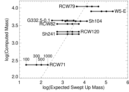
Figure 14: The expected swept up mass versus the calculated mass for the eight bubble regions. The expected mass is computed for initial ambient densities from 100 to 1, 000 cm^-3, assuming all material overtaken by the ionization front is now contained in the PDR of the region. The dashed line shows a one-to-one relationship.

6 Conclusions

We have analyzed the dust properties of eight Galactic H II regions with a bubble morphology using Herschel data from the HOBYS and “Evolution of Interstellar Dust” key programs. We used aperture photometry to determine the dust temperature and dust emissivity index $\beta$ for regions of interest within the fields of these eight regions. We also computed maps of the dust temperature and the total column density. Most locations show contributions from two dust components. Here we only determine temperatures for the colder of these two components, which contains nearly all the dust mass.

Our conclusions are:

• All H II regions in the sample are well-characterized with mean dust temperatures of 26 K.

• The PDRs of the H II regions have mean temperatures of 26 K. The temperature is an important parameter for investigating subsequent star formation since higher temperatures lead to higher values of the Jeans mass, all else being equal. At the wavelengths sampled by Herschel, bubble H II regions are dominated by the emission from their PDRs – approximately 80% of the total flux is contained within the PDR. The remaining 20% of the flux is from the interior of the bubbles, which suggests that the bubbles are three-dimensional structures rather than rings.

• The apertures can be divided into two statistically distinct groups: a “warm” group averaging 26 K and a cold group averaging 17 K. The “warm” group contains apertures from the PDRs of H II regions, as well as the total emission from the H II regions themselves while the “cold” group contains apertures from cold filaments.

• The coldest regions of the fields are spatially coincident with infrared dark clouds (IRDCs); these have mean dust temperatures of 15 K. One third of the IRDCs here detected by Herschel have 160 $\,\mu{\rm m}$ fluxes greater than their 100 $\,\mu{\rm m}$ fluxes. This criterion can be used to locate clouds with similar temperatures that, because of the lack of mid-infrared background, do not appear infrared dark. Filaments that are not detect in absorption at 8.0 $\,\mu{\rm m}$ have mean dust temperatures of 19 K.

• We estimate that not accounting for the warmer dust component and including the data at 70 $\,\mu{\rm m}$ affects the derived temperatures by at most 5% for the objects studied here. We stress that the inclusion of data at 70 $\,\mu{\rm m}$ has less of an impact because we also have data at 100 $\,\mu{\rm m}$ – the exclusion of data at both 70 $\,\mu{\rm m}$ and 100 $\,\mu{\rm m}$ results in large differences in temperature of $\sim 40\%$. This will be the situation for the majority of the Herschel Hi-Gal observations. In this case, the inclusion of data at 70 $\,\mu{\rm m}$ is preferable to its exclusion. Color corrections employed here change the derived temperatures by $\sim 3\%$.

• The total mass associated with these regions spans a wide range, from $\sim 300$ to $\sim 10,\,000$ $\,M_{\odot}$.

• We find only weak support for a relationship between $\beta$ and $T_{d}$, in contrast to what has been found by previous authors. The slight correlation between $\beta$ and $T_{d}$ that we found is statistically similar to that caused by calibration and photometric uncertainties. This result differs from what was suggested by earlier analyses of the data shown here, reduced using a different processing method. That the $\beta-T_{d}$ relationship is so sensitive to the data processing method shows the difficulty in trying to understand it using Herschel data alone.

Table 5: Dust properties derived from aperture photometry

$\beta=2$

$\beta$ free

Region

Name

$l$

$b$

Size

$T_{d}$

$M$

$T_{d}$

$\beta$

$M$

Class.

deg.

deg.

$\arcmin^{2}$

K

$\,M_{\odot}$

K

$\,M_{\odot}$

Sh 104

Entire

74.765

$+0.624$

$75.0$

$24.4\pm 0.8$

$4200$

$27.6\pm 3.9$

$1.7\pm 0.3$

$3300$

E

HII (UCHII)

74.790

$+0.572$

$\phantom{0}2.7$

$28.1\pm 1.0$

$\phantom{0}440$

$28.7\pm 4.2$

$2.0\pm 0.3$

$\phantom{0}420$

H II

CS (CS)

74.721

$+0.590$

$\phantom{0}0.5$

$24.1\pm 0.7$

$\phantom{0}\phantom{0}89$

$25.0\pm 3.2$

$1.9\pm 0.3$

$\phantom{0}\phantom{0}82$

PS

E. PDR

74.766

$+0.565$

$\phantom{0}1.2$

$24.9\pm 0.8$

$\phantom{0}140$

$24.4\pm 3.0$

$2.1\pm 0.3$

$\phantom{0}150$

PDR

N. PDR 1 (PDR 2)

74.812

$+0.615$

$\phantom{0}0.9$

$22.2\pm 0.6$

$\phantom{0}120$

$23.6\pm 2.8$

$1.8\pm 0.3$

$\phantom{0}110$

PDR

N. PDR 2 (PDR 3)

74.818

$+0.657$

$\phantom{0}2.0$

$24.0\pm 0.7$

$\phantom{0}110$

$24.3\pm 3.0$

$2.0\pm 0.3$

$\phantom{0}110$

PDR

W. PDR 1 (PDR 4)

74.787

$+0.679$

$\phantom{0}2.6$

$21.3\pm 0.6$

$\phantom{0}300$

$23.4\pm 2.7$

$1.7\pm 0.3$

$\phantom{0}240$

PDR

W. PDR 2 (PDR 6)

74.728

$+0.671$

$\phantom{0}2.4$

$23.8\pm 0.7$

$\phantom{0}160$

$24.7\pm 3.1$

$1.9\pm 0.3$

$\phantom{0}150$

PDR

S. PDR 1 (PDR 7)

74.706

$+0.624$

$\phantom{0}1.4$

$25.0\pm 0.8$

$\phantom{0}160$

$23.9\pm 2.9$

$2.1\pm 0.3$

$\phantom{0}170$

PDR

S. PDR 2 (PDR 8)

74.736

$+0.565$

$\phantom{0}1.2$

$26.7\pm 0.9$

$\phantom{0}\phantom{0}49$

$26.6\pm 3.7$

$2.0\pm 0.3$

$\phantom{0}\phantom{0}50$

PDR

N. Filament 1

74.865

$+0.705$

$\phantom{0}0.8$

$15.0\pm 0.5$

$\phantom{0}\phantom{0}31$

$13.7\pm 2.2$

$2.5\pm 0.9$

$\phantom{0}\phantom{0}41$

F

N. Filament 2

74.822

$+0.704$

$\phantom{0}2.4$

$18.1\pm 0.4$

$\phantom{0}180$

$18.5\pm 1.7$

$1.9\pm 0.3$

$\phantom{0}170$

F

N. Filament 3

74.843

$+0.618$

$\phantom{0}1.3$

$17.9\pm 0.4$

$\phantom{0}110$

$19.3\pm 1.9$

$1.7\pm 0.3$

$\phantom{0}\phantom{0}89$

F

N. Filament 4* (PDR 1)

74.836

$+0.583$

$\phantom{0}2.2$

$19.9\pm 0.5$

$\phantom{0}170$

$21.6\pm 2.3$

$1.7\pm 0.3$

$\phantom{0}140$

F

N. Filament 5*

74.767

$+0.783$

$\phantom{0}0.8$

$16.9\pm 0.6$

$\phantom{0}\phantom{0}22$

$17.8\pm 3.2$

$1.8\pm 0.8$

$\phantom{0}\phantom{0}19$

F

S. Filament 1*

74.670

$+0.566$

$\phantom{0}7.4$

$21.6\pm 0.6$

$\phantom{0}180$

$20.9\pm 2.5$

$2.1\pm 0.4$

$\phantom{0}190$

F

S. Filament 2* (Outer)

74.662

$+0.662$

$\phantom{0}1.7$

$14.8\pm 0.8$

$\phantom{0}\phantom{0}39$

$15.5\pm 3.4$

$1.8\pm 1.2$

$\phantom{0}\phantom{0}35$

F

W5-E

Entire

138.060

$+1.461$

$2515.3$

$23.8\pm 0.7$

$8000$

$24.2\pm 3.0$

$1.9\pm 0.3$

$7700$

E

HII 1 (Sh 201)

138.481

$+1.637$

$\phantom{0}\phantom{0}69.6$

$26.9\pm 0.9$

$\phantom{0}830$

$28.3\pm 4.1$

$1.9\pm 0.3$

$\phantom{0}750$

H II

HII 2

137.696

$+1.533$

$\phantom{0}\phantom{0}25.1$

$24.9\pm 0.8$

$\phantom{0}590$

$25.8\pm 3.4$

$1.9\pm 0.3$

$\phantom{0}550$

H II

HII 3

137.735

$+1.458$

$\phantom{0}\phantom{0}23.8$

$23.8\pm 0.7$

$\phantom{0}690$

$26.0\pm 3.4$

$1.8\pm 0.3$

$\phantom{0}580$

H II

E. PS 1

138.323

$+1.509$

$\phantom{0}\phantom{0}\phantom{0}2.4$

$21.0\pm 0.6$

$\phantom{0}\phantom{0}43$

$22.6\pm 2.5$

$1.8\pm 0.3$

$\phantom{0}\phantom{0}37$

PS

E. PS 2 (BRC14)

138.298

$+1.560$

$\phantom{0}\phantom{0}\phantom{0}4.4$

$23.5\pm 0.7$

$\phantom{0}440$

$25.6\pm 3.3$

$1.8\pm 0.3$

$\phantom{0}370$

PS

N. PS 1 (BRC13)

138.142

$+1.684$

$\phantom{0}\phantom{0}\phantom{0}1.6$

$22.4\pm 0.6$

$\phantom{0}\phantom{0}60$

$24.2\pm 2.9$

$1.8\pm 0.3$

$\phantom{0}\phantom{0}51$

PS

W. PS 1

137.793

$+1.461$

$\phantom{0}\phantom{0}\phantom{0}1.7$

$23.4\pm 0.7$

$\phantom{0}\phantom{0}49$

$25.0\pm 3.1$

$1.8\pm 0.3$

$\phantom{0}\phantom{0}43$

PS

W. PS 2 (BRC12)

137.505

$+1.397$

$\phantom{0}\phantom{0}\phantom{0}1.3$

$21.9\pm 0.6$

$\phantom{0}\phantom{0}18$

$22.6\pm 2.6$

$1.9\pm 0.3$

$\phantom{0}\phantom{0}17$

PS

W. PS 3 (BRC12)

137.537

$+1.276$

$\phantom{0}\phantom{0}\phantom{0}1.5$

$21.2\pm 0.6$

$\phantom{0}\phantom{0}40$

$23.5\pm 2.7$

$1.7\pm 0.3$

$\phantom{0}\phantom{0}32$

PS

E. PDR 1 (BRC14)

138.308

$+1.568$

$\phantom{0}\phantom{0}23.0$

$22.6\pm 0.7$

$\phantom{0}770$

$25.8\pm 3.4$

$1.6\pm 0.3$

$\phantom{0}580$

PDR

E. PDR 2

138.319

$+1.671$

$\phantom{0}\phantom{0}\phantom{0}3.7$

$21.9\pm 0.6$

$\phantom{0}\phantom{0}54$

$23.7\pm 2.8$

$1.8\pm 0.3$

$\phantom{0}\phantom{0}46$

PDR

N. PDR 1 (BRC13)

138.187

$+1.727$

$\phantom{0}\phantom{0}24.7$

$21.6\pm 0.6$

$\phantom{0}400$

$23.0\pm 2.6$

$1.8\pm 0.3$

$\phantom{0}350$

PDR

N. PDR 2

138.031

$+1.762$

$\phantom{0}\phantom{0}\phantom{0}3.9$

$22.5\pm 0.6$

$\phantom{0}\phantom{0}27$

$21.0\pm 2.2$

$2.2\pm 0.3$

$\phantom{0}\phantom{0}32$

PDR

N. PDR 3

137.921

$+1.664$

$\phantom{0}\phantom{0}19.2$

$21.2\pm 0.6$

$\phantom{0}170$

$24.3\pm 2.9$

$1.6\pm 0.3$

$\phantom{0}130$

PDR

N. PDR 4

137.897

$+1.920$

$\phantom{0}\phantom{0}43.2$

$21.7\pm 0.6$

$\phantom{0}160$

$20.1\pm 2.0$

$2.3\pm 0.3$

$\phantom{0}200$

PDR

W. PDR 1

137.930

$+1.119$

$\phantom{0}196.1$

$23.1\pm 0.7$

$1100$

$24.3\pm 3.0$

$1.9\pm 0.3$

$1000$

PDR

W. PDR 2 (BRC12)

137.553

$+1.344$

$\phantom{0}\phantom{0}\phantom{0}6.9$

$23.8\pm 0.7$

$\phantom{0}\phantom{0}67$

$24.3\pm 3.0$

$1.9\pm 0.3$

$\phantom{0}\phantom{0}64$

PDR

N. Filament 1

138.256

$+1.850$

$\phantom{0}\phantom{0}\phantom{0}1.1$

$18.4\pm 0.4$

$\phantom{0}\phantom{0}\phantom{0}7.6$

$19.4\pm 2.0$

$1.8\pm 0.4$

$\phantom{0}\phantom{0}\phantom{0}6.6$

F

N. Filament 2

137.738

$+1.919$

$\phantom{0}\phantom{0}\phantom{0}5.4$

$15.8\pm 0.3$

$\phantom{0}\phantom{0}54$

$17.0\pm 1.4$

$1.7\pm 0.4$

$\phantom{0}\phantom{0}45$

F

E. Filament 1

138.596

$+1.707$

$\phantom{0}\phantom{0}12.4$

$17.5\pm 0.4$

$\phantom{0}\phantom{0}67$

$19.1\pm 1.8$

$1.7\pm 0.3$

$\phantom{0}\phantom{0}54$

F

E. Filament 2

138.594

$+1.584$

$\phantom{0}\phantom{0}\phantom{0}4.7$

$18.3\pm 0.4$

$\phantom{0}\phantom{0}79$

$18.7\pm 1.7$

$1.9\pm 0.3$

$\phantom{0}\phantom{0}75$

F

Sh 241

Entire

180.886

$+4.114$

$16.5$

$22.9\pm 0.7$

$1800$

$27.2\pm 3.8$

$1.5\pm 0.3$

$1300$

E

HII

180.828

$+3.993$

$\phantom{0}2.6$

$24.8\pm 0.8$

$\phantom{0}350$

$27.6\pm 3.9$

$1.7\pm 0.3$

$\phantom{0}290$

H II

N. PS*

180.820

$+4.189$

$\phantom{0}0.4$

$19.2\pm 0.5$

$\phantom{0}\phantom{0}32$

$21.0\pm 2.2$

$1.7\pm 0.3$

$\phantom{0}\phantom{0}26$

PS

W. PS*

180.859

$+4.032$

$\phantom{0}0.5$

$16.6\pm 0.4$

$\phantom{0}\phantom{0}93$

$20.0\pm 1.9$

$1.3\pm 0.3$

$\phantom{0}\phantom{0}58$

PS

S. PS*

180.918

$+4.017$

$\phantom{0}0.9$

$18.4\pm 0.4$

$\phantom{0}110$

$19.5\pm 1.9$

$1.8\pm 0.3$

$\phantom{0}\phantom{0}98$

PS

N. PDR 1

180.856

$+4.122$

$\phantom{0}0.8$

$23.8\pm 0.7$

$\phantom{0}150$

$25.8\pm 3.4$

$1.8\pm 0.3$

$\phantom{0}130$

PDR

N. PDR 2

180.858

$+4.106$

$\phantom{0}0.7$

$24.1\pm 0.8$

$\phantom{0}150$

$28.1\pm 4.0$

$1.6\pm 0.3$

$\phantom{0}110$

PDR

W. PDR

180.873

$+4.092$

$\phantom{0}1.3$

$22.5\pm 0.7$

$\phantom{0}560$

$25.8\pm 3.3$

$1.6\pm 0.3$

$\phantom{0}420$

PDR

W. Filament 1*

180.855

$+4.069$

$\phantom{0}0.4$

$19.2\pm 0.5$

$\phantom{0}\phantom{0}39$

$23.9\pm 3.3$

$1.3\pm 0.4$

$\phantom{0}\phantom{0}24$

F

W. Filament 2*

180.840

$+4.044$

$\phantom{0}5.4$

$18.5\pm 0.4$

$\phantom{0}540$

$20.0\pm 2.0$

$1.7\pm 0.3$

$\phantom{0}450$

F

W. Filament 3*

180.866

$+4.053$

$\phantom{0}0.3$

$15.4\pm 0.3$

$\phantom{0}110$

$17.6\pm 1.6$

$1.5\pm 0.4$

$\phantom{0}\phantom{0}79$

F

W. Filament 4*

180.874

$+4.047$

$\phantom{0}0.7$

$16.1\pm 0.4$

$\phantom{0}140$

$19.7\pm 1.9$

$1.2\pm 0.3$

$\phantom{0}\phantom{0}82$

F

S. Filament*

180.915

$+4.040$

$\phantom{0}0.9$

$17.3\pm 0.4$

$\phantom{0}100$

$18.4\pm 1.9$

$1.8\pm 0.4$

$\phantom{0}\phantom{0}87$

F

RCW 71

Entire

302.799

$+1.287$

$21.6$

$30.3\pm 1.2$

$240$

$30.8\pm 5.0$

$2.0\pm 0.3$

$230$

E

S. PS 1*

302.842

$+1.225$

$\phantom{0}0.8$

$15.3\pm 0.3$

$\phantom{0}37$

$15.8\pm 1.4$

$1.9\pm 0.4$

$\phantom{0}34$

PS

S. PS 2*

302.809

$+1.233$

$\phantom{0}0.9$

$18.2\pm 0.4$

$\phantom{0}20$

$19.2\pm 2.0$

$1.8\pm 0.4$

$\phantom{0}18$

PS

N. PDR

302.802

$+1.309$

$\phantom{0}1.6$

$34.5\pm 1.6$

$\phantom{0}13$

$30.2\pm 5.0$

$2.3\pm 0.4$

$\phantom{0}16$

PDR

W. PDR

302.780

$+1.284$

$\phantom{0}0.7$

$30.7\pm 1.2$

$\phantom{0}15$

$30.2\pm 4.9$

$2.0\pm 0.3$

$\phantom{0}15$

PDR

S. PDR 1

302.784

$+1.259$

$\phantom{0}1.1$

$28.3\pm 1.0$

$\phantom{0}20$

$27.5\pm 4.0$

$2.1\pm 0.3$

$\phantom{0}21$

PDR

S. PDR 2

302.807

$+1.261$

$\phantom{0}0.8$

$26.4\pm 0.9$

$\phantom{0}24$

$28.2\pm 4.1$

$1.8\pm 0.3$

$\phantom{0}21$

PDR

E. PDR 1

302.822

$+1.291$

$\phantom{0}0.6$

$34.9\pm 1.7$

$\phantom{0}\phantom{0}8.7$

$33.4\pm 6.2$

$2.1\pm 0.4$

$\phantom{0}\phantom{0}9.3$

PDR

E. PDR 2

302.810

$+1.277$

$\phantom{0}0.6$

$33.2\pm 1.5$

$\phantom{0}19$

$30.4\pm 4.9$

$2.2\pm 0.3$

$\phantom{0}22$

PDR

E. PDR 3

302.823

$+1.273$

$\phantom{0}0.5$

$32.6\pm 1.4$

$\phantom{0}\phantom{0}6.9$

$31.6\pm 5.6$

$2.1\pm 0.4$

$\phantom{0}\phantom{0}7.3$

PDR

W. Filament 1*

302.718

$+1.319$

$\phantom{0}2.3$

$16.1\pm 0.4$

$\phantom{0}40$

$16.9\pm 1.6$

$1.8\pm 0.4$

$\phantom{0}35$

F

W. Filament 2*

302.732

$+1.307$

$\phantom{0}0.5$

$18.3\pm 0.5$

$\phantom{0}\phantom{0}5.8$

$18.2\pm 2.5$

$2.0\pm 0.6$

$\phantom{0}\phantom{0}6.0$

F

W. Filament 3*

302.720

$+1.271$

$\phantom{0}0.6$

$14.3\pm 0.3$

$\phantom{0}12$

$14.3\pm 1.7$

$2.0\pm 0.6$

$\phantom{0}12$

F

W. Filament 4*

302.734

$+1.276$

$\phantom{0}0.5$

$17.3\pm 0.4$

$\phantom{0}\phantom{0}8.9$

$16.9\pm 2.0$

$2.1\pm 0.5$

$\phantom{0}\phantom{0}9.3$

F

N. Filament*

302.859

$+1.388$

$\phantom{0}0.8$

$12.8\pm 0.6$

$\phantom{0}\phantom{0}9.8$

$9.6\pm 1.9$

$3.9\pm 1.6$

$\phantom{0}29$

F

RCW 79

Entire

308.709

$+0.628$

$182.4$

$26.9\pm 0.9$

$11000$

$28.8\pm 3.8$

$1.8\pm 0.3$

$9700$

E

HII

308.750

$+0.548$

$\phantom{0}\phantom{0}6.8$

$27.5\pm 0.9$

$\phantom{0}1700$

$25.0\pm 2.0$

$2.2\pm 0.2$

$2100$

H II

W. PS 1 (Cond. 4)

308.645

$+0.648$

$\phantom{0}\phantom{0}1.4$

$25.1\pm 0.8$

$\phantom{0}\phantom{0}720$

$26.0\pm 2.4$

$1.9\pm 0.2$

$\phantom{0}660$

PS

W. PS 2 (Cond. 6)

308.673

$+0.637$

$\phantom{0}\phantom{0}1.1$

$29.7\pm 1.1$

$\phantom{0}\phantom{0}\phantom{0}73$

$27.7\pm 3.1$

$2.2\pm 0.2$

$\phantom{0}\phantom{0}84$

PS

N. PDR 1 (Cond. 5)

308.729

$+0.725$

$\phantom{0}\phantom{0}2.6$

$23.4\pm 0.6$

$\phantom{0}\phantom{0}440$

$21.8\pm 1.7$

$2.2\pm 0.2$

$\phantom{0}520$

PDR

N. PDR 2

308.793

$+0.648$

$\phantom{0}14.0$

$29.2\pm 1.0$

$\phantom{0}\phantom{0}660$

$21.1\pm 1.6$

$2.8\pm 0.2$

$1300$

PDR

W. PDR 1

308.630

$+0.558$

$\phantom{0}\phantom{0}3.6$

$34.3\pm 1.5$

$\phantom{0}\phantom{0}170$

$27.8\pm 2.9$

$2.4\pm 0.2$

$\phantom{0}250$

PDR

W. PDR 2

308.613

$+0.607$

$\phantom{0}\phantom{0}4.2$

$36.1\pm 1.6$

$\phantom{0}\phantom{0}250$

$22.6\pm 1.8$

$2.9\pm 0.2$

$\phantom{0}610$

PDR

W. PDR 3 (Cond. 7)

308.673

$+0.620$

$\phantom{0}\phantom{0}0.9$

$27.1\pm 1.0$

$\phantom{0}\phantom{0}\phantom{0}69$

$28.2\pm 3.2$

$1.9\pm 0.2$

$\phantom{0}\phantom{0}64$

PDR

S. PDR (Cond. 3)

308.690

$+0.533$

$\phantom{0}\phantom{0}6.6$

$25.2\pm 0.8$

$\phantom{0}1400$

$25.8\pm 2.3$

$1.9\pm 0.2$

$1300$

PDR

2nd PDR E.

308.708

$+0.470$

$\phantom{0}23.5$

$24.3\pm 0.7$

$\phantom{0}2000$

$24.4\pm 3.0$

$2.0\pm 0.3$

$2000$

PDR

2nd PDR W.

308.522

$+0.585$

$\phantom{0}14.7$

$23.1\pm 0.7$

$\phantom{0}\phantom{0}610$

$20.5\pm 2.1$

$2.4\pm 0.4$

$\phantom{0}800$

PDR

N. Filament (Cond. 8)

308.725

$+0.774$

$\phantom{0}\phantom{0}6.9$

$21.7\pm 0.5$

$\phantom{0}\phantom{0}950$

$18.3\pm 1.1$

$2.5\pm 0.2$

$1400$

F

E. Filament*

308.892

$+0.698$

$\phantom{0}\phantom{0}7.9$

$24.0\pm 0.7$

$\phantom{0}\phantom{0}130$

$22.1\pm 2.4$

$2.2\pm 0.3$

$\phantom{0}160$

F

RCW 82

Entire

310.980

$+0.408$

$62.2$

$24.6\pm 0.7$

$3400$

$21.3\pm 2.2$

$2.4\pm 0.3$

$4700$

E

E. PS

311.034

$+0.382$

$\phantom{0}1.8$

$21.1\pm 0.5$

$\phantom{0}430$

$20.4\pm 1.4$

$2.1\pm 0.2$

$\phantom{0}470$

PS

N. PDR 1

311.003

$+0.462$

$\phantom{0}2.2$

$25.3\pm 0.8$

$\phantom{0}200$

$22.7\pm 1.9$

$2.3\pm 0.2$

$\phantom{0}250$

PDR

W. PDR 1

310.948

$+0.424$

$\phantom{0}2.8$

$29.7\pm 1.0$

$\phantom{0}130$

$20.4\pm 1.9$

$3.0\pm 0.3$

$\phantom{0}280$

PDR

W. PDR 2

310.928

$+0.445$

$\phantom{0}2.1$

$25.8\pm 0.8$

$\phantom{0}190$

$20.5\pm 1.7$

$2.6\pm 0.3$

$\phantom{0}310$

PDR

S. PDR

310.987

$+0.359$

$\phantom{0}4.8$

$25.5\pm 0.7$

$\phantom{0}340$

$19.8\pm 1.4$

$2.7\pm 0.2$

$\phantom{0}590$

PDR

E. PDR 1

311.026

$+0.413$

$\phantom{0}1.5$

$25.3\pm 0.7$

$\phantom{0}160$

$19.9\pm 1.4$

$2.6\pm 0.2$

$\phantom{0}270$

PDR

E. PDR 2

311.013

$+0.430$

$\phantom{0}1.1$

$23.0\pm 0.6$

$\phantom{0}110$

$19.3\pm 1.4$

$2.5\pm 0.2$

$\phantom{0}160$

PDR

N. Filament*

311.060

$+0.516$

$\phantom{0}2.6$

$21.9\pm 0.6$

$\phantom{0}\phantom{0}79$

$19.0\pm 1.8$

$2.5\pm 0.4$

$\phantom{0}110$

F (ID)

W. Filament*

310.850

$+0.486$

$\phantom{0}4.0$

$18.4\pm 0.4$

$\phantom{0}260$

$17.5\pm 1.4$

$2.2\pm 0.3$

$\phantom{0}300$

F

S. Filament 1*

310.927

$+0.277$

$\phantom{0}2.7$

$18.0\pm 0.6$

$\phantom{0}\phantom{0}57$

$17.6\pm 2.3$

$2.1\pm 0.5$

$\phantom{0}\phantom{0}60$

F

S. Filament 2*

310.896

$+0.379$

$\phantom{0}2.5$

$19.3\pm 0.5$

$\phantom{0}\phantom{0}97$

$16.5\pm 1.6$

$2.6\pm 0.4$

$\phantom{0}140$

F (ID)

E. Filament 1*

311.086

$+0.429$

$\phantom{0}5.5$

$19.7\pm 0.5$

$\phantom{0}300$

$19.4\pm 1.5$

$2.0\pm 0.3$

$\phantom{0}310$

F

E. Filament 2*

311.052

$+0.394$

$\phantom{0}1.1$

$13.0\pm 0.3$

$\phantom{0}290$

$12.1\pm 0.9$

$2.4\pm 0.4$

$\phantom{0}380$

F (ID)

G332.5$-$0.1

Entire

332.539

$-0.141$

$13.6$

$25.9\pm 0.8$

$4500$

$26.1\pm 3.3$

$2.0\pm 0.3$

$4500$

E

HII 1

332.544

$-0.126$

$\phantom{0}0.9$

$29.2\pm 1.0$

$\phantom{0}590$

$29.1\pm 3.1$

$2.0\pm 0.2$

$\phantom{0}590$

UC

HII 2

332.445

$-0.178$

$\phantom{0}4.4$

$24.0\pm 0.7$

$\phantom{0}330$

$19.3\pm 1.4$

$2.6\pm 0.2$

$\phantom{0}540$

UC

W. PS

332.603

$-0.167$

$\phantom{0}1.6$

$20.0\pm 0.5$

$1200$

$20.4\pm 1.4$

$1.9\pm 0.2$

$1100$

PS

E. PS

332.467

$-0.130$

$\phantom{0}1.8$

$20.7\pm 0.5$

$\phantom{0}850$

$18.5\pm 1.2$

$2.4\pm 0.2$

$1100$

PS

E. PDR

332.560

$-0.149$

$\phantom{0}1.1$

$22.6\pm 0.6$

$\phantom{0}650$

$20.9\pm 1.5$

$2.2\pm 0.2$

$\phantom{0}770$

PDR

S. PDR

332.526

$-0.155$

$\phantom{0}1.4$

$25.5\pm 0.8$

$\phantom{0}650$

$23.7\pm 2.0$

$2.2\pm 0.2$

$\phantom{0}750$

PDR

E. Filament*

332.648

$-0.188$

$\phantom{0}3.2$

$15.9\pm 0.3$

$\phantom{0}700$

$15.1\pm 1.1$

$2.2\pm 0.3$

$\phantom{0}810$

F (ID)

S. Filament*

332.404

$-0.150$

$\phantom{0}5.0$

$19.6\pm 0.5$

$\phantom{0}820$

$21.7\pm 1.9$

$1.7\pm 0.3$

$\phantom{0}660$

F (ID)

W. Filament

332.501

$-0.119$

$\phantom{0}1.5$

$22.5\pm 0.6$

$\phantom{0}710$

$19.9\pm 1.3$

$2.3\pm 0.2$

$\phantom{0}930$

F (ID)

RCW 120

Entire

348.251

$+0.481$

$100.3$

$23.9\pm 0.6$

$2100$

$26.0\pm 2.4$

$1.7\pm 0.3$

$1800$

E

Cond. 1 PS

348.184

$+0.482$

$\phantom{0}\phantom{0}0.7$

$20.9\pm 0.5$

$\phantom{0}300$

$22.6\pm 1.6$

$1.8\pm 0.2$

$\phantom{0}260$

PS

Cond. 1 (Cond. 1)

348.180

$+0.480$

$\phantom{0}\phantom{0}4.7$

$21.0\pm 0.5$

$\phantom{0}760$

$23.5\pm 1.6$

$1.7\pm 0.2$

$\phantom{0}600$

PDR

S. PDR 1 (Cond. 2)

348.226

$+0.413$

$\phantom{0}\phantom{0}2.5$

$24.1\pm 0.6$

$\phantom{0}160$

$25.5\pm 2.0$

$1.8\pm 0.2$

$\phantom{0}140$

PDR

E. PDR 1 (Cond. 3)

348.272

$+0.403$

$\phantom{0}\phantom{0}2.6$

$23.4\pm 0.6$

$\phantom{0}\phantom{0}88$

$23.4\pm 1.9$

$2.0\pm 0.2$

$\phantom{0}\phantom{0}88$

PDR

E. PDR 2 (Cond. 4)

348.302

$+0.429$

$\phantom{0}\phantom{0}3.0$

$22.6\pm 0.6$

$\phantom{0}110$

$22.3\pm 1.7$

$2.0\pm 0.2$

$\phantom{0}110$

PDR

W. PDR 1 (Cond. 7)

348.199

$+0.531$

$\phantom{0}\phantom{0}0.7$

$24.8\pm 0.7$

$\phantom{0}\phantom{0}20$

$23.4\pm 1.9$

$2.1\pm 0.2$

$\phantom{0}\phantom{0}23$

PDR

S. PDR 1 (Cond. 10)

348.203

$+0.426$

$\phantom{0}\phantom{0}1.0$

$26.2\pm 0.8$

$\phantom{0}\phantom{0}38$

$25.8\pm 2.2$

$2.0\pm 0.2$

$\phantom{0}\phantom{0}39$

PDR

W. PDR 2 (PDR West)

348.266

$+0.556$

$\phantom{0}\phantom{0}0.8$

$31.6\pm 1.2$

$\phantom{0}\phantom{0}\phantom{0}6.0$

$20.7\pm 1.6$

$3.0\pm 0.2$

$\phantom{0}\phantom{0}14$

PDR

E. PDR 3 (PDR East)

348.329

$+0.464$

$\phantom{0}\phantom{0}1.2$

$25.3\pm 0.7$

$\phantom{0}\phantom{0}31$

$20.8\pm 1.4$

$2.5\pm 0.2$

$\phantom{0}\phantom{0}47$

PDR

W. IRDC 1*

348.179

$+0.600$

$\phantom{0}\phantom{0}1.5$

$12.7\pm 0.3$

$\phantom{0}\phantom{0}30$

$12.0\pm 0.9$

$2.3\pm 0.4$

$\phantom{0}\phantom{0}37$

F (ID)

W. IRDC 2*

348.165

$+0.662$

$\phantom{0}\phantom{0}2.3$

$14.0\pm 0.3$

$\phantom{0}\phantom{0}30$

$13.1\pm 0.8$

$2.3\pm 0.3$

$\phantom{0}\phantom{0}37$

F (ID)

W. IRDC 3*

348.196

$+0.768$

$\phantom{0}\phantom{0}1.8$

$13.5\pm 0.2$

$\phantom{0}\phantom{0}64$

$14.1\pm 1.1$

$1.8\pm 0.4$

$\phantom{0}\phantom{0}55$

F (ID)

W. IRDC 4*

348.234

$+0.591$

$\phantom{0}\phantom{0}1.8$

$17.6\pm 0.4$

$\phantom{0}\phantom{0}28$

$19.6\pm 2.0$

$1.6\pm 0.4$

$\phantom{0}\phantom{0}22$

F (ID)

N. IRDC 1* (Cond. 6)

348.292

$+0.644$

$\phantom{0}\phantom{0}2.0$

$15.0\pm 0.3$

$\phantom{0}160$

$15.4\pm 0.8$

$1.9\pm 0.2$

$\phantom{0}150$

F (ID)

N. IRDC 2* (Cond. 9)

348.345

$+0.652$

$\phantom{0}\phantom{0}1.5$

$13.4\pm 0.2$

$\phantom{0}110$

$12.5\pm 0.6$

$2.3\pm 0.2$

$\phantom{0}140$

F (ID)

N. IRDC 3*

348.297

$+0.682$

$\phantom{0}\phantom{0}1.4$

$13.1\pm 0.6$

$\phantom{0}\phantom{0}26$

$11.9\pm 1.5$

$2.3\pm 0.4$

$\phantom{0}\phantom{0}36$

F (ID)

N. IRDC 4*

348.305

$+0.703$

$\phantom{0}\phantom{0}0.8$

$12.2\pm 0.2$

$\phantom{0}\phantom{0}38$

$9.9\pm 0.4$

$3.2\pm 0.3$

$\phantom{0}\phantom{0}88$

F (ID)

N. IRDC 5*

348.325

$+0.716$

$\phantom{0}\phantom{0}1.4$

$11.5\pm 0.4$

$\phantom{0}\phantom{0}73$

$10.1\pm 1.1$

$2.5\pm 0.4$

$\phantom{0}120$

F (ID)

N. IRDC 6*

348.476

$+0.583$

$\phantom{0}\phantom{0}1.3$

$11.8\pm 0.5$

$\phantom{0}\phantom{0}61$

$11.6\pm 1.4$

$2.1\pm 0.4$

$\phantom{0}\phantom{0}65$

F (ID)

E. IRDC* (Cond. 5)

348.375

$+0.487$

$\phantom{0}10.6$

$15.9\pm 0.3$

$\phantom{0}520$

$16.3\pm 0.9$

$1.9\pm 0.2$

$\phantom{0}490$

F (ID)

S. Filament 1 (S. Filament 1)*

348.121

$+0.473$

$\phantom{0}\phantom{0}5.4$

$16.6\pm 0.3$

$\phantom{0}160$

$16.6\pm 1.0$

$2.0\pm 0.2$

$\phantom{0}160$

F

S. Filament 2 (S. Filament 2)*

348.134

$+0.512$

$\phantom{0}\phantom{0}4.4$

$15.5\pm 0.3$

$\phantom{0}140$

$15.2\pm 0.9$

$2.1\pm 0.3$

$\phantom{0}140$

F

S. Filament 3 (Cond. 8)*

348.149

$+0.421$

$\phantom{0}\phantom{0}3.3$

$16.6\pm 0.3$

$\phantom{0}160$

$16.1\pm 0.9$

$2.1\pm 0.2$

$\phantom{0}180$

F

Appendix A Comments on Individual Regions

Below we comment briefly on the eight bubble regions in our sample. The masses and temperatures quoted are those of the $\beta=2.0$ trial.

A.1 Sh 104

We find a total associated mass for Sh 104 of $\sim 4,\,000$ $\,M_{\odot}$, which is in the middle of the range for the H II regions investigated here. This calculated mass is two-thirds that found in Deharveng et al. (2003) using molecular gas tracers. As mentioned previously, the interior of Sh 104 has more emission at all wavelengths than the other regions in the sample. Roughly 30% of the total FIR emission from the region comes from the interior region. We hypothesize that this is a result of Sh 104 being nearly complete - some of the radiation that would otherwise escape is trapped within the bubble.

In Figure 1, there is a clear difference in temperature between Sh 104 itself and the local ambient medium. We find that its PDR is well-characterized by temperatures of 25 K. Local filaments are for the most part $\sim 20$ K, although “N. Filament 1” and “N. Filament 5” appear to be significantly colder at $15$ K and $17$ K respectively. The temperature map of Sh 104 (Figure 4) is relatively smooth but there is a trend for hotter temperatures toward the southwest, and colder temperatures toward the north-west. The warmest region in the field is the separate H II region at $(\ell,{\it b})$ = (73.790, +0.572). It has a mean dust temperature of $28$ K and a total associated mass of $\sim 400$ $\,M_{\odot}$. The other source found along the PDR, “CS” has a mass of $\sim 100$ $\,M_{\odot}$.

The column density map in Figure 6 shows the highest values, up to $10^{22}\,{\rm cm^{-2}}$, along the PDR. Local filaments have mean column densities of $>10^{21}\,{\rm cm^{-2}}$. There are a number of prominent filaments that begin on the border of Sh 104 and lead radially away; these are prominent in the column density map.

A.2 W5-E

The most surprising aspect of W5-E found here is that its dust temperatures vary little across the field. Figure 1 shows a narrow range of Herschel colors, which leads to relatively small variations in dust temperature. The dust temperature of the entire region is $24$ K. The coldest regions of the field are to the east (“E. Filament 1” and “E. Filament 2”) and north (“N. Filament 1” and “N. Filament 2”) – they are between 16 and 18 K. There are other cold locations along the PDR, most notably behind the ionization front in “N. PDR 1” (BRC13) and “E. PDR 1 (BRC14).” The total associated mass of W5-E, $\sim 8,\,000\,\,M_{\odot}$, places it as the second most massive in the sample; it is the largest region in the sample in terms of physical diameter.

There are three other H II regions in the field of W5-E. With the exception of the separate H II region on the border of in RCW 79, these are the most massive secondary H II regions in our sample. The bipolar H II region Sh 201 at $(\ell,{\it b})$ = (138.481, +1.637) is the hottest location in the field at $27$ K and stands out clearly in Figure 4. Its total associated mass is $\sim 800$ $\,M_{\odot}$. The other H II regions on the eastern border are $\sim 25$ K; they have total associated masses of $\sim 600$ $\,M_{\odot}$.

W5-E is unique in our sample in that it displays a number of features obviously affected by the impinging stellar radiation. These features are discussed in detail in Deharveng et al. (2012). The bright-rimmed clouds BRC12 and BRC13, which harbor embedded sources, have mean temperatures of 24 K and 22 K, respectively, while the dust associated with the embedded sources has a temperature of $\sim 22$ K. The embedded sources are conspicious in the temperature map (Figure 4) as higher temperature regions within cold temperature clumps. The pillars detected with Spitzer seen to the southwest are also cool and have an average temperature of $\sim 20$ K. Many of these pillars have embedded stars forming at their “tips” detected by Herschel. This is consistent with a scenario where the majority of the pillar is shielded from impinging ratiation and is thus able to maintain the cold temperatures necessary for subsequent star formation.

A.3 Sh 241

The temperature map of Sh 241 in Figure 4 shows relatively little variation across the field. The large high-temperature region to the north is probably not real as it is a region of very low intensity emission. The bubble H II region itself is $23$ K. The prominant separate compact H II region is slightly warmer, $25$ K while filaments average $\sim 17$ K. The total mass for Sh 241 is $\sim 2,\,000$ $\,M_{\odot}$ while that of the compact H II region is $\sim 300$ $\,M_{\odot}$. Sh 241 is ringed by a region of cold emission to the north of temperature $\sim 18$ K. This region has a higher than average column density, $>10^{21.5}\,{\rm cm^{-2}}$. The colder emission appears to be part of a large filament running East-West that also contains another H II region and what appears to be cold protostars.

A.4 RCW 71

As a whole, RCW 71 is the warmest region in our sample at 30 K. RCW 71 is also the least massive region in the sample, with a total associated mass of just $\sim 200$ $\,M_{\odot}$. This low mass estimate may be due to an inaccurate distance. As mentioned in §2, the kinematic and spectroscopic distances for this source do not agree. We note, however, that the PDR of RCW 71 has only marginally higher column density values than the background (Figure 6), and therefore the low associated mass estimate may be real.

The temperature map of RCW 71 in Figure 4 shows high temperatures in the PDR up to $\sim 35$ K (in apertures “E. PDR 1” and “E. PDR 2”). Material has accumulated into cold massive filaments most prominently to the east, but also to the west. The coldest of these, “N. Filament” has a temperature of $13$ K – it is one of the coldest regions in the sample. The field of RCW 71 also has one of the coldest point sources, “S. PS 1.” It has a temperature of $15$ K.

A.5 RCW 79

RCW 79 has a total associated mass of $\sim 10,\,000\,\,M_{\odot}$, which makes it the most massive in our sample. This mass does not include the secondary PDRs to the south, which are themselves $\sim 3,\,000$ $\,M_{\odot}$ combined. Our mass estimates are considerably higher than that of Zavagno et al. (2006), who found 2, 000 $\,M_{\odot}$ for the entire region using 1.2 mm observations. Their observations, however, may not have been sensitive to the more diffuse emission detected by Herschel. The column density map in Figure 6 has values in the PDR of up to $\sim 10^{22.5}\,{\rm cm^{-2}}$ and looks very similar to the 1.2 mm maps in Zavagno et al. (2006). Along the south-eastern border there is another H II region that has a total associated mass of $\sim 2,\,000\,\,M_{\odot}$. This is the most massive secondary H II region in our sample – it is significantly more massive than RCW 71 and approximately the same mass as RCW 120.

RCW 79 is interesting in that there is significant patches of cold material ringing the PDR to the south and to the west. These colder areas are apparent in Figure 4. The coldest objects in the field, the “N. Filament” and the “E. Filament” are $22$ K and $24$ K, respectively. There is ongoing star formation in the field. Within “E. Filament” there are two compact objects and there are compact sources detected in the “S. PDR” aperture.

A.6 RCW 82

Like RCW 71, the PDR of RCW 82 is filamentary, but its temperature of $25$ K is cooler than that of RCW 71. The total associated mass of RCW 82 is $\sim 3,\,000$ $\,M_{\odot}$. This is significantly less than what was found by Pomarès et al. (2009) from CO observations. The temperature in the field of RCW 82 seen in Figure 4 shows little variation. To the west, RCW 82 has what appears to be a second PDR (“W. PDR 2”). The IRDCs seen in the field range from $\sim 20$ K for “N. Filament” to $<15$ K for “E. Filemant 2”. As for Sh 104, there are a number of cool filaments leading radially away from RCW 82; these have column density values of $\sim 10^{21.5}\,{\rm cm^{-2}}$. The eastern PDR of RCW 82 has a number of cold locations. These are evident in the colors seen in Figure 2, and also in the temperature map in Figure 4.

A.7 G332.5$-$0.1

G332.5$-$0.1 is angularly small and located along a prominent IRDC. The total associated mass of G332.5$-$0.1 is $\sim 4,\,000$ $\,M_{\odot}$ which is on the higher end of the range of H II regions masses studied here. The IRDC itself has a temperature of up to $\sim 20$ K, which is warmer than other IRDCs here studied. Indeed, as seen in Figure 4, the IRDC is not well-separated in temperature from the surrounding region. The column density distribution (Figure 6) shows the IRDC prominently - it has column density values of $\sim 10^{22}\,{\rm cm^{-2}}$.

Within the IRDC there are two prominent condensations: “W. PS” and “E. PS”. These condensations have masses of $\sim 1,\,000$ $\,M_{\odot}$. The PDR has massive condensations to the north, south, and east. The northern condensation contains an H II region, with a total associated mass of of $\sim 600$ $\,M_{\odot}$. This location is the hottest in the field, $29$ K.

A.8 RCW 120

The wide range of colors seen Figure 1 indicates that RCW 120 also has a large range of dust temperatures, compared to the other H II regions in the sample. RCW 120 has the largest concentration of IRDCs in its surroundings of any object in our sample. These IRDCs are the coldest objects found in our analysis, averaging $13$ K. The largest of the IRDCs, “E. IRDC,” has a mass of $\sim 500$ $\,M_{\odot}$ and has numerous protostars detected within it. This IRDC has a temperature derived from aperture photometry of $16$ K. This temperature is almost certainly affected by the numerous embedded protostars which have not been removed when calculating temperatures. The temperature map (Figure 4) shows temperatures of $\leq 15$ K for quiescent parts of the cloud where there are no detected protostars. There are two large protostars detected in the “E. IRDC” aperture that are visible in the temperature map – they have temperatures of $\sim 18$ K.

A point source is detected within Condensation 1 at 70 $\,\mu{\rm m}$ and 100 $\,\mu{\rm m}$ (Zavagno et al., 2010) for which we find a total associated mass of $\sim 300$ $\,M_{\odot}$. The entire condensation has a mass of $\sim 800$ $\,M_{\odot}$. It is easily the most massive condensation in the field. In fact, it’s mass is one third that of the total associated mass for the RCW 120 region, which is only $\sim 2,\,000$ $\,M_{\odot}$. Using the same 870 $\,\mu{\rm m}$ APEX-LABOCA data used here, Deharveng et al. (2009) calculated a mass for the source within Condensation 1 of 140-250 $\,M_{\odot}$ and a mass for the entire condensation of 460-800 $\,M_{\odot}$; the range of values comes from estimates of the dust temperature from 30 K to 20 K.

The column density map of RCW 120 (Figure 6) highlights the numerous filamentary structures. These are prominent in the source, but are also detected leading away from the “E. IRDC” region. The PDR and the local IRDCs have roughly the same value of $N_{\rm H},\sim 10^{22}\,{\rm cm^{-2}}$.

Anderson et al. (2010) found that for RCW 120, the ionization front appears “patchy” and that there are numerous locations where hot dust is detected beyond the ionization front. They hypothesized that these locations represent holes in the PDR where radiation may escape and heat the ambient medium. Such radiation may cause an increase in pressure which would aid in collapsing existing pre-stellar clumps. We confirm their results here; the same three warmer locations can again be identified beyond the ionization front of RCW 120. It is interesting, however, that RCW 120 remains the clearest example of this phenomenon. This may be due to its proximity to the Sun.

We wish to thank the referee for a close reading of this manuscript, and especially for comments that led to significant improvements of the simulations in Section 5.2. SPIRE has been developed by a consortium of institutes led by Cardiff Univ. (UK) and including Univ. Lethbridge (Canada); NAOC (China); CEA, LAM (France); IFSI, Univ. Padua (Italy); IAC (Spain); Stockholm Observatory (Sweden); Imperial College London, RAL, UCL-MSSL, UKATC, Univ. Sussex (UK); Caltech, JPL, NHSC, Univ. Colorado (USA). This development has been supported by national funding agencies: CSA (Canada); NAOC (China); CEA, CNES, CNRS (France); ASI (Italy); MCINN (Spain); SNSB (Sweden); STFC (UK); and NASA (USA). PACS has been developed by a consortium of institutes led by MPE (Germany) and including UVIE (Austria); KU Leuven, CSL, IMEC (Belgium); CEA, LAM (France); MPIA (Germany); INAF-IFSI/OAA/OAP/OAT, LENS, SISSA (Italy); IAC (Spain). This development has been supported by the funding agencies BMVIT (Austria), ESA-PRODEX (Belgium), CEA/CNES (France), DLR (Germany), ASI/INAF (Italy), and CICYT/MCYT (Spain). This research has made use of NASA’s Astrophysics Data System Bibliographic Services and the SIMBAD database operated at CDS, Strasbourg, France. L.D.A. acknowledges support by the ANR Agence Nationale for the research project “PROBeS”, number ANR-08-BLAN-0241.

References

- Abergel et al. (2010) Abergel, A., Arab, H., Compiègne, M., et al. 2010, A&A, 518, L96+
- Anderson et al. (2011) Anderson, L. D., Bania, T. M., Balser, D. S., & Rood, R. T. 2011, ApJS, 194, 32
- Anderson et al. (2012) Anderson, L. D., Zavagno, A., Barlow, M. J., García-Lario, P., & Noriega-Crespo, A. 2012, A&A, 537, A1
- Anderson et al. (2010) Anderson, L. D., Zavagno, A., Rodón, J. A., et al. 2010, A&A, 518, L99+
- Arthur et al. (2004) Arthur, S. J., Kurtz, S. E., Franco, J., & Albarrán, M. Y. 2004, ApJ, 608, 282
- Arzoumanian et al. (2011) Arzoumanian, D., André, P., Didelon, P., et al. 2011, A&A, 529, L6+
- Bania et al. (2010) Bania, T. M., Anderson, L. D., Balser, D. S., & Rood, R. T. 2010, ApJ, 718, L106
- Beaumont & Williams (2010) Beaumont, C. N. & Williams, J. P. 2010, ApJ, 709, 791
- Becker & Fenkart (1971) Becker, W. & Fenkart, R. 1971, A&AS, 4, 241
- Beckwith et al. (1990) Beckwith, S. V. W., Sargent, A. I., Chini, R. S., & Guesten, R. 1990, AJ, 99, 924
- Benjamin et al. (2003) Benjamin, R. A., Churchwell, E., Babler, B. L., et al. 2003, PASP, 115, 953
- Bock et al. (1999) Bock, D., Large, M. I., & Sadler, E. M. 1999, AJ, 117, 1578
- Bontemps et al. (2010) Bontemps, S., André, P., Könyves, V., et al. 2010, A&A, 518, L85+
- Broadbent et al. (1989) Broadbent, A., Osborne, J. L., & Haslam, C. G. T. 1989, MNRAS, 237, 381
- Bronfman et al. (1996) Bronfman, L., Nyman, L.-A., & May, J. 1996, A&AS, 115, 81
- Carey et al. (2009) Carey, S. J., Noriega-Crespo, A., Mizuno, D. R., et al. 2009, PASP, 121, 76
- Caswell & Haynes (1987) Caswell, J. L. & Haynes, R. F. 1987, A&A, 171, 261
- Cesaroni et al. (1988) Cesaroni, R., Palagi, F., Felli, M., et al. 1988, A&AS, 76, 445
- Chan & Fich (1995) Chan, G. & Fich, M. 1995, AJ, 109, 2611
- Churchwell et al. (2006) Churchwell, E., Povich, M. S., Allen, D., et al. 2006, ApJ, 649, 759
- Churchwell et al. (2007) Churchwell, E., Watson, D. F., Povich, M. S., et al. 2007, ApJ, 670, 428
- Compiègne et al. (2010) Compiègne, M., Flagey, N., Noriega-Crespo, A., et al. 2010, ApJ, 724, L44
- Compiègne et al. (2011) Compiègne, M., Verstraete, L., Jones, A., et al. 2011, A&A, 525, A103+
- Condon et al. (1998) Condon, J. J., Cotton, W. D., Greisen, E. W., et al. 1998, AJ, 115, 1693
- Conti & Crowther (2004) Conti, P. S. & Crowther, P. A. 2004, MNRAS, 355, 899
- Coupeaud et al. (2011) Coupeaud, A., Demyk, K., Meny, C., et al. 2011, A&A, 535, A124
- Crampton (1971) Crampton, D. 1971, AJ, 76, 260
- Crampton et al. (1978) Crampton, D., Georgelin, Y. M., & Georgelin, Y. P. 1978, A&A, 66, 1
- Crowther & Conti (2003) Crowther, P. A. & Conti, P. S. 2003, MNRAS, 343, 143
- Deharveng et al. (2003) Deharveng, L., Lefloch, B., Zavagno, A., et al. 2003, A&A, 408, L25
- Deharveng et al. (2010) Deharveng, L., Schuller, F., Anderson, L. D., et al. 2010, A&A, 523, A6+
- Deharveng et al. (2012) Deharveng, L., Zavagno, A., Anderson, L. D., et al. 2012, A&A, submitted
- Deharveng et al. (2005) Deharveng, L., Zavagno, A., & Caplan, J. 2005, A&A, 433, 565
- Deharveng et al. (2009) Deharveng, L., Zavagno, A., Schuller, F., et al. 2009, A&A, 496, 177
- Désert et al. (2008) Désert, F., Macías-Pérez, J. F., Mayet, F., et al. 2008, A&A, 481, 411
- Draine & Li (2007) Draine, B. T. & Li, A. 2007, ApJ, 657, 810
- Dupac et al. (2003) Dupac, X., Bernard, J., Boudet, N., et al. 2003, A&A, 404, L11
- Dyson & Williams (1997) Dyson, J. E. & Williams, D. A. 1997, The physics of the interstellar medium (The physics of the interstellar medium. Edition: 2nd ed. Publisher: Bristol: Institute of Physics Publishing, 1997. Edited by J. E. Dyson and D. A. Williams. Series: The graduate series in astronomy. ISBN: 0750303069)
- Elmegreen & Lada (1977) Elmegreen, B. G. & Lada, C. J. 1977, ApJ, 214, 725
- Fazio et al. (2004) Fazio, G. G., Hora, J. L., Allen, L. E., et al. 2004, ApJS, 154, 10
- Georgelin & Georgelin (1970) Georgelin, Y. P. & Georgelin, Y. M. 1970, A&AS, 3, 1
- Gregory et al. (1996) Gregory, P. C., Scott, W. K., Douglas, K., & Condon, J. J. 1996, ApJS, 103, 427
- Griffin et al. (2010) Griffin, M. J., Abergel, A., Abreu, A., et al. 2010, A&A, 518, L3+
- Hachisuka et al. (2006) Hachisuka, K., Brunthaler, A., Menten, K. M., et al. 2006, ApJ, 645, 337
- Haslam & Osborne (1987) Haslam, C. G. T. & Osborne, J. L. 1987, Nature, 327, 211
- Henning et al. (1992) Henning, T., Cesaroni, R., Walmsley, M., & Pfau, W. 1992, A&AS, 93, 525
- Heyer & Terebey (1998) Heyer, M. H. & Terebey, S. 1998, ApJ, 502, 265
- Hildebrand (1983) Hildebrand, R. H. 1983, QJRAS, 24, 267
- Hill et al. (2011) Hill, T., Motte, F., Didelon, P., et al. 2011, A&A, 533, A94
- Hosokawa & Inutsuka (2006) Hosokawa, T. & Inutsuka, S.-i. 2006, ApJ, 646, 240
- Jackson et al. (2008) Jackson, J. M., Finn, S. C., Rathborne, J. M., Chambers, E. T., & Simon, R. 2008, ApJ, 680, 349
- Juvela & Ysard (2012) Juvela, M. & Ysard, N. 2012, A&A, 539, A71
- Koenig et al. (2008) Koenig, X. P., Allen, L. E., Gutermuth, R. A., et al. 2008, ApJ, 688, 1142
- Kurtz et al. (1994) Kurtz, S., Churchwell, E., & Wood, D. O. S. 1994, ApJS, 91, 659
- Lahulla (1985) Lahulla, J. F. 1985, A&AS, 61, 537
- Malinen et al. (2010) Malinen, J., Juvela, M., Collins, D. C., Lunttila, T., & Padoan, P. 2010, ArXiv e-prints
- Markwardt (2009) Markwardt, C. B. 2009, in Astronomical Society of the Pacific Conference Series, Vol. 411, Astronomical Society of the Pacific Conference Series, ed. D. A. Bohlender, D. Durand, & P. Dowler, 251–+
- Martin et al. (2011) Martin, P. G., Roy, A., Bontemps, S., et al. 2011, ArXiv e-prints
- Martins et al. (2010) Martins, F., Pomarès, M., Deharveng, L., Zavagno, A., & Bouret, J. C. 2010, A&A, 510, A32+
- Massey et al. (1995) Massey, P., Johnson, K. E., & Degioia-Eastwood, K. 1995, ApJ, 454, 151
- Mathis (1971) Mathis, J. S. 1971, ApJ, 167, 261
- Mennella et al. (1998) Mennella, V., Brucato, J. R., Colangeli, L., et al. 1998, ApJ, 496, 1058
- Meny et al. (2007) Meny, C., Gromov, V., Boudet, N., et al. 2007, A&A, 468, 171
- Moffat (1972) Moffat, A. F. J. 1972, A&AS, 7, 355
- Moffat et al. (1979) Moffat, A. F. J., Jackson, P. D., & Fitzgerald, M. P. 1979, A&AS, 38, 197
- Molinari et al. (2010) Molinari, S., Swinyard, B., Bally, J., et al. 2010, A&A, 518, L100+
- Motte et al. (2010) Motte, F., Zavagno, A., Bontemps, S., et al. 2010, A&A, 518, L77+
- Mueller et al. (2002) Mueller, K. E., Shirley, Y. L., Evans, II, N. J., & Jacobson, H. R. 2002, ApJS, 143, 469
- Paradis et al. (2010) Paradis, D., Veneziani, M., Noriega-Crespo, A., et al. 2010, A&A, 520, L8+
- Peretto & Fuller (2010) Peretto, N. & Fuller, G. A. 2010, ApJ, 723, 555
- Petrosian et al. (1972) Petrosian, V., Silk, J., & Field, G. B. 1972, ApJ, 177, L69+
- Pilbratt et al. (2010) Pilbratt, G. L., Riedinger, J. R., Passvogel, T., et al. 2010, A&A, 518, L1+
- Pillai et al. (2006) Pillai, T., Wyrowski, F., Carey, S. J., & Menten, K. M. 2006, A&A, 450, 569
- Pirogov (1999) Pirogov, L. 1999, A&A, 348, 600
- Planck Collaboration et al. (2011a) Planck Collaboration, Abergel, A., Ade, P. A. R., et al. 2011a, A&A, 536, A25
- Planck Collaboration et al. (2011b) Planck Collaboration, Ade, P. A. R., Aghanim, N., et al. 2011b, A&A, 536, A23
- Plume et al. (1992) Plume, R., Jaffe, D. T., & Evans, II, N. J. 1992, ApJS, 78, 505
- Poglitsch et al. (2010) Poglitsch, A., Waelkens, C., Geis, N., et al. 2010, A&A, 518, L2+
- Pomarès et al. (2009) Pomarès, M., Zavagno, A., Deharveng, L., et al. 2009, A&A, 494, 987
- Povich et al. (2007) Povich, M. S., Stone, J. M., Churchwell, E., et al. 2007, ApJ, 660, 346
- Preibisch et al. (1993) Preibisch, T., Ossenkopf, V., Yorke, H. W., & Henning, T. 1993, A&A, 279, 577
- Rieke et al. (2004) Rieke, G. H., Young, E. T., Engelbracht, C. W., et al. 2004, ApJS, 154, 25
- Rodgers et al. (1960) Rodgers, A. W., Campbell, C. T., & Whiteoak, J. B. 1960, MNRAS, 121, 103
- Rodón et al. (2010) Rodón, J. A., Zavagno, A., Baluteau, J., et al. 2010, A&A, 518, L80+
- Roussel (2012) Roussel, H. 2012, A&A, submitted
- Russeil (2003) Russeil, D. 2003, A&A, 397, 133
- Russeil et al. (2005) Russeil, D., Adami, C., Amram, P., et al. 2005, A&A, 429, 497
- Russeil et al. (1998) Russeil, D., Georgelin, Y. M., Amram, P., et al. 1998, A&AS, 130, 119
- Schuller et al. (2009) Schuller, F., Menten, K. M., Contreras, Y., et al. 2009, A&A, 504, 415
- Sharpless (1959) Sharpless, S. 1959, ApJS, 4, 257
- Shetty et al. (2009a) Shetty, R., Kauffmann, J., Schnee, S., & Goodman, A. A. 2009a, ApJ, 696, 676
- Shetty et al. (2009b) Shetty, R., Kauffmann, J., Schnee, S., Goodman, A. A., & Ercolano, B. 2009b, ApJ, 696, 2234
- Shirley et al. (2003) Shirley, Y. L., Evans, II, N. J., Young, K. E., Knez, C., & Jaffe, D. T. 2003, ApJS, 149, 375
- Sibthorpe et al. (2011) Sibthorpe, B., Ferlet, M., Bendo, G., & Papageorgiou, A. 2011, SPIRE Beam Model Release Note
- Simon et al. (2006) Simon, R., Rathborne, J. M., Shah, R. Y., Jackson, J. M., & Chambers, E. T. 2006, ApJ, 653, 1325
- Siringo et al. (2009) Siringo, G., Kreysa, E., Kovács, A., et al. 2009, A&A, 497, 945
- Spitzer (1978) Spitzer, L. 1978, Physical processes in the interstellar medium, ed. Spitzer, L.
- Sugitani et al. (1991) Sugitani, K., Fukui, Y., & Ogura, K. 1991, ApJS, 77, 59
- Tielens & Allamandola (1987) Tielens, A. G. G. M. & Allamandola, L. J. 1987, in Astrophysics and Space Science Library, Vol. 134, Interstellar Processes, ed. D. J. Hollenbach & H. A. Thronson Jr., 397–469
- Urquhart et al. (2008) Urquhart, J. S., Hoare, M. G., Lumsden, S. L., Oudmaijer, R. D., & Moore, T. J. T. 2008, in Astronomical Society of the Pacific Conference Series, Vol. 387, Massive Star Formation: Observations Confront Theory, ed. H. Beuther, H. Linz, & T. Henning, 381–+
- Veneziani et al. (2010) Veneziani, M., Ade, P. A. R., Bock, J. J., et al. 2010, ApJ, 713, 959
- Walborn (1973) Walborn, N. R. 1973, AJ, 78, 1067
- Watson et al. (2008) Watson, C., Povich, M. S., Churchwell, E. B., et al. 2008, ApJ, 681, 1341
- Westerhout (1958) Westerhout, G. 1958, Bull. Astron. Inst. Netherlands, 14, 215
- Wood & Churchwell (1989a) Wood, D. O. S. & Churchwell, E. 1989a, ApJ, 340, 265
- Wood & Churchwell (1989b) Wood, D. O. S. & Churchwell, E. 1989b, ApJS, 69, 831
- Wu et al. (2010) Wu, J., Evans, N. J., Shirley, Y. L., & Knez, C. 2010, ApJS, 188, 313
- Wu et al. (1999) Wu, Y., Yang, C., & Li, Y. 1999, Chinese Astron. Astrophys., 23, 6
- Zavagno et al. (2006) Zavagno, A., Deharveng, L., Comerón, F., et al. 2006, A&A, 446, 171
- Zavagno et al. (2007) Zavagno, A., Pomarès, M., Deharveng, L., et al. 2007, A&A, 472, 835
- Zavagno et al. (2010) Zavagno, A., Russeil, D., Motte, F., et al. 2010, A&A, 518, L81+