Toward Unbiased Galaxy Cluster Masses from Line of Sight Velocity Dispersions

Abstract

We study the use of red sequence selected galaxy spectroscopy for unbiased estimation of galaxy cluster masses. We use the publicly available galaxy catalog produced using the semi-analytic model of De Lucia & Blaizot (2007) on the Millenium Simulation (Springel et al. 2005). We make mock observations to mimic the selection of the galaxy sample, the interloper rejection and the dispersion measurements for large numbers of simulated clusters spanning a wide range in mass and redshift. We explore the impacts on selection using galaxy color, projected separation from the cluster center, and galaxy luminosity. We probe for biases and characterize sources of scatter in the relationship between cluster virial mass and velocity dispersion. We identify and characterize the following sources of bias and scatter: intrinsic properties of halos in the form of halo triaxiality, dynamical friction of red luminous galaxies and interlopers. We show that due to halo triaxiality the intrinsic scatter of estimated line-of-sight dynamical mass is about three times larger ($30-40\%$) than the one estimated using the 3D velocity dispersion ($\sim 12\%$) and a small bias ($\lesssim 1\%$) is induced. Furthermore we find evidence of increasing scatter as a function of redshift and provide a fitting formula to account for it. We characterize the amount of bias and scatter introduced by dynamical friction when using subsamples of red-luminous galaxies to estimate the velocity dispersion. We study the presence of interlopers in spectroscopic samples and their effect on the estimated cluster dynamical mass. Our results show that while cluster velocity dispersions extracted from a few dozen red sequence selected galaxies do not provide precise masses on a single cluster basis, an ensemble of cluster velocity dispersions can be combined to produce a precise calibration of a cluster survey mass–observable relation. Currently, disagreements in the literature on simulated subhalo velocity dispersion- mass relations place a systematic floor on velocity dispersion mass calibration at the 15% level in mass. We show that the selection related uncertainties are small by comparison, providing hope that with further improvements to numerical studies this systematic floor can be substantially reduced.

1. Introduction

Clusters of galaxies are the most massive collapsed objects in the Universe and sit at the top of the hierarchy of non–linear structures. They were first identified as over–dense regions in the projected number counts of galaxies (e.g. Abell 1958, Zwicky et al. 1968). However nowadays clusters can be identified over the whole electro-magnetic range, including as X-ray sources (e.g. Böhringer et al. 2000, Pacaud et al. 2007, Vikhlinin et al. 2009, Šuhada et al. 2012), as optically overdensities of red galaxies ( Gladders & Yee 2005, Koester et al. 2007, Hao et al. 2010, Szabo et al. 2011) and as distorsions of the cosmic microwave background as predicted by Sunyaev & Zel’dovich (1972) (e.g. Vanderlinde et al. 2010, Marriage et al. 2011, Planck Collaboration et al. 2011).

Given the continuous improvement in both spatial and spectral resolution power of modern X–ray, optical and infrared telescopes, more and more details on the inner properties of galaxy clusters have been unveiled in the last decade. These objects, that in a first approximation were thought to be virialized and spherically symmetric, have very complex dynamical features – such as strong asymmetries and clumpiness (e.g. Geller & Beers 1982, Dressler & Shectman 1988, Mohr et al. 1995) – witnessing for violent processes being acting or having just played a role. They exhibit luminosity and temperature functions which are not trivially related to their mass function, as one would expect for virialized gravitation–driven objects. Moreover, the radial structure of baryons’ properties is far from being completely understood: a number of observational facts pose a real challenge to our ability in modeling the physics of the intracluster medium and the closely related physics of the galaxy population. Indeed a number of different physical processes are acting together during the formation and evolution of galaxy clusters. Gas cooling, star formation, chemical enrichment, feedback from supernovae explosions and from active galactic nuclei, etc are physical processes at the base of galaxy formation, which are difficult to disentangle (e.g. see Benson 2010 for a recent review on galaxy formation models).

Line-of-sight galaxy velocities in principle provide a measure of the depth of the gravitational potential well and therefore can be used to estimate cluster masses. Furthermore, galaxy dynamics are expected to be less affected by the complex baryonic physics affecting the intra cluster medium. Thus, one would naively expect a mass function defined on the basis of velocity dispersion to be a good proxy of the underlying cluster mass. However a number of possible systematics can affect dynamical mass estimation and must be carefully take into account. Biviano et al. (2006) for example studied a sample of 62 clusters at redshift $z=0$ from a $\Lambda CDM$ cosmological hydrodynamical simulation. They estimated virial masses from both dark matter (DM) particles and simulated galaxies in two independent ways: a virial mass estimator corrected for the surface pressure term, and a mass estimator based entirely on the velocity dispersion $\sigma_{v}$. They also modeled interlopers by selecting galaxies within cylinders of different radius and length $192\mbox{$h^{-1}{\rm{Mpc}}~{}$}$ and applying interloper removal techniques. They found that the mass estimator based entirely on velocity dispersions is less sensitive on the radially dependent incompleteness. Furthermore the effect of interlopers is smaller if early type galaxies, defined in the simulations using their mean redshift of formation, are selected. However, the velocity dispersion of early type galaxies is biased low with respect to DM particles. Evrard et al. (2008) analysed a set of different simulations with different cosmologies, physics and resolutions and found that the 3D velocity dispersion of DM particles within the virial radius can be expressed as a tight function of the halo virial mass, regardless of the simulation details. They also found the scatter about the mean relation is nearly log-normal with a low standard deviation $\sigma_{ln\sigma}\simeq 0.04$. In a more recent work, White et al. (2010) used high resolution N-body simulations to study how the influence of large scale structure could affect different physical probes, including the velocity dispersion based upon sub-halo dynamics. They found that the highly anisotropic nature of infall material into clusters of galaxies and their intrinsic triaxiality is responsible for the large variance of the 1D velocity dispersion under different lines of sight. They also studied how different interloper removal techniques affect the velocity dispersion and the stability of velocity dispersion as a function of the number of sub-halos used to estimate it. They found that only when using small numbers of sub-halos ($\lesssim 30$) is the line of sight velocity dispersion biased low and the scatter significantly increases with respect to the DM velocity dispersion. Furthermore the effect of interlopers is different for different interloper rejection techniques and can significantly increase the scatter and bias low velocity dispersion estimates.

Currently IR, SZE and X-ray cluster surveys are delivering significant numbers of clusters at redshifts $z>1$ (e.g. Stanford et al. 2005, Staniszewski et al. 2009, Fassbender et al. 2011, Williamson et al. 2011, Reichardt et al. 2012). Mass calibration of these cluster samples is challenging using weak lensing, making velocity dispersion mass estimates particularly valuable. At these redshifts it is also prohibitively expensive to obtain spectroscopy of large samples of cluster galaxies, and therefore dispersion measurements must rely on small samples of 20 to 30 cluster members. This makes it critically important to understand how one can best use the dynamical information of a few dozen of the most luminous cluster galaxies to constrain the cluster mass. It is clear that with such a small sample one cannot obtain precise mass estimates of individual clusters. However, for mass calibration of a cluster SZE survey, for example, an unbiased mass estimator with a large statistical uncertainty is still valuable.

In this work we focus on the characterisation of dynamical mass of clusters with particular emphasis on high-z clusters with a small number of measured galaxy velocities. The plan of the paper is as follows. In Sec. 2 we briefly introduce the simulation describe the adopted semi-analytic model, and in Sec. 3 we present the results of our analysis. Finally, in Sec. 5, we summarise our findings and give our conclusions.

Table 1The redshift–number distribution of the 22,484 clusters with $M_{\rm{vir}}$ $>10^{14}\,{\rm M}_{\odot}$ analysed in this work at different redshift. Column 1: redshift $z$; Column 2: number of clusters $N_{clus}$.

$z$	$N_{clus}$
0.00	3133
0.09	2953
0.21	2678
0.32	2408
0.41	2180
0.51	1912
0.62	1635
0.75	1292
0.83	1152
0.91	1020
0.99	867
1.08	702
1.17	552

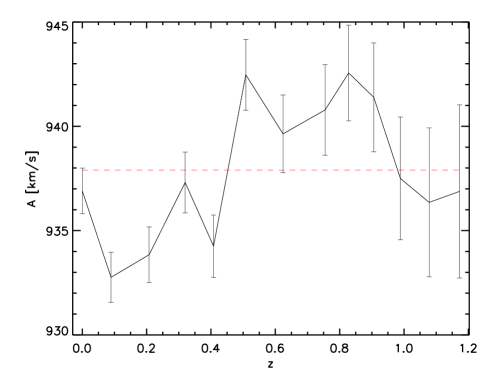
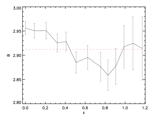
Figure 1.— The evolution of the normalization $A$ (left panel) and slope $B$ (right panel) parameters used to fit the relation between the 3D velocity dispersion of all the galaxies within $R_{\rm{vir}}$and the virial mass of each cluster (eq. 2). Red horizontal dashed lines represent the mean value. The slope is moderately shallower than the self-similar expectation.

2. Input Simulation

This analysis is based on the publicly available galaxy catalogue produced using the semi-analytic model (SAM) by De Lucia & Blaizot (2007) on the Millennium Simulation (Springel et al. 2005). The Millennium Simulation adopts the following values for the parameters of a flat $\Lambda$ cold dark matter model: $\Omega_{DM}=0.205$ and $\Omega_{b}=0.045$ for the densities in cold dark matter and baryons at redshift $z=0$, $\sigma_{8}=0.9$ for the rms linear mass fluctuation in a sphere of radius $8\mbox{$h^{-1}{\rm{Mpc}}~{}$}$, $h=0.73$ for the present dimensionless value of the Hubble constant and $n=1$ for the spectral index of the primordial fluctuation. The simulation follows the evolution of $2160^{3}$ dark matter particles from $z=127$ to the present day within a cubic box of $500\mbox{$h^{-1}{\rm{Mpc}}~{}$}$ on a side. The individual dark matter particle mass is $8.6\times 10^{8}h^{-1}\,{\rm M}_{\odot}$. The simulation was carried out with the massively parallel GADGET-2 code (Springel 2005). Gravitational forces were computed with the TreePM method, where long-range forces are calculated with a classical particle-mesh method while short-range forces are determined with a hierarchical tree approach (Barnes & Hut 1986). The gravitational force has a Plummer-equivalent comoving softening of $5\,h^{-1}{\rm kpc}$, which can be taken as the spatial resolution of the simulation. Full data are stored 64 times spaced approximately equally in the logarithm of the expansion factor. Dark matter halos and subhalos were identified with the friends-of-friends (FOF; Davis et al. 1985)) and SUBFIND (Springel et al. 2001a) algorithms, respectively. Based on the halos and subhalos within all the simulation outputs, detailed merger history trees were constructed, which form the basic input required by subsequently applied semi-analytic models of galaxy formation.

We recall that the SAM we employ builds upon the methodology originally introduced by Kauffmann et al. (1999), Springel et al. (2001b) and De Lucia et al. (2004b). We refer to the original papers for details.

The SAM adopted in this study includes explicitly DM substructures. This means that the halos within which galaxies form are still followed even when accreted onto larger systems. As explained in Springel et al. (2001) and De Lucia et al. (2004), the adoption of this particular scheme leads to the definition of different galaxy types. Each FOF group hosts a Central galaxy. This galaxy is located at the position of the most bound particle of the main halo, and it is the only galaxy fed by radiative cooling from the surrounding hot halo medium. Besides central galaxies, all galaxies attached to DM substructures are considered as satellite galaxies. These galaxies were previously central galaxies of a halo that merged to form the larger system in which they currently reside. The positions and velocities of these galaxies are followed by tracing the surviving core of the parent halo. The hot reservoir originally associated with the galaxy is assumed to be kinematically stripped at the time of accretion and is added to the hot component of the new main halo. Tidal truncation and stripping rapidly reduce the mass of DM substructures (but not the associated stellar mass) below the resolution limit of the simulation (De Lucia et al. 2004a; Gao et al. 2004). When this happens, we estimate a residual surviving time for the satellite galaxies using the classical dynamical friction formula, and we follow the positions and velocities of the galaxies by tracing the most bound particles of the destroyed substructures.

3. Properties of the Full Galaxy Population

3.1. Intrinsic galaxy velocity dispersion

Evrard et al. (2008) showed that massive dark matter halos adhere to a virial scaling relation when one expresses the velocity dispersion of the DM particles as a function of the virial mass of the halo in the form:

$$\sigma_{DM}(M_{vir},z)=\sigma_{DM,15}\left(\frac{h(z)M_{vir}}{10^{15}\,{\rm M}_{\odot}}\right)^{\alpha},$$ (1)

where $\sigma_{DM,15}=1082.9\pm 4.0\,{\rm km\,s^{-1}}$ is the typical 3D velocity dispersion of the DM particles within $R_{\rm{vir}}$ for a $10^{15}h^{-1}\,{\rm M}_{\odot}$ cluster at $z=0$ and $\alpha=0.3361\pm 0.0026$. Similarly, we first compute for each cluster the 3D velocity dispersion $\sigma_{3D}$ (divided by $\sqrt{3}$) of all the galaxies within $R_{\rm{vir}}$and then fit the relation between $\sigma_{3D}$ and $M_{\rm{vir}}$ in the form of $log(\sigma_{3D})\propto log(h_{70}(z)\mbox{$M_{\rm{vir}}$ }/10^{15}\,{\rm M}_{\odot})$ individually at any of the redshift listed in Table 1. As a result we can express the dynamical mass $M_{dyn}$ as:

$$M_{dyn}=\left(\frac{\sigma_{v}}{A}\right)^{B}h_{70}(z)^{-1}10^{15}\,{\rm M}_{\odot},$$ (2)

where the resulting best fitting values of A and B with their associated error-bars are shown in Fig. 1 as a function of redshift. Dashed horizontal red lines show the average values which are respectively $\bar{A}=938\pm 3\,{\rm km\,s^{-1}}$ and $\bar{B}=2.91\pm 0.03$.

After accounting for the differences in the Hubble parameter, our measured normalization of the galaxy velocity dispersion– mass relation is within $\lesssim$3% of Evrard et al. (2008). This reflects the differences between the subhalo and DM particle dynamics. As has been previously pointed out (e.g. Gao et al. 2004, Goto 2005,Faltenbacher & Diemand 2006, Evrard et al. 2008, White et al. 2010), the velocity bias between galaxies and DM is expected to be small $b_{v}\lesssim 5\%$. But to be absolutely clear, we adopt our measured galaxy velocity dispersion– mass calibration in the analyses that follow. To better visualize the relative importance of the cosmological redshift dependence we show in Fig. 2 the redshift evolution of the normalisation parameter $A$ (solid black line )when the fit is made on the relation $log(\sigma_{3D})\propto log(h_{70}(z=0)\mbox{$M_{\rm{vir}}$ }/10^{15}\,{\rm M}_{\odot})$. The expected self-similar evolution given by $A(z)=\bar{A}\times E(z)^{1\over 3}$ is highlighted (dashed red line), where the term $\bar{A}$ is equal to mean value $\bar{A}=938\,{\rm km\,s^{-1}}$ and $E(z)$ describes the universal expansion history $H(z)=H_{0}E(z)$. In other words, Fig. 2 shows the typical galaxy velocity dispersion in $\,{\rm km\,s^{-1}}$ for a cluster with $M_{\rm{vir}}$ $=10^{15}\,h_{70}^{-1}{\rm M}_{\odot}$ as a function of redshift and demonstrates the nearly self-similar evolution (within $\sim$1%) over the redshift range tested in this work.

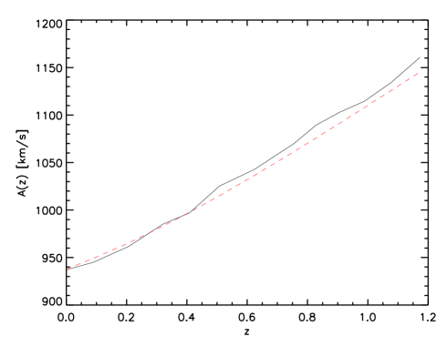
Figure 2.— The evolution of the normalisation parameter $A(z)$ of Eq. 2 when no self-similar evolution is taken into account (solid black line). Red dashed line is showing the best fitting parameter $\bar{A}\times\left(H(z)/H_{0}\right)^{1\over 3}$

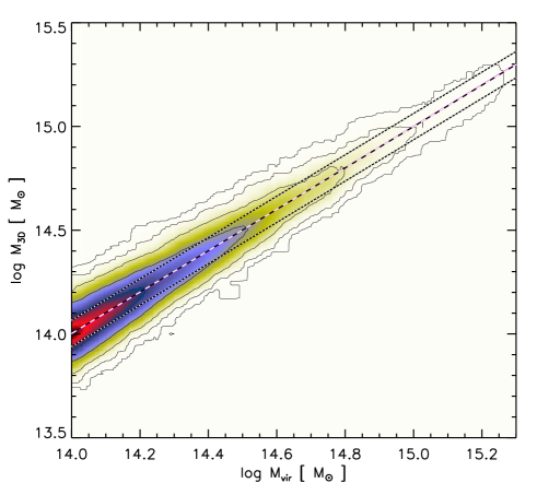
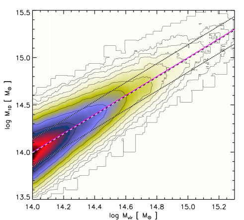
Figure 3.— The relation between $M_{\rm{vir}}$ and the dynamical mass for all the clusters in the sample. For each cluster the dynamical mass is inferred by applying Eq. 2 to the 3D velocity dispersion divided by $\sqrt{3}$ (left panel) and for each of the three projected 1D velocity dispersions (right panel) of all the galaxies extracted from the De Lucia & Blaizot (2007) database within $R_{\rm{vir}}$ from the centre of the cluster. The dashed (dotted) white-black line is the best fit of the relation (plus and minus one $\sigma$) and is virtually indistinguishable from the one-to-one relation (dotted-dashed purple line).

For the full sample of clusters analysed (see Table 1), we then compute the dynamical masses by applying Eq. 2 to (1) the 3D galaxy velocity dispersion (divided by $\sqrt{3}$) and (2) to each orthogonal projected 1D velocity dispersion. Fig. 3 shows the comparison between the virial masses $M_{\rm{vir}}$ and the resulting dynamical masses $M_{3D}$ (left panel) and $M_{1D}$ (right panel) for the full sample of clusters. The best fit of the relation (dashed black and white lines) is virtually indistinguishable from the one-to-one relation (dotted-dashed purple line) in the case of the 3D velocity dispersion. On the other hand, in the case of the 1D velocity dispersion there is a small but detectable difference between the one-to-one relation and the best fit. The best fit of the dynamical mass for the 1D velocity dispersion is about $\lesssim 1\%$ lower than the one-to-one relation. We will show in Section 3.2 that this difference can be explained in terms of triaxial properties of halos. Typical logarithmic scatter of $\sigma_{M_{3D}/M_{vir}}\simeq 0.145$ and $\sigma_{M_{1D}/M_{vir}}\simeq 0.334$ are highlighted with dotted black and white lines in $log_{10}$ scale. We find that, similar to results by White et al. (2010), using the 1D velocity dispersion rather than the 3D velocity dispersion increases the intrinsic log scatter around the mean relation by a factor of $\sim 2.3$.

We further investigate the intrinsic scatter in the relation between the true virial masses and the dynamical mass estimates in Fig. 4. Taking $\sigma$ to be the standard deviation of the logarithm of the ratio between the dynamical mass estimate and the virial masses, we show that in the case of the 3D velocity dispersion (dashed red line) and the 1D velocity dispersion (dotted black line) the scatter increases with redshift. The solid black line shows a linear fit to the evolution of the intrinsic $M_{dyn-1D}$ scatter and can be expressed as:

$$\sigma_{ln(M_{1D}/M_{vir})}\simeq 0.3+0.075\times z.$$ (3)

Velocity dispersions are $\sim$25% less accurate for estimating single cluster masses at $z=1$ than at low redshift.

The logarithmic scatter of the 1D velocity dispersion mass estimator $\sigma_{M_{1D}}$ around the true mass arises from two sources of scatter: (1) the logarithmic scatter between the 3D velocity dispersion mass estimator and the true mass - $\sigma[M_{3D}/M_{vir}]$ (red dashed line in Fig 4) and (2) the logarithmic scatter between the 1D and 3D velocity dispersions $\sigma[\sigma_{1D}/\sigma_{3D}]$ (solid green line). The expected 1D dispersion mass scatter is then the quadrature addition of these two sources:

$$\sigma^{2}_{M_{1D}}\sim\sigma^{2}[M_{3D}/M_{vir}]+\{\bar{B}\times\sigma[\sigma_{1D}/\sigma_{3D}]\}^{2},$$ (4)

where $\bar{B}$ is the best fitting slope parameter from Eq. 2. The expected $\sigma_{M_{1D}}$ estimate from Eqn. 4 appears as a dotted-dashed purple line in Fig 4; note that this estimate is in excellent agreement with the directly measured scatter (dotted black line). Therefore, we show– as pointed out by White et al. (2010)– that the dominant contributor to the scatter is the intrinsic triaxial structure of halos. Furthermore its evolution with redshift is also the dominant source of the increasing scatter of the 1D dynamical mass estimates with redshift. By comparison, the scatter between the 3D velocity dispersion mass estimator and the true mass $\sigma[ln(M_{3D}/M_{vir})]$, which is reflecting departures from dynamical equilibrium due to ongoing merging in the cluster population, is relatively minor. Ultimately it is the lack of observational access to the full 3D dynamics and distribution of the galaxies that limits us from precise single cluster dynamical mass estimates.

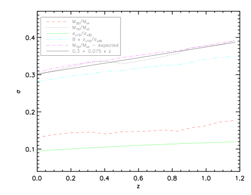
Figure 4.— The redshift evolution of the logarithmic 1$\sigma$ scatter for the following quantities: (1) the 3D galaxy velocity dispersion mass estimate scatter (dashed red), (2) the 1D galaxy velocity dispersion mass estimate scatter (dotted black), (3) a fit to #2 (solid black; Eqn. 3), (4) the scatter of the 1D velocity dispersion about the 3D dispersion (solid green), (5) the same quantity turned into mass scatter using Eqn. 2 (dashed-dotted blue) and (6) the expected 1D dispersion mass scatter (#2) obtained by quadrature addition of #1 and #5, as explained in Sec. 3.1 (dotted-dashed purple; Eqn. 4).

3.2. Triaxiality

The presence of pronounced departures from sphericity in dark matter halos (Thomas & Couchman 1992, Warren et al. 1992, Jing & Suto 2002), if not approximately balanced between prolate and oblate systems, could in principle not only increase the scatter in dynamical mass estimates, but also lead to a bias. If, for example, clusters were mainly prolate systems, with one major axis associated to a higher velocity dispersion and two minor axes with a lower velocity dispersion, there should be two lines of sight over three associated with a lower velocity dispersion. This could potentially lead to a bias in the 1D velocity dispersion with respect to the 3D velocity dispersion. To quantify this possible bias, we compute the moment of inertia for each cluster in the sample, and we then calculate the velocity dispersions along each of the three major axes. As has been pointed out before (Tormen 1997, Kasun & Evrard 2005, White et al. 2010) the inertia and velocity tensor are quite well aligned, with typical misalignment angle of less than $30^{\circ}$. In Fig. 5, at each redshift we show the lowest velocity dispersion $\sigma_{0}$ with black crosses, the highest $\sigma_{2}$ with green stars and the intermediate one $\sigma_{1}$ with red diamonds normalized to the 3D velocity dispersion $\sigma_{3D}$ (divided by $\sqrt{3}$). Dashed blue lines are the 16, 50 and 84 percentile of the full distribution and DEV is the associated standard deviation which, as expected from Fig. 4 is increasing with redshift. A perfectly spherical cluster in this plot will therefore appear with the three points lying all at the value 1, whereas prolate and oblate systems will have the intermediate velocity dispersions $\sigma_{1}$ closer to the lower one $\sigma_{0}$ and to the higher one $\sigma_{2}$, respectively. The black solid line is the best fit of the distribution of the intermediate $\sigma_{1}$ velocity dispersions and it is very close to unity, showing that dynamically, clusters do not have a very strong preference among prolate and oblate systems. Furthermore this result is true for the range of redshifts and masses we examine here.

This can be better seen in Fig. 6, where we show that we measure only a mild excess (at $\lesssim 5\%$ level) of prolate systems. In addition, for each cluster in the sample, we compute a ”prolateness” quantity $Prol$ as:

$$Prol=\frac{\left(\sigma_{2}-\sigma_{1}\right)-\left(\sigma_{1}-\sigma_{0}\right)}{\sigma_{3D}}.$$ (5)

A prolate system will have a positive $Prol$ value whereas an oblate one will have a negative $Prol$. Fig. 6 shows a map representing the distribution of the $Prol$ variable as a function of the cluster mass (left panel) and redshift (right panel). To compute the former we stack clusters from all the redshifts, and for the latter we stack clusters from all masses. As it is shown in Fig. 6, there are no clear dependencies of the $Prol$ variable on the cluster mass or redshift. The slight excess of prolate over oblate systems at all masses and redshifts would translate into 1D dynamical masses slightly biased towards smaller masses. Indeed, this is seen as a $\sim 1$% effect in Fig. 3.

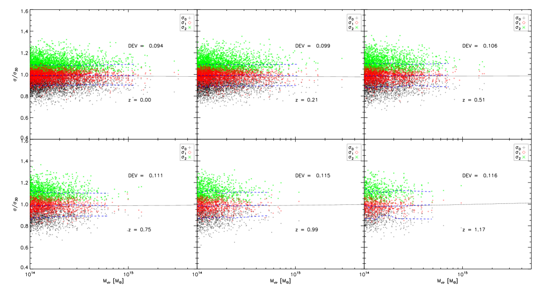
Figure 5.— We show for each cluster the velocity dispersion along the tree major axes of the inertia momentum (black crosses for the smaller, red diamonds for the intermediate and green stars for the larger) normalized to the 3D velocity dispersion divided by $\sqrt{3}$ as a function of the cluster mass in different redshift bins. The black solid line is the best fit of the intermediate axis velocity dispersion, and the dashed blue lines are the median and the 16 and 84 percentile of the full distribution. DEV is the associated standard deviation.

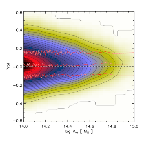
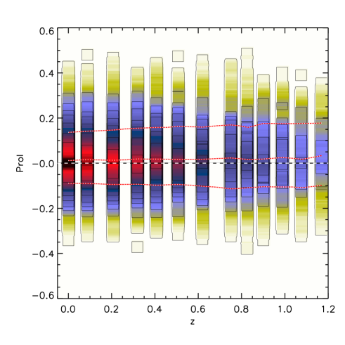
Figure 6.— The distribution of the prolateness variable $Prol$ (see Eqn. 5) as a function of the cluster mass for all the clusters at different redshift stacked together (left panel) and as a function of redshift (right panel). To guide the eye the dashed black and white line is highlighting the value of $Prol=0$, while the dotted red-white lines are respectively the 16, 50 and 84 percentiles for the two different distributions. The cluster ensemble exhibits a slight preference for prolateness at all masses and redshifts.

4. Properties of Spectroscopic Subsamples

Results in the previous section relied on the full galaxy sample within each cluster virial region. We now study the possible systematics affecting the cluster velocity dispersion and associated dynamical mass estimates when more realistic selection for the member galaxies are taken into account.

We model the selection carried out in real world circumstances by following the procedure we have developed for the South Pole Telescope (SPT) dynamical mass calibration program (Bazin et al. 2012). Namely, we preferentially choose the most luminous red sequence galaxies that lie projected near the center of the cluster for our spectroscopic sample. To do this we select galaxies according to their colors, which are a direct prediction of the adopted semi-analytic model. In particular, we compute the following color-magnitude diagrams for different redshift ranges: $g-r$ as a function of $r$ for redshift z$\leq 0.35$, $r-i$ as a function of $i$ for redshifts $0.35<$z$\leq 0.75$ and $i-z$ as a function of $z$ for redshifts larger than 0.75 (e.g. Song et al. 2011). We report in Fig. 7 the color-magnitude diagram at different redshifts for all the galaxies within the virial radius of each cluster. The model given by Song et al. (2011), which has proven to be a good fit to the observational data, is highlighted with a dashed black-red line. As it is shown, the simulated cluster galaxy population has a red-sequence flatter than the observational results. Because the purpose of this work is not to study the evolution of the cluster galaxy population, but rather to see the effect of the selection of galaxies on the estimated dynamical mass, we adopt the following procedure: First we fit the red sequence at each analysed redshift. Then, we symmetrically increase the area on color-magnitude space in order to encompass $68\%$ of the galaxies and iterate the fit. The resulting best fit and corresponding area are highlighted as green continuous and dashed lines in Fig. 7. Table 2 describes the width in color space used to select red sequence galaxies at each analysed redshift.

Table 2Color width of the simulated red sequence in magnitudes at each analysed redshift. Column 1: redshift; Column 2: 1 $\sigma$ width of the red sequence in magnitudes.

z	mag
0.00	0.05
0.09	0.06
0.21	0.08
0.32	0.10
0.41	0.06
0.51	0.08
0.62	0.08
0.75	0.08
0.83	0.09
0.91	0.09
0.99	0.07
1.08	0.06
1.17	0.05

This color selection helps to reduce the interlopers in our cluster spectroscopic sample. In addition to color selection, we explore the impact of imposing a maximum projected separation $R_{\perp}$ from the cluster center, and we explore varying the spectroscopic sample size. In all cases we use the $N_{gal}$ most massive (and therefore luminous) galaxies in our selected sample. Table 3 shows the range of $N_{gal}$ and $a=R_{\perp}/r_{vir}$ that we explore as well as the sample binning in redshift and mass. Note that for SZE selected clusters from SPT or equivalently X-ray selected samples of clusters, once one has the cluster photometric redshift one also has an estimate of the cluster virial mass and virial radius from SZE signature or X-ray luminosity (e.g. Reiprich & Böhringer 2002, Andersson et al. 2011); therefore, we do in fact restrict our spectroscopic sample when building masks according to projected distance from the cluster center relative to the cluster virial radius estimate.

Table 3Parameter space explored for the mock observations. Column 1: maximum projected distance $R_{\perp}$ from cluster center $a=R_{\perp}/r_{vir}]$; Column 2: $N_{gal}$ initial number of selected most massive red-sequence galaxies; Column 3: redshift $z$; Column 4: cluster mass $M_{\rm{vir}}$ [$10^{14}\,{\rm M}_{\odot}$].

$a$	$N_{gal}$	z	$M_{\rm{vir}}$
0.2	10	0.00	1.0
0.4	15	0.09	2.0
0.6	20	0.21	4.0
0.8	25	0.32	6.0
1.0	30	0.41	8.0
1.2	40	0.51	10.0
1.4	50	0.62	20.0
1.6	60	0.75
1.8	75	0.83
2.0	100	0.91
2.2		0.99
2.4		1.08
		1.17

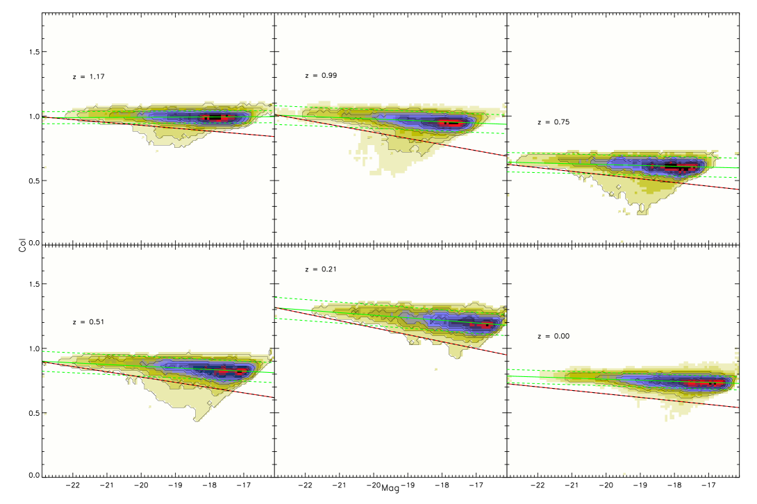
Figure 7.— Color magnitude relation for all the galaxies within $R_{\rm{vir}}$at six different redshifts. Color-magnitude relations are expressed as $g-r$ as a function of $g$ for redshift z$\leq 0.35$, $r-i$ as a function of $i$ for redshifts $0.35<$z$\leq 0.75$ and as $i-z$ as a function of $z$ for redshifts larger than 0.75 (see text for further details). Symbols with different colors refers to different galaxy clusters in each separate redshift bin. Dashed black-red line is the model given by Song et al. (2011). The solid green lines are the best fit to the simulated red-sequence relation used in this work and dashed green lines enclose $68\%$ of the galaxies. The area between them represents the color space used for the selection of galaxies described in Sect. 4.

4.1. Dynamical friction and Velocity Bias

In section 3.1 we showed the presence of a tight relation between the 3D dynamical mass and the virial mass $M_{\rm{vir}}$  for galaxy clusters. When dynamical masses are computed from the 1D velocity dispersion instead of the 3D one, we significantly increase the scatter of this relation and introduce a negligible bias ($\lesssim 1\%$) due to the triaxial properties of dark matter halos. We now study the effect of velocity segregation due to dynamical friction and its effect on the estimated dynamical masses. To do this, for each cluster we select a number of red-sequence galaxies within the virial radius $R_{\rm{vir}}$that ranges from 10 to 100 galaxies as described in Table 3. We sort galaxies according to their luminosity (different bands were used at different redshift as described in Sec. 4). This results in a ”cumulative” selection. Therefore, for example, for each cluster the 10 most luminous red-sequence galaxies are present in all the other samples with larger number of galaxies. On the other hand, when a cluster field is spectroscopically observed, completeness to a given limiting magnitude is not always achieved. In fact, the number of slits per mask in multi-slit spectrographs is fixed, hence the central, high-density regions of galaxy clusters can often be sampled only to brighter magnitudes than the external regions. As a consequence, the spatial distribution of the galaxies selected for spectroscopy turns out to be more extended than the parent spatial distribution of cluster galaxies. In the analyses presented here, we do not model this observational limitation. Indeed, as described in the companion paper Bazin et al. (2012), such difficulty could be easily overcome by applying multiple masks to the same field, which would allow one to achieve high completeness. For each cluster and for all the three orthogonal projections, we then compute the robust estimation of the velocity dispersion Beers et al. (1990) with different numbers of galaxies and compare it with the intrinsic 1D velocity dispersion. Fig. 8 shows the probability distribution function (PDF) of the ratio between the velocity dispersion computed with different numbers of bright red-sequence cluster galaxies ($\sigma_{Ngal}$) and the intrinsic 1D velocity dispersion ($\sigma_{1D}$) obtained by stacking results from all the lines of sight of the cluster sample. Different colors refer to different numbers of galaxies and the mean of each distribution is highlighted at the top of the plot with a vertical line segment. We note that when large numbers of galaxies are used to estimate the velocity dispersion, the probability distribution function is well represented by a log-normal distribution centered at zero. As a result dynamical masses obtained from large numbers of bright red-sequence cluster galaxies are unbiased with respect to the intrinsic 1D dynamical mass. However, when the number of red-sequence galaxies used to estimate the velocity dispersion is lower than $\sim 30$, the corresponding PDF starts to deviate from a symmetric distribution and its mean is biased towards lower values. This effect is evidence of a dynamically cold population of luminous red galaxies whose velocities are significantly slowed due to dynamical friction processes. Indeed dynamical friction is more efficient for more massive galaxies, hence the velocity bias is expected to be more important for the bright end of the galaxy population (e.g. Biviano et al. 1992, Adami et al. 1998, Cappi et al. 2003, Goto 2005, Biviano et al. 2006).

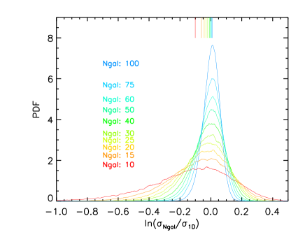
Figure 8.— The probability distribution function of the measured velocity dispersion computed with different numbers of red-sequence cluster galaxies sorted by luminosity and normalized by the intrinsic 1D velocity dispersion using the full galaxy sample. The position of the mean of each curve is highlighted with a vertical line segment at the top of the figure. Small samples of the most luminous galaxies exhibit biases in dispersion and significant asymmetries in the PDF.

To verify this we compute $\sigma_{Ngal}$ in the same way described above, but starting from galaxies that are randomly selected with respect to luminosity. Note that in this case we only randomly select galaxies, but we don’t change the ”cumulative nature” of our selection and the subsequent estimated velocity dispersion when using larger numbers of galaxies. We then calculate the corresponding dynamical masses in the case of galaxies selected according to the procedure described in Sect. 4 and in the case of random selection using the different number of galaxies listed in Table 3. The resulting stacked dynamical masses for the full sample of clusters and for the three orthogonal projections are shown in Fig. 9 as a function of the intrinsic virial mass $M_{\rm{vir}}$ . The dashed purple-black line is the one-to-one relation and the solid green lines are the median and 16 and 84 percentiles of the distributions. The left panel of Fig. 9 represents the original distribution, while the right panel represents the randomly selected distribution. As expected from Fig. 8, if velocity dispersions are computed from red-sequence galaxies selected according to their luminosity, a clear bias is introduced in the estimated dynamical mass. Moreover we can see that the distance between the median line and the 84 percentile line is smaller than the distance between the median and the 16 percentile line, because the distribution is no longer symmetric.

Furthermore it appears that the bias present in the estimated dynamical mass does not depend on the cluster mass. On the other hand, if we randomly select galaxies (right panel), the bias is reduced, and we obtain a more symmetric distribution. We also check for a possible redshift dependency on the velocity bias or dynamical friction. For this purpose we split our sample of clusters into two different redshift bins and show separately in Fig. 10 the relation between the true cluster virial mass and the estimated dynamical masses computed with different number of bright red-sequence galaxies selected according to their luminosity in the case of low redshift (left panel) and high redshift (right panel) clusters. Obviously the number of clusters and their mass distribution is a strong function of redshift. However, it is worth noting that the impact of dynamical friction on the estimation of velocity dispersion and dynamical mass does not vary much with cluster mass or redshift.

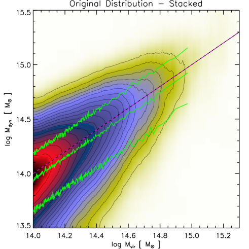
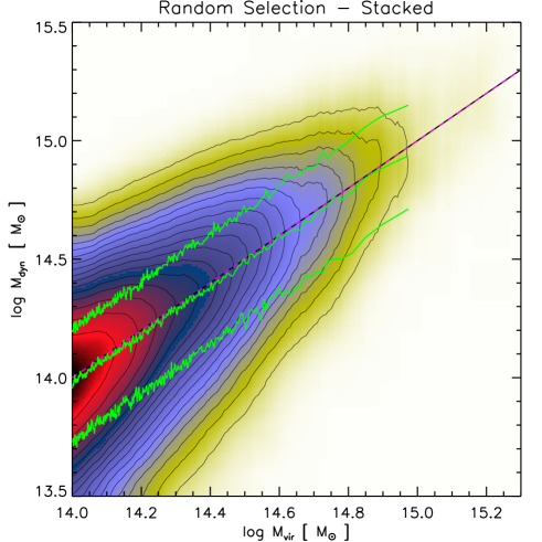
Figure 9.— The relation between $M_{\rm{vir}}$ and the dynamical mass for all the clusters in the sample and for each orthogonal projection. For each cluster the dynamical mass is infer-ed by applying Eq. 2 to the robust estimation of the velocity dispersion computed using different number of galaxies (Table 3). Left panel is for bright red-sequence galaxies sorted according to their luminosity and right panel is for a randomly sorted array of galaxies. Dashed purple-black line is the one-to-one relation, and solid green lines represent the 16, 50 and 84 percentiles.

Using the results of these mock observations we express both the velocity dispersion bias, represented by the position of the vertical segment at the top of Fig. 8, and the characteristic width of each distribution shown in Fig. 8 with the following parametrisation:

$$<ln(\sigma_{Ngal}/\sigma_{1D})>=0.05-0.51/\sqrt{Ngal},$$ (6)

$$\sigma_{ln(\sigma_{Ngal}/\sigma_{1D})}=-0.037+1.047/\sqrt{Ngal}.$$ (7)

This parametrisation is valid only in the limit of the number of galaxies used in this study (between 10 and 100). For example if the dynamical mass is estimated starting from a number of galaxies larger than 100, the bias would presumably be zero rather than negative as implied from Eq. 6.

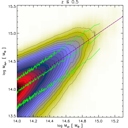
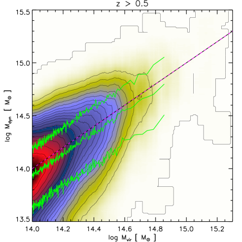
Figure 10.— Same as for the left panel of Fig. 9, but dividing our cluster sample in 2 redshift bins. Left panel is for $z\leq 0.5$ and right panel is for $z>0.5$.

We demonstrate in Fig. 11 that by applying Eq. 6 to the velocity dispersion estimated with different numbers of red-sequence cluster galaxies we are able to remove the bias induced by the dynamical friction. In particular, Fig. 11 shows the relation between true virial mass and the dynamical mass estimated using the most luminous 100, 50 and 15 red-sequence galaxies. Dynamical masses are computed by applying Eq. 2 directly to the velocity dispersion (left panels) and to the velocity dispersion corrected according to Eq. 6 (right panels). Dynamical friction is affecting mostly the bright end of the red-sequence cluster galaxies population and therefore the bias is larger in the case of the smallest sample (lower left panel). Consistently the correction given by Eq. 6 is larger in this case, whereas it is negligible in the other cases (50 and 100).

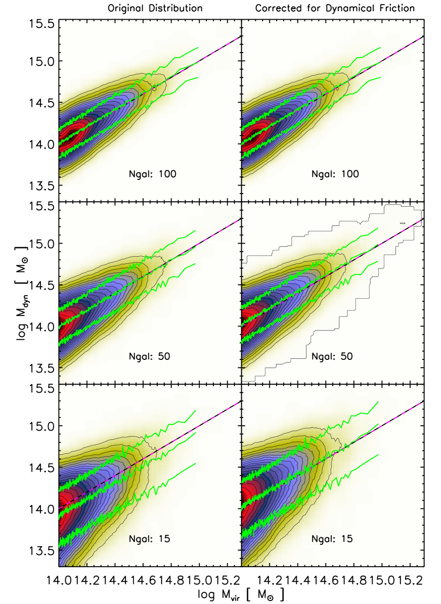
Figure 11.— The relation between $M_{\rm{vir}}$ and the dynamical mass for all the clusters in the sample and for each orthogonal projection. Left panels: For each cluster the dynamical mass is infer-ed by applying Eq. 2 to the robust estimation of the velocity dispersion computed using the 100, 50 and 15 most luminous red-sequence cluster galaxies (with distance from the centre smaller than $R_{\rm{vir}}$) and show respectively in the upper, middle and lower panels. Right panels: Same as for left panels, but velocity dispersions are corrected according to Eq. 6. Dashed purple-black line is the one-to-one relation, and solid green lines represent the 84, 50 and 16 percentiles.

4.2. Impact of Poisson Noise

In this work we restrict our analyses to all the galaxies with stellar masses predicted by the adopted SAM larger than $5\times 10^{8}\,{\rm M}_{\odot}$. The total number of galaxies within the virial radius $R_{\rm{vir}}$ is therefore quite large and even for the poorer clusters with $\mbox{$M_{\rm{vir}}$ }\sim 10^{14}\,{\rm M}_{\odot}$, the number of galaxies used to compute the 1D velocity dispersion is of the order of $N_{1D}\sim 200$. As a result, in the absence of any dynamical friction effect, the associated characteristic scatter to the ratio $\sigma_{Ngal}/\sigma_{1D}$ is well represented by the Poissonian factor $\sqrt{2N_{gal}}$. To demonstrate it, we show in Fig. 12 the evolution of the scatter in the relation between the true virial masses and the dynamical masses as a function of redshift. For each cluster, dynamical mass is estimated starting from the velocity dispersion of the 100 most luminous red-sequence galaxies through Eq. 2. The resulting scatter is highlighted as a cyan solid line. We also show the evolution of associated scatter when dynamical mass is computed from the intrinsic 3D (dashed red line) and 1D (dotted black line) velocity dispersions. Moreover, similarly to Fig. 4, we separately show the predicted scatter obtained by adding in quadrature the scatter associated to the 1D velocity dispersion with the Poisson term $\sqrt{2N_{gal}}$ (dashed-triple dotted green line) or with the factor given by Eq. 7 (dashed-dotted purple line). We note that, as expected, both predictions agree very well with the measured evolution of the scatter.

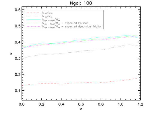
Figure 12.— The evolution of the 1 $\sigma$ scatter as a function of redshift in log-space for the following quantities. Dashed red (dotted black) line is for the ratio between the estimated dynamical mass $M_{3D}$ ($M_{1D}$) computed from the 3D (1D) velocity dispersion and the virial mass $M_{\rm{vir}}$ . The solid cyan line is for the ratio between the measured dynamical mass $M_{dyn}$ computed from the 100 most luminous red-sequence galaxies within the virial radius of each cluster along each line of sight and the virial mass $M_{\rm{vir}}$ . The dashed-dotted green line is the expected scatter in mass obtained by multiplying $B$ by the term given by adding in quadrature the scatter from the 1D velocity dispersion and a Poissonian term equal to $\sqrt{2\times 100}$. The dashed-dotted purple line is the expected scatter in mass obtained by multiplying $B$ by the term given by adding in quadrature the scatter from the 1D velocity dispersion and a term computed with the fitting formula of Eq. 7.

However, if a lower number of galaxies is used to calculate the dynamical mass, a difference in the two predictions emerge. For example, in Fig. 13 we show the same computation highlighted in Fig. 12, but with a number of galaxies equal to 50 (left panel) and 15 (right panel). We note in particular that the observed evolution of the scatter of the relation among the virial mass and the dynamical mass is well described by adding in quadrature to scatter associated to the intrinsic 1D dynamical mass the term given by the fitting formula of Eq. 7. On the contrary, if only the Poisson term $\sqrt{2N_{gal}}$ is taken into account, the predicted scatter is underestimated with respect to the measured one. Furthermore, note that while on the one hand in Figures 11 and 8 we showed that the dispersion calculated using 50 galaxies does not introduce a significant mass bias; however, it is clear that the Poisson term is no longer adequate to explain the real scatter. On the other hand, if the contribution to the scatter due to dynamical friction is included through Eq. 7 we are able to recover the right answer.

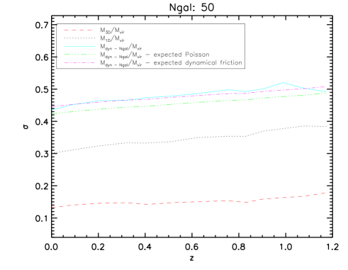
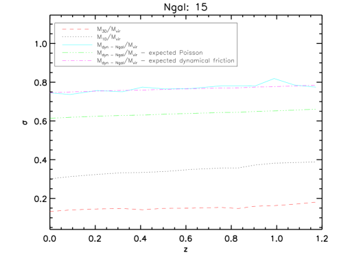
Figure 13.— Same as for Fig. 12, but with a number of galaxies respectively equal to 50 (left panel) and 15 (right panel).

4.3. Impact of Interlopers

Finally, to have a more coherent and realistic approach to our analyses, we further investigate the effect of interlopers as a possible source of systematics in the computation of clusters dynamical mass. For this purpose, for each snapshot and projection, we construct a number of cylindrical light-cones centred at each cluster with height equal to the full simulated box-length and different radius spanning the interval 0.2 to 2.4 $R_{\rm{vir}}$. The different aperture values used are listed in Table 3. We then apply an initial cut of $4000\,{\rm km\,s^{-1}}$ to select galaxies within the cylinders. For each cylindrical light-cone realisation, we then initially select a different number of members in the color-magnitude space described in Sect. 4 ranging from 10 to 100 galaxies as shown in Table 3. Several techniques have been developed to identify and reject interlopers. Such methods have been studied before typically using randomly selected dark matter particles (e.g. Perea et al., 1990; Diaferio & Geller, 1997; Łokas et al., 2006; Wojtak et al., 2007, 2009) and more recently using subhalos by Biviano et al. (2006) and White et al. (2010). However, for the purpose of this work, here we simply apply a 3$\sigma$ clipping procedure to its robust estimation of the velocity dispersion Beers et al. (1990) to reject interlopers, as discussed in Bazin et al. (2012). This leads to a final spectroscopic sample of galaxies for each cluster, at each redshift, for each projection, within each different aperture and for each different initially selected number of red-sequence galaxies. Fig. 14 is a schematic representation of the procedure we follow to obtain from each cluster and projection different estimation of the velocity dispersion according to different ”observational choices”.

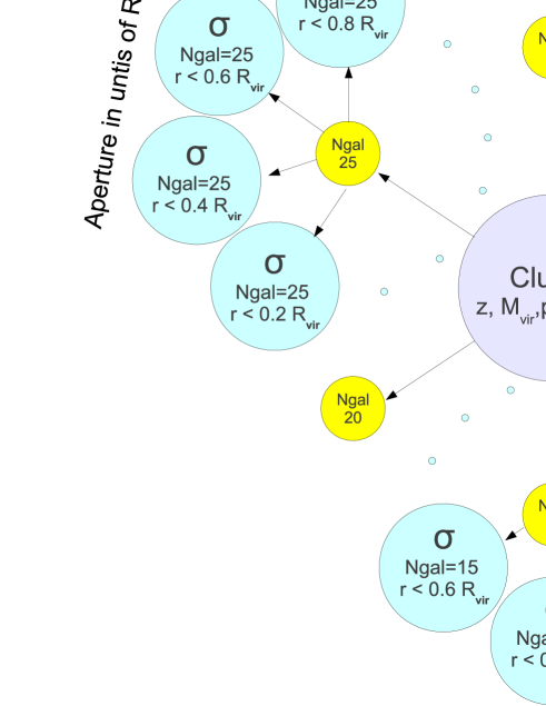
Figure 14.— Schematic representation of the parameter space explored in this work. See Table 3 for specific ranges in each parameter.

From final spectroscopic sample of galaxies described above, we compute the fraction of interlopers (arbitrary defined here as galaxies lying at a cluster centric distance larger than 3$\times$$R_{\rm{vir}}$) as a function of the aperture by stacking together the sample in different bins according to their redshift, to the number of galaxies used to evaluate their velocity dispersion and to the cluster masses. This can be seen in Figure 15 and is in good agreement with previous works (e.g. Mamon et al. 2010). The two upper panels and the lower-left panel show the fraction of interlopers as a function of aperture respectively color coded according to the number of galaxies (panel A), to the redshift (panel B) and to the cluster mass (panel C). As expected, the fraction of interlopers rises with the aperture within which the simulated red-sequence galaxies were initially chosen. This indicates that even red sequence, spectroscopically selected samples are significantly contaminated by galaxies lying at distances more than three times the virial radius from the cluster.

On the other hand a much weaker dependency between the number of selected red sequence galaxies and the fraction of interlopers is highlighted on the upper-left panel of Fig. 15 (A). Whether one has small or large samples the fraction of interlopers remains almost the same. The upper-right and the bottom-left panels are showing that the fraction of interlopers is larger at larger redshifts consistently with a denser Universe (B), and is a steeper function of aperture for lower mass clusters (C). Since in the hierarchical scenario more massive halos forms at later times than the lower mass ones, these two variables are clearly correlated. Thus, we also show in the bottom-right panel labeled ”D” how the fraction of interlopers varies as a function of redshift by stacking together the sample in different mass bins. Most massive clusters are not formed yet at high redshifts, therefore above certain redshifts the redder lines go to zero. Although oscillating, an evident tendency of increasing fraction of interlopers is associated to larger redshift, whereas at fixed $z$ there is no clear dependency of the fraction of interlopers from the clusters mass. We stress however that all the relations shown in Fig. 15 are meant to describe the qualitative dependency of the interloper fraction from the analysed quantities.

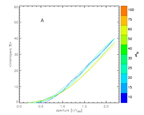
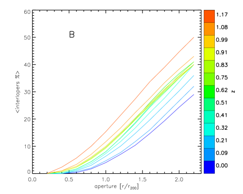
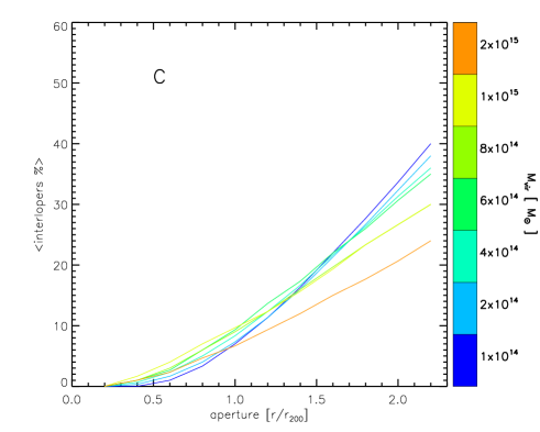
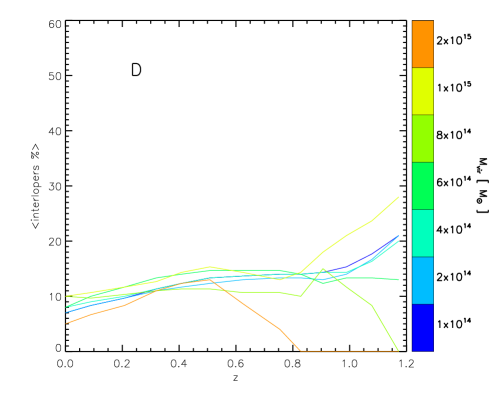
Figure 15.— Upper panels and bottom left panel: The stacked mean fraction of interlopers (defined as galaxies at distance larger than $3\times$ $R_{\rm{vir}}$) as a function of maximum projected separation from the cluster $R_{\perp}$ normalized to $R_{\rm{vir}}$ color coded in numbers of galaxies used to estimate the velocity dispersion (top left panel labeled A), redshift (top right panel labeled B) and mass of the cluster (bottom left panel labeled C). Bottom right panel: The stacked mean fraction of interlopers as a function of redshift color coded according to the cluster mass (labeled D).

In a similar way we compute the mean velocity bias (defined as the ratio between the measured velocity dispersion and the intrinsic line-of-sight velocity dispersion: $\sigma_{(N_{gal},R_{\perp},M_{vir},z)}/\sigma_{1D}$) as a function of the aperture by stacking together the sample in different bins according to their redshift, to the number of spectroscopic galaxies and to the cluster mass. This can be seen in Figure 16. The two upper panels and the lower-left panel show the velocity bias as a function of aperture respectively color coded according to the number of galaxies (panel A), to the redshift (panel B) and to the cluster mass (panel C). Interestingly, the velocity bias has a minimum when velocity dispersions are evaluated within $R_{\perp}\sim\mbox{$R_{\rm{vir}}$}$, and rises at both smaller and larger radii. In particular, for projected radii $\lesssim\mbox{$R_{\rm{vir}}$}$, where the effect of interlopers is smaller, we recover the expected decrease of the average velocity dispersion profile (e.g. Biviano et al. 2006) as a function of aperture. On the other hand, for $R_{\perp}\gtrsim\mbox{$R_{\rm{vir}}$}$, the larger contamination from interlopers is significantly affecting and boosting the velocity bias. Furthermore, as expected, dynamical friction is also affecting the estimated velocity dispersion, when the latest is computed with a small number of selected red sequence galaxies (A). Indeed, by applying Eq. 6 to the estimated velocity dispersion we are able to successfully remove the degeneracy between the velocity bias and the number of galaxies within projected aperture $R_{\perp}\lesssim\mbox{$R_{\rm{vir}}$}$ (Fig. 17). The upper-right and the bottom-left panels of Fig. 16 show that, consistent with the fraction of interlopers, the velocity bias computed within $R_{\perp}\gtrsim\mbox{$R_{\rm{vir}}$}$ is larger at larger redshifts (B) and is a steeper function of aperture for lower mass clusters (C). Finally, a mild dependence of redshift for fixed mass is highlighted in the bottom-right panel (D).

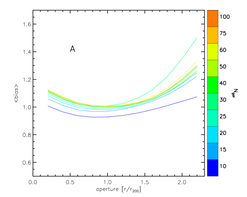
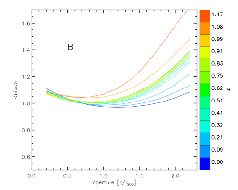
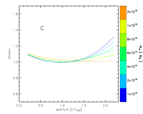
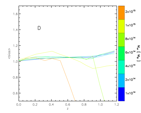
Figure 16.— Upper panels and bottom left panel: The stacked mean velocity bias as a function of maximum projected separation from the cluster $R_{\perp}$ normalized to $R_{\rm{vir}}$ color coded in numbers of galaxies used to estimate the velocity dispersion (top left panel labeled A), redshift (top right panel labeled B) and mass of the cluster (bottom left panel labeled C). Bottom right panel: The stacked mean velocity bias as a function of redshift color coded according to the cluster mass (labeled D).

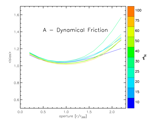
Figure 17.— Upper panels and bottom left panel: Same as Fig. 16 - panel A, but corrected for dynamical friction according to Eq. 6.

To better understand how interlopers affect the inferred velocity dispersion we select as an example all clusters with $M_{\rm{vir}}$  larger than $5\times 10^{14}\,{\rm M}_{\odot}$. For each of the three orthogonal projections we then initially select the most luminous 25 red-sequence galaxies as described in Sect. 4 within a projected distance of $1.5\mbox{$R_{\rm{vir}}$}$. We then apply the same procedure described above to reject interlopers and obtain a final list of galaxies. From this list of galaxies we then identify the ”true” cluster members and the interlopers. We show in the left panel of Fig. 18 a map representing the stacked distribution of the velocity of the cluster galaxies as a function of the projected separation from the cluster center $R_{\perp}/R_{vir}$. Note the typical trumpet shape of the expected caustic distribution (Diaferio & Geller 1997, Serra et al. 2011, Zhang et al. 2011). On the top of this map, we overplot as contours the stacked distribution of the interloper population that the $3\sigma$ clipping procedure was not able to properly reject. A large fraction of high velocity interlopers are still present after foreground and background removal and thus they will bias high the estimated velocity dispersion.

This map highlights how caustic based techniques are potentially more effective to remove interlopers than a simple $3\sigma$ clipping. However, observationally, a much larger number of galaxies than the 25 spectra used here is typically needed to apply these more sophisticated methods.

We also show in the right panel of Fig. 18 as solid black and dashed red histograms respectively the distribution of velocities for both the cluster galaxies and the interlopers population. The expected Gaussian velocity distribution is overplotted as a solid black Gaussian with a standard deviation given by Eq. 6 and $N_{gal}=25$. The absolute normalisations of the histograms are arbitrary, but the relative ratio of the two histograms is representative of the ratio between the number of cluster galaxies and interlopers. Note also that a large fraction of low velocity interlopers is present. These interlopers are mostly red-sequence galaxies which lie at about the turn-around radius of the cluster over-density and therefore have associated redshifts which are consistent with the cluster redshift. As discussed above, a simple $3\sigma$ clipping technique is not able to effectively remove high velocity interlopers, and therefore is biasing high the inferred velocity dispersion. On the contrary caustic based methods are able to remove this high velocity interlopers population, but are not effective to reject this low velocity galaxies at around the turn-around radius. As a net result, velocity dispersions computed after interlopers rejection based upon caustic techniques will be biased low (Wojtak et al. 2007, Zhang et al. 2011).

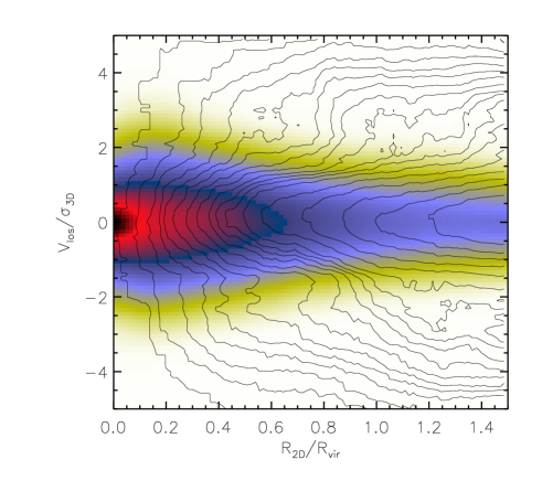
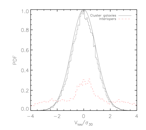
Figure 18.— Left panel: The color map represents the distribution of the line of sight velocity of cluster galaxies (within $3\mbox{$R_{\rm{vir}}$}$) normalized to the intrinsic 3D velocity dispersion of clusters as a function of the projected distance from the cluster center in units of $R_{\rm{vir}}$ for the sample described in the text. The contour lines represent the same distribution for the interloper galaxies. Right panel: The distribution of velocities in units of the intrinsic 3D velocity dispersion for the cluster galaxy population (solid black histogram) and for the interloper population (dashed red histogram). The normalisation is arbitrary, while the relative ratio of the two histograms reflects the sample described in the text. The solid black Gaussian is the expected distribution with width given by the Eq. 6 and $N_{gal}=25$.

As mentioned above, for each cluster along all the projections we end up with different samples of red-sequence galaxies that the $3\sigma$ clipping procedure recognises as ”spectroscopic members”. Therefore, for each different initially selected number of red-sequence galaxies, we measure the robust estimation of the velocity dispersion. We then apply Eq. 2 to estimate the dynamical mass. Left panel of Fig. 19 shows the corresponding relation between the resulting dynamical mass and the true virial mass for all the sample stacked together. The dashed black-purple line is the one to one relation, whereas the green lines show the 16, 50 and 84 percentiles. Note that the sample shown here is volume limited, and so the distribution in mass is different than the typical observational samples. Furthermore, the same clusters appear several times with dynamical masses computed from different number of galaxies on each projection, and within different projected radii at all the redshifts. When red-sequence galaxies are selected within a projected radius from a light-cone regardless of their true 3D distance from the centre of the cluster, the relation between the virial mass and the inferred dynamical mass is much broader. In particular, by looking at the median of the distribution, it is possible to notice that a systematical overestimation of the dynamical mass is present at all cluster masses, as expected from the interloper contribution previously discussed. Furthermore, especially at the low mass end of the cluster galaxy distribution, the presence of a significant population of catastrophic outliers is making the relation among virial mass and dynamical mass very asymmetric and causing a severe boosting of the dynamical mass.

These outliers are likely related to cases where the simple $3\sigma$ clipping procedure is not sophisticated enough to effectively separate the foreground and background interloper galaxies from the proper cluster galaxies. To verify this hypothesis we show in the right panel of Fig. 19 the same computation as for the left panel, but restricting our sample to only the cases in which the presence of interlopers is smaller than $5\%$. We note how this sub-sample qualitatively looks very similar to left panel of Fig. 9 which by construction contains only cluster galaxies. Furthermore, once the contribution from interlopers is removed, the bias of dynamical mass over the true mass disappears. However, remember that Fig. 19 shows that without interlopers dynamical masses are on average underestimated compared to the true virial mass, as expected from the effect of dynamical friction described in Sect. 4.1. Moreover, as expected from the lower panels of Fig. 15, the adopted interlopers rejection method is more effective for more massive clusters. Clearly the interloper effect on the dynamical mass is more severe at the low mass end of the cluster population.

Because the color selection of cluster members is a crucial point in this analysis, the results presented here obviously depend on the adopted galaxy formation model at some level. On the one hand it is true that the model is not perfectly reproducing the observed properties of the cluster galaxy population. On the other hand we also do not take into account any observational uncertainty which will instead affect the real data, for example broadening the observed red-sequence at fainter magnitudes.

To estimate the sensitivity of the color selection to uncertainties in the galaxy modeling on the above described results, we select red-sequence galaxies with a different criteria than the one described in Sect. 4. Instead of selecting the area in color-magnitude space which encompasses 68% of the cluster galaxies, we select all galaxies within a fixed $\pm 0.15$ $mag$ along the fitted red-sequence relation, similarly to the adopted criteria in the companion paper Bazin et al. (2012). This is on average a factor of $\sim 2$ in magnitude larger than the former threshold (depending on the redshift ranging from $\sim 0.5-3$, as highlighted in Tab. 2). Then, we reject interlopers and compute velocity dispersions and subsequent dynamical masses as described in the above sections. We find that the fraction of interlopers which the $3\sigma$ clipping procedure is not able to reject is on average in agreement within $\sim 3\%$ with the previous color selection. In particular for clusters with $M_{\rm{vir}}$ larger than $4\times 10^{14}\mbox{$M_{\rm{vir}}$ }$ the agreement is better than 1%.

We show in the left panel of Fig. 19 the resulting 16, 50 and 84 percentiles overplotted as red continuous lines. We note that a larger effect from the interlopers is present in comparison with the previous analyses, as expected from the broader color selection adopted. In particular, larger differences appear at the low mass end of the cluster galaxy population, where a significant increase of catastrophic outliers in the overestimation of the dynamical mass is visible. On the other hand, the average population is not affected by much. As a net result, a changing in the color selection of a factor $\sim 2$ implies a change in the estimated velocity dispersion by less than $\sim 3\%$. In particular, this difference reduces to less than $\sim 1\%$ for clusters with $M_{\rm{vir}}$ larger than $5\times 10^{14}\,{\rm M}_{\odot}$.

4.4. Unbiased Dispersion Mass Estimator

Similarly to Sect. 4.1, we try to parametrise as a function of the variables in Table 3 (aperture, number of spectra, redshift and cluster mass), the way that interlopers affect the inferred dynamical mass. However, we could not find a satisfactory analytical solution to easily model the measured velocity dispersion of clusters as a function of the above described variables, due to the non-linear interplay of the explored parameter space highlighted in Fig. 16. Therefore, we numerically compute the mean and the associated standard deviation of the ratio between the observed and the 1D intrinsic velocity dispersion in different bins of the parameter space as highlighted in Table 3. In this way, given the cluster mass, redshift and the number of red-sequence galaxy spectra within a given projected radius used to compute the velocity dispersion, we can correct for the average bias affecting the estimation of the dynamical mass. We show in Fig. 20 the same relation described in the left panel of Fig. 19 when such corrections are included. We remark that the bias is effectively removed at all the mass scales analysed here. Furthermore, by comparing the 84 percentile and median lines at the low mass end of the left panel of Fig. 19 with the ones in Fig. 20, we note that while the former are separated by about an order of magnitude in dynamical mass, for the later this difference is reduced to about $0.8$ dex.

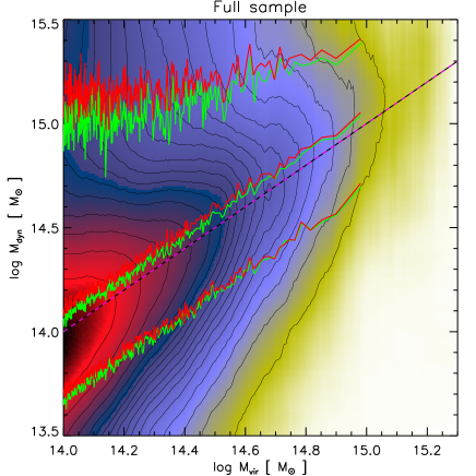
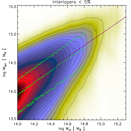
Figure 19.— Left panel: The distribution of the dynamical mass estimated through Eq. 2 as a function of the true $M_{\rm{vir}}$ for the whole sample described in Sect. 4 used in this work (green lines). Red lines represent the same distribution obtained from a different color selection of red-sequence galaxies as explained in Sect. 4.3.Right panel: Same as for the left panel, but only for the cases where the fraction of interlopers is smaller than $5\%$. Dashed purple-black line is showing the one-to-one relation, while solid green and red lines are the 16, 50 and 84 percentile.

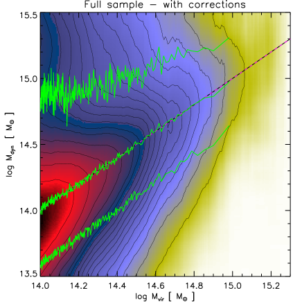
Figure 20.— Same as for the left panel of Fig. 19, but velocity dispersions were numerically corrected as described in the text. Dashed purple-black line is showing the oat-to-one relation, while solid green lines are the 16, 50 and 84 percentile. Note that with these corrections the dynamical mass is an unbiased estimator of the true mass.

5. Discussion and Conclusions

We have examined the use of velocity dispersions for unbiased mass estimation in galaxy clusters using the publicly available galaxy catalogue produced with the semi-analytic model by De Lucia & Blaizot (2007) coupled with the N-body cosmological Millennium Simulation (Springel et al. 2005). In particular, we selected all galaxies in the SAM with stellar mass larger than $10^{8}\,{\rm M}_{\odot}$ and analysed a sample consisting of more than $\sim 20000$ galaxy clusters with $\mbox{$M_{\rm{vir}}$ }\geq 10^{14}\,{\rm M}_{\odot}$ up to $z\sim 1.2$ (Tab: 1).

First we explore the properties of the full galaxy sample and then we increase the level of complications to mimic the spectroscopic selection that is typically undertaken in real world studies of clusters. Then we work through a series of controlled studies in an attempt to disentangle the different effects leading to biases and enhanced scatter in velocity dispersion mass estimates. Ultimately our goal is to inform the dispersion based mass calibration of the SPT cluster sample (Bazin et al. 2012), but we explore a broad range in selection in hopes that our results will be of general use to the community.

Our primary conclusions for the full subhalo population are:

• We measure the galaxy (i.e. subhalo) velocity dispersion mass relation and show that it has low scatter ($\sim 0.14$ in $ln(M)$) and that subhalo dispersions are $\lesssim$3% lower than DM dispersion in Evrard et al. (2008). This difference corresponds to a $\lesssim 10$% bias in mass for our halos if the DM dispersion– mass relation is used, and is consistent with previous determination of subhalo velocity bias.

• We explore line of sight velocity dispersions of the full galaxy populations within the cluster ensemble and confirm that the triaxiality of the velocity dispersion ellipsoid is the dominant contributor to the characteristic $\sim$35% scatter in dispersion based mass estimates. We show that this scatter increases with redshift as $\sigma(z)\simeq 0.3+0.075z$.

• We measure the principal axes and axial ratios of the spatial galaxy distribution ellipsoid, showing that there is a slight ($\sim 5$%) preference for prolate distributions; this property has no clear variation with mass or redshift. We examine the line of sight velocity dispersions along the principle axes, showing that the slight preference toward prolate geometries translates into a slight ($\sim 1$%) bias in the dispersion mass estimates extracted from line of sight measures.

Our primary conclusions for the spectroscopic subsamples of subhalos are:

• We characterize the bias (Eqn. 6) and the scatter (Eqn. 7) in the line of sight velocity dispersion introduced by selecting a subset $N_{gal}$ of the most luminous red sequence galaxies within a cluster. The bias is significant for samples with $N_{gal}<30$ and is likely due to dynamical friction of these most massive subhalos. The scatter cannot be fully explained through a combination of intrinsic scatter in the relation between mass and the 3D dispersion of all galaxies (i.e. departures from equilibrium), scatter of the line of sight dispersion around the 3D dispersion (halo triaxility) and Poisson noise associated with the number of subhalos $N_{gal}$. A further component of scatter due to the presence of a dynamically cold population of luminous red-sequence galaxies is needed to explain the full measured scatter.

• We explore the impact of interlopers by creating spectroscopic samples using (1) red sequence color selection, (2) a maximum projected separation from the cluster center, and (3) $N$-sigma outlier rejection in line of sight velocity. In these samples the interloper fraction (contamination) can be significant, growing from $\sim 10\%$ at the projected virial radius to $\sim$35% at twice the project virial radius. The contamination fraction has a much weaker dependency on the sample size $N_{gal}$. We explore the dependence on mass and cluster redshift, showing that within a fixed aperture, contamination is a factor of $\sim 2$ worse at redshift $z\sim 1$ than at $z=0$. Furthermore, we show that the fraction of interlopers is a steeper function of aperture for low mass clusters, but that at fixed redshift contamination does not change significantly with mass. We show that contamination is significant even if a more sophisticated caustic approach is used to reject interlopers, demonstrating that even clusters with large numbers of spectroscopic redshifts for red sequence selected galaxies suffer contamination from non-cluster galaxies. We further study how interlopers are affecting the estimated velocity bias. We find that the velocity bias has a minimum if computed within $R_{\perp}\sim\mbox{$R_{\rm{vir}}$}$. This is due to the balancing effect of larger intrinsic velocity bias at smaller radii and larger contamination at larger radii. Furthermore, we show that if velocity dispersions are computed within projected aperture $R_{\perp}$ larger than $\sim\mbox{$R_{\rm{vir}}$}$, the velocity bias is a steeper function of $R_{\perp}$ for higher redshifts and lower cluster mass, as expected from the contamination fraction.

• We study how changing the color selection affects the fraction of interlopers and the subsequent effect on the estimated velocity dispersion and dynamical masses. We find that doubling the width of the color selection window centered on the red sequence has only a modest impact on the interloper fraction. The primary effect of changing the color selection is on the filtering of catastrophic outliers. This results in changes to the estimated velocity dispersion virial mass relation at the level of 1% in mass. We also show that uncertainties in the color selection are more important for low mass clusters than for the high mass end of the cluster population, which is because the dispersions of low mass clusters are more sensitive to catastrophic outliers. The rather weak dependence of the dispersion based mass estimates on the details of the color selection suggests also that uncertainties in the star formation histories (and therefore colors) of galaxy populations in and around clusters are not an insurmountable challenge for developing unbiased cluster mass estimates from velocity dispersions.

• We present a model to produce unbiased line of sight dispersion based mass estimates, correcting for interlopers and velocity bias. We also present the probability distribution function for the scatter of the mass estimates around the virial mass. These two data products can be used together with a selection model describing real world cluster dispersion measurements to enable accurate cluster mass calibration.

In a companion paper, Bazin et al. (2012) apply this model in the dispersion mass calibration of the SPT Sunyaev-Zel’odovich effect selected cluster sample. We identify the following key remaining challenges in using dispersions for precise and accurate mass calibration of cluster cosmology samples. Surprisingly, the larger systematic uncertainty has to be ascribed to our relative poor knowledge of the velocity bias between galaxies or subhalos and DM. A conservative estimate of this systematic is at the level of $<5\%$ and arises from the comparison of different simulations and different algorithms for subhalo identification (e.g. Evrard et al. 2008). The systematic uncertainty in the color selection of galaxies and its subsequent mapping between line of sight velocity dispersion and mass is at relatively smaller level. Indeed we can estimate it at a $<1\%$ level for samples selected as the ones described in Bazin et al. (2012), despite the fact that galaxy formation models involve a range of complex physical processes. In other words, systematics in predicting galaxy properties (e.g. luminosity, colors, etc.) due to subgrid physics associated with magnetic fields, AGN and supernova feedback, radiative cooling and the details of star formation, do not appear to significantly change the spectroscopic sample selection. On the other hand, simulations including different physical treatments of gravity are affecting the dynamics of the spectroscopic selected sample at a higher level than we expected. Given that the current dominant contributor to the systematics floor is an issue associated with the treatment of gravitational physics, there are reasons to be optimist that future simulations will be able to reduce the current systematics floor.

We acknowledge Jonathan Ruel for very useful discussions and support from the Deutsche Forschungsgemeinschaft funded Excellence Cluster Universe and the trans-regio program TR33: Dark Universe.

References

- Abell (1958) Abell, G. O. 1958, ApJS, 3, 211
- Adami et al. (1998) Adami, C., Biviano, A., & Mazure, A. 1998, A&A, 331, 439
- Andersson et al. (2011) Andersson, K., Benson, B. A., Ade, P. A. R., et al. 2011, ApJ, 738, 48
- Barnes & Hut (1986) Barnes, J., & Hut, P. 1986, Nature, 324, 446
- Bazin et al. (2012) Bazin et al. 2012, In Preparation
- Beers et al. (1990) Beers, T. C., Flynn, K., & Gebhardt, K. 1990, AJ, 100, 32
- Benson (2010) Benson, A. J. 2010, Phys. Rep., 495, 33
- Biviano et al. (1992) Biviano, A., Girardi, M., Giuricin, G., Mardirossian, F., & Mezzetti, M. 1992, ApJ, 396, 35
- Biviano et al. (2006) Biviano, A., Murante, G., Borgani, S., et al. 2006, A&A, 456, 23
- Böhringer et al. (2000) Böhringer, H., Voges, W., Huchra, J. P., et al. 2000, ApJS, 129, 435
- Cappi et al. (2003) Cappi, A., Benoist, C., da Costa, L. N., & Maurogordato, S. 2003, A&A, 408, 905
- Davis et al. (1985) Davis, M., Efstathiou, G., Frenk, C. S., & White, S. D. M. 1985, ApJ, 292, 371
- De Lucia & Blaizot (2007) De Lucia, G., & Blaizot, J. 2007, MNRAS, 375, 2
- De Lucia et al. (2004a) De Lucia, G., Kauffmann, G., Springel, V., et al. 2004a, MNRAS, 348, 333
- De Lucia et al. (2004b) De Lucia, G., Kauffmann, G., & White, S. D. M. 2004b, MNRAS, 349, 1101
- Diaferio & Geller (1997) Diaferio, A., & Geller, M. J. 1997, ApJ, 481, 633
- Dressler & Shectman (1988) Dressler, A., & Shectman, S. A. 1988, AJ, 95, 985
- Evrard et al. (2008) Evrard, A. E., Bialek, J., Busha, M., et al. 2008, ApJ, 672, 122
- Faltenbacher & Diemand (2006) Faltenbacher, A., & Diemand, J. 2006, MNRAS, 369, 1698
- Fassbender et al. (2011) Fassbender, R., Böhringer, H., Nastasi, A., et al. 2011, New Journal of Physics, 13, 125014
- Gao et al. (2004) Gao, L., De Lucia, G., White, S. D. M., & Jenkins, A. 2004, MNRAS, 352, L1
- Geller & Beers (1982) Geller, M. J., & Beers, T. C. 1982, PASP, 94, 421
- Gladders & Yee (2005) Gladders, M. D., & Yee, H. K. C. 2005, ApJS, 157, 1
- Goto (2005) Goto, T. 2005, MNRAS, 359, 1415
- Hao et al. (2010) Hao, J., McKay, T. A., Koester, B. P., et al. 2010, ApJS, 191, 254
- Jing & Suto (2002) Jing, Y. P., & Suto, Y. 2002, ApJ, 574, 538
- Kasun & Evrard (2005) Kasun, S. F., & Evrard, A. E. 2005, ApJ, 629, 781
- Kauffmann et al. (1999) Kauffmann, G., Colberg, J. M., Diaferio, A., & White, S. D. M. 1999, MNRAS, 303, 188
- Koester et al. (2007) Koester, B. P., McKay, T. A., Annis, J., et al. 2007, ApJ, 660, 221
- Łokas et al. (2006) Łokas, E. L., Wojtak, R., Gottlöber, S., Mamon, G. A., & Prada, F. 2006, MNRAS, 367, 1463
- Mamon et al. (2010) Mamon, G. A., Biviano, A., & Murante, G. 2010, ArXiv e-prints
- Marriage et al. (2011) Marriage, T. A., Acquaviva, V., Ade, P. A. R., et al. 2011, ApJ, 737, 61
- Mohr et al. (1995) Mohr, J. J., Evrard, A. E., Fabricant, D. G., & Geller, M. J. 1995, ApJ, 447, 8+
- Pacaud et al. (2007) Pacaud, F., Pierre, M., Adami, C., et al. 2007, MNRAS, 382, 1289
- Perea et al. (1990) Perea, J., del Olmo, A., & Moles, M. 1990, A&A, 237, 319
- Planck Collaboration et al. (2011) Planck Collaboration, Ade, P. A. R., Aghanim, N., et al. 2011, ArXiv e-prints
- Reichardt et al. (2012) Reichardt et al. 2012, In Preparation
- Reiprich & Böhringer (2002) Reiprich, T. H., & Böhringer, H. 2002, ApJ, 567, 716
- Serra et al. (2011) Serra, A. L., Diaferio, A., Murante, G., & Borgani, S. 2011, MNRAS, 412, 800
- Song et al. (2011) Song, J., Mohr, J. J., Barkhouse, W. A., Warren, M. S., & Rude, C. 2011, ArXiv e-prints
- Springel (2005) Springel, V. 2005, MNRAS, 364, 1105
- Springel et al. (2001a) Springel, V., White, S. D. M., Tormen, G., & Kauffmann, G. 2001a, MNRAS, 328, 726
- Springel et al. (2001b) Springel, V., Yoshida, N., & White, S. D. M. 2001b, Nature, 6, 79
- Springel et al. (2005) Springel, V., White, S. D. M., Jenkins, A., et al. 2005, Nature, 435, 629
- Stanford et al. (2005) Stanford, S. A., Eisenhardt, P. R., Brodwin, M., et al. 2005, ApJ, 634, L129
- Staniszewski et al. (2009) Staniszewski, Z., Ade, P. A. R., Aird, K. A., et al. 2009, ApJ, 701, 32
- Sunyaev & Zel’dovich (1972) Sunyaev, R. A., & Zel’dovich, Y. B. 1972, Comments on Astrophysics and Space Physics, 4, 173
- Szabo et al. (2011) Szabo, T., Pierpaoli, E., Dong, F., Pipino, A., & Gunn, J. 2011, ApJ, 736, 21
- Thomas & Couchman (1992) Thomas, P. A., & Couchman, H. M. P. 1992, MNRAS, 257, 11
- Tormen (1997) Tormen, G. 1997, MNRAS, 290, 411
- Šuhada et al. (2012) Šuhada, R., Song, J., Böhringer, H., et al. 2012, A&A, 537, A39
- Vanderlinde et al. (2010) Vanderlinde, K., Crawford, T. M., de Haan, T., et al. 2010, ApJ, 722, 1180
- Vikhlinin et al. (2009) Vikhlinin, A., Burenin, R. A., Ebeling, H., et al. 2009, ApJ, 692, 1033
- Warren et al. (1992) Warren, M. S., Quinn, P. J., Salmon, J. K., & Zurek, W. H. 1992, ApJ, 399, 405
- White et al. (2010) White, M., Cohn, J. D., & Smit, R. 2010, MNRAS, 408, 1818
- Williamson et al. (2011) Williamson, R., Benson, B. A., High, F. W., et al. 2011, ApJ, 738, 139
- Wojtak et al. (2009) Wojtak, R., Łokas, E. L., Mamon, G. A., & Gottlöber, S. 2009, MNRAS, 399, 812
- Wojtak et al. (2007) Wojtak, R., Łokas, E. L., Mamon, G. A., et al. 2007, A&A, 466, 437
- Zhang et al. (2011) Zhang, Y.-Y., Andernach, H., Caretta, C. A., et al. 2011, A&A, 526, A105
- Zwicky et al. (1968) Zwicky, F., Herzog, E., & Wild, P. 1968, Catalogue of galaxies and of clusters of galaxies (California Institute of Technology, Pasadena)