On modeling hydraulic fracture in proper variables:
stiffness, accuracy, sensitivity

Abstract

The problem of hydraulic fracture propagation is considered by using its recently suggested modified formulation in terms of the particle velocity, the opening in the proper degree, appropriate spatial coordinates and $\varepsilon$-regularization. We show that the formulation may serve for significant increasing the efficiency of numerical tracing the fracture propagation. Its advantages are illustrated by re-visiting the Nordgren problem. It is shown that the modified formulation facilitates (i) possibility to have various stiffness of differential equations resulting after spatial discretization, (ii) obtaining highly accurate and stable numerical results with moderate computational effort, and (iii) sensitivity analysis. The exposition is extensively illustrated by numerical examples.

1 Introduction

Hydraulic fracturing is a widely used method serving to increase the linear size of an area of fluid or gas flow (see, e.g. the reviews in papers [14], [7], [2]). In view of practical significance of the method, numerous papers have been published on the theory and numerical modeling of hydraulic fractures starting from the first publications [18], [4], [26], [11], [14], [25], [29] and [24]. The general formulation of the problem is well established (e.g. [2]). It includes (i) the fluid equations for flow of incompressible viscous fluid in the narrow channel; (ii) the solid mechanics (commonly static linear elasticity) equations defining the dependence of the channel’s height on the pressure acting on the walls of the channel; (iii) equations of fracture mechanics defining the possibility of the fracture propagation and the trajectory of the fracture contour. Additional equations for proppant movement are added when accounting for the proppant injected at some stage of fracturing.

The formulated mathematical problem is difficult from the computational point of view because of three major complicating factors: strong nonlinearity even in the simplest case of Newtonian fluid, caused by the fact that the channel’s height (fracture opening) raised to some power enters the Poiseuille equation as a multiplier by the unknown flux; moving boundaries of the fluid front and fracture contour; and, in general, the need to check the fracture conditions for finding the value and direction the fracture increment at time steps at each point of the front. Consequently, many investigations have been performed tending to reveal those general properties of the solution, which may serve for the problem simplification. They have provided knowledge on the asymptotics of the solution, possibility to neglect the lag between the fluid front and the fracture contour and on the typical regimes (e.g. [29], [5], [9], [1], [27], [6], [3], [8], [23], [17], [15], [10]). The knowledge was incorporated in the computational codes for practical applications (e.g. [16], [2]). Still, the mentioned difficulties are not overcome, and as emphasized in the review [2], there is the need ”to dramatically speed up” simulators.

The recent studies tended to address this challenge [19] – [22] have disclosed important features of the hydraulic fracture problem, which may be employed for enhancing the numerical simulation. They have led to the modified formulation of the problem using:

1. the particle velocity, as a variable with continuous spatial derivative near the fluid front, instead of the pressure;

2. the opening taken in a degree, defined by its asymptotic behavior at the fluid front, instead of the opening itself;

3. the speed equation (SE) at each point of the front to trace the fracture propagation by the well-developed methods (see, e.g. [28]), instead of the commonly employed single equation of the global mass balance; the speed equation also presents the basis for proper regularization;

4. $\varepsilon$-regularization, that is imposing the boundary condition and the speed equation at a small distance from the front rather than on the front itself, to exclude deterioration of the solution near the front caused by the disclosed fact ([19], [20]) that the boundary value problem is ill-posed when neglecting the lag;

5. the spatial coordinates moving with the front and evaluation of the temporal derivative under fixed values of these coordinates;

6. reformulation of the common system of equations and boundary conditions in terms of the suggested variables complimented with $\varepsilon$-regularization.

The computational advantages of the modified formulation have been demonstrated [19], [20] by revisiting the classical Nordgren [25] problem. For it, common (without $\varepsilon$-regularization) time stepping procedures could not provide reliable third digit and they led to strong deterioration of the solution near the fluid front for fine meshes. In contrast, applying $\varepsilon$-regularization easily provided the solution with relative error less than $10^{-4}$ in a time stepping procedure; the solution was extremely stable and it never deteriorated near the front. Using of the suggested variables made it also possible [22] to obtain analytical solutions of the Nordgren [25] and Spence and Sharp [29] problems.

In this paper, we make a further step in employing the modified formulation for (i) studying the stiffness of the system of differential equations arising after spatial discretization, (ii) increasing the efficiency of numerical tracing of the fracture propagation, and (iii) studying the sensitivity. To simplify the exposition and to compare the numerical results with benchmarks, we address the Nordgren problem.

The structure of the paper is as follows. In Section 2, we briefly review various formulations of the problem. They include the common formulation (Subsection 2.1), the mentioned modified formulation (Subsection 2.2), its specification for the Nordgren problem (Subsection 2.3) and the self-similar formulation for 1D problems. The latter serves us to write down the benchmark analytical solution of the Nordgren problem in the case of zero leak-off [22] and to obtain a benchmark solution for non-zero leak-off (Subsection 2.4). Further analysis employs the modified formulation and the benchmark solutions.

Section 3 presents alternative approaches to spatial discretization of the lubrication partial differential equation (PDE) and the speed equation. It is shown that they result in various systems of ordinary differential equations (ODE) with quite different stiffness. It appears that in schemes avoiding approximation of the second spatial derivative by assuming the particle velocity fixed at an iteration step, the stiffness, in general, is not high being of order $O(N)$, where $N$ is the number of nodal points. In the case of constant particle velocity, the stiffness becomes of order $1/\varepsilon$ independently on $N$ ($\varepsilon$ is the regularization parameter). This indicates favorable features of iterative schemes with the velocity fixed at the stage of integration in time. In contrast, in schemes employing approximation of the second spatial derivative, the stiffness depends on the number $N$ more strongly: it is of order $N^{2}$ for the Nordgren problem and of order $N^{3}$ in the general case when the net pressure is connected with the opening by exact equations of the elasticity theory.

Section 4 presents two alternative approaches based on the approximation of the second spatial derivative. The first of them employs the possibility to add the SE to the system of ODE, resulting from the spatial discretization of the modified lubrication equation. In this way, we obtain a new well-posed formulation for the joined system of ODE with initial (Cauchy) conditions on the fluid front. The formulation opens the possibility to employ methods, like those of Runge-Kutta, for solving the ODE. It serves us to use a standard MATLAB solver in further evaluations of the accuracy and sensitivity. The second approach employs classical Crank-Nicolson scheme to reduce the problem to tri-diagonal algebraic system. In this case, non-linear factors in front of the derivatives are iterated within a time step. The SE is used at iterations to find the new location of the fluid front. The rest of Section 4 contains numerical results for these approaches and their discussion. It appears that the numerical procedures resulting from each of them are highly accurate, stable and robust. For comparison, we also present results obtained by using the equation of the global mass balance instead of the SE. It appears that the accuracy becomes notably (an order, at least) less than that when using the SE.

In Section 5 we study sensitivity of the solution to changes of influx which is one of the major parameters of the problem. Conclusions are drawn in Section 6.

2 Problem formulation

2.1 Conventional formulation

As mentioned, a mathematical formulation of the problem includes three groups of equations. Firstly we present them in the conventional form.

fluid equations include the volume conservation law

$$\frac{\partial w}{\partial t}+\mbox{div}\,\mathbf{q}+q_{l}=0$$ (1)

and the relation of the Poiseuille type obtained by integration of Navier-Stokes equations for a flow of viscous fluid in a narrow channel

$$\mathbf{q}=-D(w,p)\,\mbox{grad}\,p.$$ (2)

Herein, $w(\mathbf{x},t)$ is the channel width (fracture opening), $\mathbf{q}(\mathbf{x},t)$ is the flux vector through the fracture height, $q_{l}(\mathbf{x},t)$ is the intensity of distributed sinks or sources (below this term will be assumed positive to account for leak-off), $p(\mathbf{x},t)$ is the pressure, $D$ is a function or operator, such that $D(0,p)\mbox{grad}\,p=\mathbf{0,}$ $\mathbf{x}$ denotes the vector of the position of a point on the surface of the flow, $t$ is the time. The flux, divergence and gradient are defined in the tangent plane to the surface of the flow.

Substitution of (2) into (1) yields the lubrication (Reynolds) equation

$$\frac{\partial w}{\partial t}-\mbox{div}\,\big{(}D(w,p)\,\mbox{grad}\,p\big{)}+q_{l}=0.\quad$$ (3)

In hydraulic fracture problems, the opening is not known in advance. Thus its initial spatial distribution should be defined at start time $t_{0}$:

$$w(\mathbf{x},t_{0})=w_{0}(\mathbf{x}),\quad$$ (4)

where $w_{0}(\mathbf{x})$ is a prescribed function.

The spatial operator in (3) is of the second order and elliptic. It requires only one boundary condition at the fluid contour $L_{e}$. For instance, when neglecting the lag between the fluid front and the fracture contour, it may be the condition of the prescribed normal component $q_{n}$ of the flux:

$$q_{n}(\mathbf{x},t)=q_{0}(\mathbf{x},t),\quad\mathbf{x}\in L_{e},$$ (5)

where $q_{0}(\mathbf{x},t)$ is a known function at $L_{e}$; specifically, at the points of the fluid injection it is defined by the injection regime; at the points of the fluid front, coinciding with the fracture contour, we have $w=0$ and equation (2) implies $q_{0}(\mathbf{x},t)=0$.

In conventional formulations (e.g. [29], [1], [27], [6], [8], [16], [2], [17], [15], [10]), to follow the fluid front propagation, authors use the equation of the global mass balance. Being a single equation, it do may serve for this purpose when considering 1-D problems with one point of the front to be traced. However in general, as emphasized in [19] – [22], it is preferable to employ the speed equation, which is formulated at each point of the fluid front. Even for 1-D problems, it provides advantages discussed in following sections. We shall not dwell on this issue here as the discussion below focuses on a 1-D problem.

Solid mechanics equations define a dependence of the opening on the net pressure caused by deformation of rock:

$${\cal A}w=p,\quad$$ (6)

with the condition of zero opening at each point $\mathbf{x}_{c}$ of the fracture contour:

$$w(\mathbf{x}_{c})=0.\quad$$ (7)

Commonly, the operator ${\cal A}$ in (6) is obtained by using the theory of linear static elasticity. As mentioned, when neglecting the lag, the condition of zero opening (7) replaces the condition of zero flux on the front. Henceforth, we shall consider this case and write $x_{c}=x_{\ast}$ with the star marking that a quantity refers to the fluid front.

Fracture mechanics equations define the critical state and the perspective direction of the fracture propagation. In the commonly considered case of the tensile mode of fracture, these are:

$$K_{I}(\mathbf{x}_{c})=K_{IC},\text{ \ \ \ \ }K_{II}(\mathbf{x}_{c})=0,\quad$$ (8)

where $K_{I}\$is the tensile stress intensity factor (SIF), $K_{IC}$ is its critical value, $K_{II}$ is the shear SIF.

The problem consists in solving the PDE (3) together with the elasticity equation (6) under the initial condition (4), boundary conditions (5), (7) and the fracture conditions (8). As mentioned, the global mass balance is usually employed instead of the speed equation to find a current position of the front.

2.2 Modified formulation of fluid equations and boundary conditions

The modified formulation [19] – [22] concerns mostly with the fluid equations and corresponding boundary conditions. It employs the primary quantity resulting from integration of the Navier-Stokes equations when a flow occurs in a narrow channel; this is the particle velocity. Its value $\mathbf{v}$ averaged across the channel height defines the flux $\mathbf{q}$ entering equations (1), (2), (5), because by definition

$$\mathbf{q}=w\mathbf{v}.$$ (9)

Thus we may use the fluid particle velocity

$$\mathbf{v=}\frac{\mathbf{q}}{w}$$ (10)

instead of the flux $\mathbf{q}$. In terms of the particle velocity, the conservation law (1) and the Poiseuille type equation (2) become, respectively:

$$\frac{\partial w}{\partial t}+\mbox{div}\,(w\mathbf{v)}+q_{l}=0,\quad$$ (11)

and

$$\mathbf{v}=-\frac{1}{w}D(w,p)\,\mbox{grad}\,p.$$ (12)

For the velocity component $v_{n}$ in a direction $\mathbf{n}$, the equation (12) yields

$$v_{n}=-\frac{1}{w}D(w,p)\frac{\partial p}{\partial n}.$$ (13)

In contrast with the flux, pressure and opening, the particle velocity is a smooth function near the fluid front. It follows from the fact that the particle velocity $\mathbf{v(x}_{\mathbf{\ast}}\mathbf{)}$ equals to the front speed $\mathbf{V}_{\ast}$ at each point $\mathbf{x}_{\ast}$ of the front. In terms of the components $v_{n\ast}$, $V_{\ast}$, normal to the front, we have:

$$v_{n\ast}(\mathbf{x}_{\ast})=\frac{dx_{n\ast}}{dt}=V_{\ast}(\mathbf{x}_{\ast}),$$ (14)

where $x_{n\ast}$ is the normal component of a point $\mathbf{x}_{\ast}$ on the front, $V_{\ast}=\left|\mathbf{V}_{\ast}\right|$. Hence, the particle velocity is finite at the front in common cases of the front propagation with a finite speed. Moreover, it is non-zero  except for flows with stagnation points.

The equation (14), where the normal component of the particle velocity is defined by (13), presents the speed equation for the problem of hydraulic fracture:

$$V_{\ast}(\mathbf{x}_{\ast})=-\frac{1}{w(\mathbf{x}_{\ast})}D(w,p)\frac{\partial p}{\partial n_{\ast}}.$$ (15)

Herein, $\mathbf{n}_{\ast}$ is the unit normal to the front in the direction of its propagation at a point $\mathbf{x}_{\ast}$. Being the starting concept of the theory of propagating surfaces [28], the speed equation is fundamental for proper tracing the hydraulic fracture propagation.

The speed equation (15) yields also important implications for numerical simulation of hydraulic fractures by finite differences (FD). Indeed, when at a time step we have known both $\mathbf{x}_{\ast}$ and $V_{\ast}(\mathbf{x}_{\ast})$, the equation (15) becomes a boundary condition additional to the boundary condition (7) on the front. Thus, as noted in [19], a boundary value problem may appear overdetermined and ill-posed in the Hadamard sense [12]. To avoid difficulties, it is reasonable to use $\varepsilon$-regularization, suggested and successfully used in [19], [20].

The $\varepsilon$-regularization is performed as follows. An exact boundary condition on the fluid front is changed to an approximate equality at a small distance $r_{\varepsilon}$ behind the front. This approximate equality is obtained by combining the boundary condition at the fluid front, particular for a considered problem, with the speed equation, which is quite general. In practical calculations, the distance (absolute $r_{\varepsilon}$ or relative $\varepsilon$) is taken small enough to use the equality sign in the derived approximate condition. This gives us the $\varepsilon$-regularized boundary condition near the front. The speed equation is also assumed to be met at the distance $r_{\varepsilon}$ with an accepted accuracy. This gives us the $\varepsilon$-regularized speed equation. The $\varepsilon$-regularized boundary condition allows one to avoid the mentioned unfavorable computational effects; the $\varepsilon$-regularized speed equation serves to find the front propagation.

In this way, the boundary conditions (7) and (15) are combined to obtain the $\varepsilon$-regularized boundary condition [20], [21]:

$$\int_{p_{0}}^{p_{\varepsilon}}\frac{1}{w}D(w,p)dp=V_{\ast}r_{\varepsilon},$$ (16)

where $p_{\varepsilon}=p(r_{\varepsilon})$ is the pressure at the distance $r_{\varepsilon}$ from the front. The $\varepsilon$-regularized form of the speed equation (15) is:

$$V_{\ast}(t)=\frac{dx_{n\ast}}{dt}=-\frac{1}{w}D(w,p)\frac{\partial p}{\partial n}_{r_{\varepsilon}}.$$ (17)

The equations (16) and (17) actually employ the system moving with the front. Thus it is reasonable to re-write the lubrication equation (11) in this system. In it, the $r$-axis is directed opposite to the front velocity, while the other axis is tangent to the front. The connection between the temporal derivatives evaluated under constant $x$ and $r$ is given by the rule:

$\frac{\partial}{\partial t}\big{|}_{\mathbf{x}=const}=\frac{\partial}{\partial t}\big{|}_{r=const}+V_{\ast}\frac{\partial}{\partial r}.$

Then equation (11) reads [20]:

$$\frac{\partial\ln w}{\partial t}=\frac{\partial v_{n}}{\partial r}+(v_{n}-V_{\ast})\frac{\partial\ln w}{\partial r}-\frac{1}{w}q_{l},$$ (18)

where using ln$w$ serves to account for an arbitrary power asymptotic behavior of the opening

$$w(r,t)=C(t)r^{\alpha}+O(r^{\delta}),\quad r\to 0,\quad\text{\ }\alpha\geq 0,\text{ }\delta>\alpha$$ (19)

near the front. The value of the exponent $\alpha$ is known in a number of important particular cases (see, e.g. [29], [5], [1], [17]), and $\delta=1+\alpha$ when the leak-off is neglected.

For the asymptotics (19), it is reasonable, in addition to the particle velocity, to use the variable $y(r,t)=[w(\mathbf{x}_{\ast}-r\mathbf{n},t)]^{1/\alpha}$, which is linear in $r$ near the front. Finally the lubrication equation (18) near the fluid front becomes

$$\frac{\partial y}{\partial t}=\frac{y}{\alpha}\frac{\partial v_{n}}{\partial r}+(v_{n}-V_{\ast})\frac{\partial y}{\partial r}-\frac{y^{1-\alpha}}{\alpha}\,q_{l}.$$ (20)

In 1-D cases, the equation (20) is applicable to the entire fluid. In these cases, there is the only spatial coordinate $x$ and it is reasonable to normalize $x$ or, what is actually equivalent, $r$ by the distance $x_{\ast}(t)$ from the inlet to the front. When using $\varsigma=x/x_{\ast}$, the partial derivative evaluated under constant $r$ is expressed via that under constant $\varsigma$ as:

$$\frac{\partial}{\partial t}\big{|}_{r=const}=\frac{\partial}{\partial t}\big{|}_{\varsigma=const}+(1-\varsigma)\frac{V_{\ast}}{x_{\ast}}\frac{\partial}{\partial\varsigma}.$$

Then in terms of $\varsigma=x/x_{\ast}=1-r/x_{\ast}$, the lubrication equation (20) in 1-D cases reads:

$$\frac{\partial\tilde{y}}{\partial t}=\frac{1}{x_{\ast}}\left[(\varsigma\tilde{V}_{\ast}-\tilde{v})\frac{\partial\tilde{y}}{\partial\varsigma}-\frac{\tilde{y}}{\alpha}\frac{\partial\tilde{v}}{\partial\varsigma}\right]-\frac{\tilde{y}^{1-\alpha}}{\alpha}\,\tilde{q}_{l},$$

where we have omitted the subscript $n$ in the notation of the particle velocity; tilda over a symbol marks that the corresponding function is considered to be a function of $\varsigma$: $\tilde{y}(\varsigma,t)=y(x_{\ast}(1-\varsigma),t)$, $\tilde{v}(\varsigma,t)=v(x_{\ast}(1-\varsigma),t)$, $\tilde{q}_{l}(\varsigma,t)=q_{l}(x_{\ast}(1-\varsigma),t)$. From now on, to simplify notation, we shall omit the tilda over functions depending on $\varsigma$. Thus, the previous equation is written as:

$$\frac{\partial y}{\partial t}=\frac{1}{x_{\ast}}\left[(\varsigma V_{\ast}-v)\frac{\partial y}{\partial\varsigma}-\frac{y}{\alpha}\frac{\partial v}{\partial\varsigma}\right]-\frac{y^{1-\alpha}}{\alpha}\,q_{l},$$ (21)

Note that when $q_{l}$ near the front decreases faster than $w=y^{\alpha}$, we may divide (21) by $y$, obtaining the equation

$$\frac{1}{y}\frac{\partial y}{\partial t}=\frac{\varsigma V_{\ast}-v}{x_{\ast}y}\frac{\partial y}{\partial\varsigma}-\frac{1}{\alpha x_{\ast}}\frac{\partial v}{\partial\varsigma}-\frac{1}{\alpha y^{\alpha}}\,q_{l}.$$ (22)

In (22), under the assumed asymptotics of $q_{l}$, the term $(\partial y/\partial t)/y$, the factor ($\varsigma V_{\ast}-v)/(x_{\ast}y)$ and the derivative $\partial v/\partial\varsigma$ are finite at the fluid front.

2.3 Nordgren problem in modified formulation

The 1-D problem (Fig. 1) studied by Nordgren [25] is similar to that considered by Perkins and Kern [26], improving the model of these authors by rigorous mathematical formulation, which includes finding the fracture length $x_{\ast}$ as a part of the solution. Below we use the rigorous formulation by Nordgren and attribute it to this author.

The fluid equations of the problem are (1) - (3) with the operator $D$ being the multiplier

$$D(w,p)=k_{l}w^{3},$$ (23)

corresponding to the flow of Newtonian fluid in a narrow channel with an elliptic cross-section; for it $k_{l}=1/(\pi^{2}\mu)$, where $\mu$ is the dynamic viscosity.

The operator ${\cal A}$ in the solid mechanics equation (6) is also taken in the simplest form as the multiplier $k_{e}=(2/\pi h)E/(1-\nu^{2})$ in the linear dependence between the pressure and opening

$$p=k_{e}w.$$ (24)

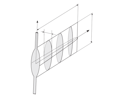
Figure 1: Scheme of the Nordgren problem.

Herein, $h$ is the vertical length of a narrow elliptic channel (Fig. 1), $E$ is the Young modulus, $\nu$ is the Poisson’s ratio of rock. For the dependence (24), there is no need in a fracture criterion because it does not involve the fracture front.

The initial condition (4) in the 1-D case reads

$$w(x,t_{0})=w_{0}(x),\quad$$ (25)

with $w_{0}(x)=0$ ahead of the fluid front $x_{\ast}(t_{0})$.

In view of (2), (23) and (24), the boundary condition (5) of the prescribed influx $q_{0}$ at the inlet $x=0$ becomes:

$$-\frac{k_{l}k_{e}}{3}w(0,t)\frac{\partial w^{3}}{\partial x}\big{|}_{x=0}=q_{0}(t).$$ (26)

The boundary condition of zero opening involves the only point $x_{\ast}=x_{*}(t)$ of the fluid front:

$$w(x_{*})=0.\quad$$ (27)

The equation for the particle velocity (12) and the speed equation (15) become, respectively,

$$v=-\frac{k_{l}k_{e}}{3}\frac{\partial w^{3}}{\partial x}$$ (28)

and

$$V_{\ast}=\frac{dx_{\ast}}{dt}=-\frac{k_{l}k_{e}}{3}\frac{\partial w^{3}}{\partial x}\big{|}_{x=x_{*}(t)}.$$ (29)

The exponent $\alpha$ in (19) equals 1/3 (see, e.g. [17]) when the leak-off is neglected or even when it is described by the Carter’s dependence and, consequently, singular at the crack tip. Then $y=w^{3}$, and in terms of the normalized independent variable $\varsigma$, the modified equation (21) for the 1-D problem (21) reads:

$$\frac{\partial y}{\partial t}=\frac{1}{x_{\ast}}\left[(\varsigma V_{\ast}-v)\frac{\partial y}{\partial\varsigma}-3y\frac{\partial v}{\partial\varsigma}\right]-3y^{2/3}q_{l},$$ (30)

where the particle velocity $v$ is connected with $y$ by equation following from (28):

$$v=-\frac{k_{l}k_{e}}{3x_{\ast}}\frac{\partial y}{\partial\varsigma}.$$ (31)

In the new variables, the asymptotic equation (19) with $\alpha=1/3$ is written as $y=C^{3}(t)x_{\ast}(1-\varsigma)+O((1-\varsigma)^{1+\kappa})$ for $\varsigma\rightarrow 1$, where $\kappa>0$ for any leak-off tending to zero at the crack tip. Then (29) and (31) imply that near the front $v=V_{\ast}=\frac{k_{l}k_{e}}{3}C^{3}(t).$ Hence, the coefficient $C^{3}(t)$ is a multiple of the front speed: $C^{3}(t)=\frac{3}{k_{l}k_{e}}V_{\ast}(t)$, and the asymptotics of $y$ near the front is

$$y(\varsigma)=\frac{3}{k_{l}k_{e}}V_{\ast}(t)x_{\ast}(t)(1-\varsigma)+O\big{(}(1-\varsigma)^{1+\kappa}\big{)},\quad\varsigma\to 1.$$ (32)

In terms of the variables $v$, $y$ and $\varsigma$, the conditions (25) and (26) read, respectively:

$$y(\varsigma,t_{0})=y_{0}(\varsigma),\quad$$ (33)

$$\sqrt[3]{y(0,t)}v(0,t)=q_{0}(t),$$ (34)

where $y_{0}(\varsigma)=w_{0}^{3}(\varsigma x_{\ast})$ for $0\leq\varsigma\leq 1$ and $y_{0}(\varsigma)=0$ ahead of the fluid front ($\varsigma>1$).

From (32), (29) it follows that the $\varepsilon$-regularized boundary condition (16) and the $\varepsilon$-regularized speed equation (17) are, respectively:

$$y(t,1-\varepsilon)=\frac{3}{k_{l}k_{e}}V_{\ast}x_{\ast}\varepsilon,$$ (35)

$$V_{\ast}x_{\ast}=-\frac{k_{l}k_{e}}{3}\frac{\partial y}{\partial\varsigma}\Big{|}_{\,\varsigma=1-\varepsilon},$$ (36)

where $\varepsilon$ is a small relative distance from the front ($\varepsilon=r_{\varepsilon}/x_{\ast}$) and $V_{\ast}=dx_{\ast}/dt$.

We need to solve the PDE (30), where $v$ is connected with $y$ by equation (31), under the initial condition (33), the boundary condition (34) at the inlet and the $\varepsilon$-regularized boundary condition (35) imposed at a small relative distance $\varepsilon$ from the fluid front. The regularized speed equation (36) serves to find the position of the fluid front.

Emphasize that, considering BVP, we do not use the conditions (27) and (29), not involving regularization, to avoid deterioration of the solution near the front.

2.4 Self-similar formulation. Benchmark solutions

As shown by Spence and Sharp [29], 1-D plane and axisymmetric problems may be reduced to a self-similar formulation in the case when there is no leak-off and the flux $q_{0}$ at the inlet is proportional to a power $\varphi(\beta,t)=t^{\beta}$ or exponential $\varphi(\beta,t)=e^{\beta t}$ function of time with constant $\beta$. In the particular case of constant influx, $\beta=0$. Representing a solution in the form $w(t,\varsigma)=\varphi(\beta_{w},t)W(\varsigma)$, $p(t,\varsigma)=\varphi(\beta_{p},t)P(\varsigma)$ with separated temporal $\varphi(\gamma,t)$ and spatial $\varsigma=x/x_{\ast}$ variables leads to equations with the only independent variable $\varsigma$ and with $x_{\ast}=B\varphi(\beta_{\ast},t)$. For an axisymmetric problem, $x_{\ast}$ is a current radius of the fracture. The constants $\beta_{w}$, $\beta_{p}$ and $\beta_{\ast}$ depend on a particular 1D problem and $\beta$.

Actually, Nordgren employed this option for the case of constant influx ($\beta=0$) ([25], Appendix C). We shall use the separation of variables with $\varphi(\beta,t)=t^{\beta}$ to find benchmark solutions needed for further discussion. We include the case of non-zero leak-off by representing the leak-off term in separated variables, as well.

In this way, for the considered problem, the speed equation yields $\beta_{\ast}=(3\beta_{w}+1)/2$, $B=\sqrt{V(1)/\beta_{\ast}}$, while the PDE (30) becomes the ordinary differential equation (ODE):

$$\frac{dV}{d\varsigma}+\frac{V(\varsigma)-\varsigma V(1)}{3Y}\frac{dY}{d\varsigma}+\beta_{w}+Y^{-1/3}Q_{l}(\varsigma)=0,$$ (37)

where $V(\varsigma)$ is the self-similar particle velocity defined as $V(\varsigma)=-\frac{k_{l}k_{e}}{3}\frac{dY}{d\varsigma}$ with $Y(\varsigma)=W^{3}(\varsigma)$. For consistency, the leak-off term $q_{l}$ entering (30) is also taken as a function in separated variables $q_{l}=Q_{l}(\varsigma)t^{\beta-1}$.

The condition (34) at the inlet defines the dependence of $\beta_{w}$ on the exponent $\beta$ in the influx prescribed by $q_{0}=At^{\beta}$, where $A$ is a constant: $\beta_{w}=(1+2\beta)/5$. Then $\beta_{\ast}=(3\beta+4)/5$. Noting that the front propagates with the speed $V_{\ast}(t)=B\beta_{\ast}t^{\beta_{\ast}-1}$, this implies that the propagation speed is constant when $\beta_{\ast}=1$, what corresponds to $\beta=1/3$. For a constant influx ($\beta=0)$, we have the Nordgren’s results: $\beta_{w}=1/5$, $\beta_{\ast}=4/5$ and the propagation speed changes proportionally to $t^{-1/5}$.

2.4.1 Benchmark solution for zero leak-off

For zero leak-off $q_{l}=0$, (or $Q_{l}(\varsigma)=0$) and constant influx ($\beta=0$, $\beta_{w}=1/5$, $\beta_{\ast}=4/5$) the self-similar formulation serves to obtain the analytical solution [22]. In terms of physical quantities it is:

$$\begin{array}[]{c}w(\varsigma,t)=w_{n}\sqrt[3]{Y(x/x_{\ast})}t^{1/5},\quad y=y_{n}Y(x/x_{\ast})t^{3/5},\quad p=k_{e}w,\\[5.69054pt] v=v_{n}v_{\psi}(x/x_{\ast})t^{-1/5},\quad V_{\ast}(t)=0.8\xi_{\ast}v_{n}t^{-1/5},\quad x_{\ast}(t)=\xi_{\ast}x_{n}t^{4/5}.\end{array}$$ (38)

Herein, $x_{n}=(k_{l}k_{e}/4)^{1/5}q_{n}^{3/5}t_{n}^{4/5}$, $w_{n}=q_{n}t_{n}/x_{n}$, $y_{n}=w_{n}^{3}$, $v_{n}=x_{n}/t_{n}$, $q_{n}$, and $t_{n}$ are normalizing length, opening, cubed opening, particle velocity, flux and time, respectively. The normalizing quantities $q_{n}$, $t_{n}$ may be chosen as convenient. The dimensionless parameter $\xi_{\ast}$ is defined by the prescribed influx $q_{0}$ at the inlet [20]:

$\xi_{\ast}=1.3208446(q_{0}/q_{n})^{0.6}$.

Thus, when taking the influx $q_{0}$ as the normalizing flux $q_{n}=q_{0}$, one has $\xi_{\ast}=1.3208446$. As above, $\varsigma=x/x_{\ast}$ is the relative distance from the inlet. The functions $v_{\psi}(\varsigma)$ and $Y(\varsigma)$ are given by the series:

$$v_{\psi}(\varsigma)=0.8\xi_{\ast}\sum_{j=0}^{j=\infty}b_{j}(1-\varsigma)^{j},\text{ \ }Y(\varsigma)=0.6\xi_{\ast}^{2}\sum_{j=1}^{j=\infty}\frac{b_{j-1}}{j}(1-\varsigma)^{j},$$ (39)

where $b_{0}=1$, $b_{1}=-1/16$, and the next coefficients are found recurrently as

$$b_{j+1}=-\frac{1}{3j+4}\left[\frac{4j+1}{4(j+1)}\,b_{j}+\sum_{k=2}^{j+1}\frac{3j-2k+6}{k}b_{k-1}b_{j-k+2}\right],\quad j=1,2,....$$

The series (39) rapidly converge. Five first terms with coefficients $b_{0}=1$, $b_{1}=-1/16$, $b_{2}=-(15/224)b_{1}$, $b_{3}=-(3/80)b_{2}$, $b_{4}=-(11/5824)b_{3}$ provide the accuracy of seven significant digits in the entire interval of flow. The corresponding relative error is of order $10^{-5}$ even near the fluid front where $Y(\varsigma)\rightarrow 0$. In further calculations, we use seven terms what guaranties that the relative error is of order $10^{-7}$. For $\xi_{\ast}=1$, the normalized self-similar particle velocity $v_{\psi}(\varsigma)=V(\varsigma)$ and the cubed normalized opening $Y(\varsigma)$ present the solution of the equation (37), when the variables in the latter are normalized in accordance with (38). Then $Y(1)=0$, $V(1)=0.8$, $V(\varsigma)=-\frac{4}{3}\frac{dY}{d\varsigma}$ and $Q_{l}(\varsigma)=0$. Below we shall use the solution (38), (39) with $q_{n}=q_{0}=1$, $t_{n}=1$, $k_{l}=1$, $k_{e}=1$; then $x_{n}=4^{-1/5}$, $w_{n}=4^{1/5}$, $\xi_{\ast}=1.3208446$. We shall call it the benchmark solution I.

2.4.2 Benchmark solution for non-zero leak-off

In this case, we prescribe the function $W(\varsigma)$ and define the corresponding leak-off term $Q_{l}(\varsigma)$ entering (37) as such, for which the lubrication equation is satisfied by $W(\varsigma)$. Specifically, for a prescribed function $W(\varsigma)$, the latter satisfies (37), when assuming $Q_{l}(\varsigma)=$ $-Y^{1/3}\left[\frac{dV}{d\varsigma}+\frac{V(\varsigma)-\varsigma V(1)}{3Y}\frac{dY}{d\varsigma}+\beta_{w}\right]$. The initial condition (33) becomes $y(\varsigma,t_{0})=t_{0}^{3\beta_{w}}W^{3}(\varsigma)$. We specify the function $W(\varsigma)$ by the expression:

$$W(\varsigma)=\omega(1-\varsigma)^{1/3}[1+s(\varsigma)],$$ (40)

where $\omega$ is a constant, $s(\varsigma)=C_{W}(1-\varsigma)+O((1-\varsigma)^{2})$ as $\varsigma\rightarrow 1$, and $C_{W}$ is a constant chosen in such a way that the particle velocity and leak-off term are positive in the entire flow region. The choice of $W(\varsigma)$ in the form (40) guaranties the asymptotic behavior (19) of the crack opening.

The benchmark solution, corresponding to the choice (40), is:

$$w(\varsigma,t)=W(\varsigma)t^{\beta_{w}},\quad y=w^{3},\quad p=k_{e}w,\quad\beta_{w}=(1+2\beta)/5,\quad\beta_{\ast}=(3\beta+4)/5,$$

$$v(\varsigma,t)=\sqrt{\frac{3k_{e}k_{l}\omega^{3}(3\beta+4)}{5}}\,t^{\frac{3\beta-1}{5}}\Big{(}\frac{1}{3}[1+s(\varsigma)]-(1-\varsigma)[1+s(\varsigma)]s^{\prime}(\varsigma)\Big{)},$$

$$q_{0}(t)=-\sqrt{\frac{3k_{e}k_{l}\omega(3\beta+4)}{5}}\omega^{2}t^{\beta}\,[1+s(0)]^{3}\{s^{\prime}(0)-[1+s(0)]/3\},$$

$$V_{\ast}(t)=\sqrt{\frac{k_{e}k_{l}\omega^{3}(3\beta+4)}{15}}\,t^{\frac{3\beta-1}{5}},\quad x_{\ast}(t)=\sqrt{\frac{5k_{e}k_{l}\omega^{3}}{9\beta+12}}\,t^{\beta_{*}},$$

$$q_{l}=\frac{t^{\frac{2\beta-4}{5}}}{3W^{2}(\varsigma)}\left(\frac{3\beta+4}{15\omega^{3}}\left[\left(\frac{\partial W^{3}}{\partial\varsigma}-\varsigma\frac{\partial W^{3}}{\partial\varsigma}\big{|}_{\varsigma=1}\right)\frac{\partial W^{3}}{\partial\varsigma}+3\frac{\partial^{2}W^{3}}{\partial\varsigma^{2}}\right]-\frac{6\beta+3}{5}W^{3}\right).$$

The initial condition (25) reads $w(x,t_{0})=W(x/x_{\ast})t_{0}^{\beta_{w}}$. For certainty, in further calculations we set $t_{0}=1$, $k_{e}=1$, $k_{l}=1$, $\omega=1$ and consider the case of constant influx: $\beta=0$ ($\beta_{w}=1/5$, $\beta_{\ast}=4/5$). Below we shall use two choices of the function $s(\varsigma)$ with the same $C_{W}=-1/(96e)$. One of them $s(\varsigma)=-(96e)^{-1}(1-\varsigma)$ corresponds to small leak-off; it will be referred as the benchmark solution II. The other $s(\varsigma)=-(96e)^{-1}(1-\varsigma)$ $+0.05(1-\varsigma)^{2}$ describes notable leak-off; it will be referred as the benchmark solution III.

In order to compare the benchmark solutions I, II and III, we evaluate the total fluid loss per unit time at the initial moment $t_{0}=1$: $Q_{l}=\int_{0}^{1}q_{l}(\varsigma,1)d\varsigma$. For the benchmark solution I, we have $Q_{l}=0$; for the benchmark solution II, the total loss is $Q_{l}=3.3\cdot 10^{-3}$, $Q_{l}/q_{0}=4\cdot 10^{-3}$; for the benchmark solution III, the total loss becomes an order greater being $Q_{l}=4.8\cdot 10^{-2}$, $Q_{l}/q_{0}=4\cdot 10^{-2}$. They also correspond to different distributions of the particle velocity in the flow region what has strong impact on the accuracy of calculations. We may characterize the variation of the velocity by the parameter

$\gamma_{v}=[\max(v(\varsigma,t))-\min(v(\varsigma,t)]\left[\int_{0}^{1}v_{l}(\varsigma,t)d\varsigma\right]^{-1}$.

Its values are: $\gamma_{v}=0.06$ for the benchmark solution I, $\gamma_{v}=0.02$ for the benchmark solution II, and $\gamma_{v}=0.4$ for the benchmark solution III. Thus, the velocity distribution is almost uniform for the benchmark solution II, and it is strongly non-uniform for the benchmark solution III; the benchmark solution I with zero leak-off presents an intermediate case.

3 Spatial discretization. Stiffness analysis

Henceforth, in accordance with $\varepsilon$-regularization, we consider the spatial interval $[0,1-\varepsilon]$ instead of $[0,1]$ to avoid computational difficulties disclosed in [19], [20]. Normally we shall set $\varepsilon=10^{-4}$ what guaranties that the relative error of the cubed opening is of order $10^{-4}$ even near the fluid front. The spatial discretization of the problem employs representation of the interval $[0,1-\varepsilon]$ with $N-1$ segments of the equal length $h_{\varepsilon}=(1-\varepsilon)/(N-1)$. The nodal points are $\varsigma_{j}=j(1-\varepsilon)/(N-1)$ ($j=1,2,...,N$). Then applying a finite difference approximation (say, the left-hand side approximation) to the spatial derivative(s) of the unknown function $y$, the PDE (21) yields a system of ODE in the vector $\mathbf{Y}$ of nodal values $y_{j}$.

3.1 Iterations in particle velocity

Let us employ the fact that the particle velocity $v$, being the ratio of the flux and opening, which both decrease when approaching the fluid front, changes significantly less than these quantities. (As established in [22], the particle velocity is almost constant in the entire flow region in problems of Nordgren and Spence & Sharp when neglecting the lag). Let us assume as a rough estimate $v=V_{\ast}$. Then the ODE has the linear form:

$$\ \frac{d\mathbf{Y}}{dt}\mathbf{=A(}t\mathbf{)Y+B(}t\mathbf{)},\quad t>t_{0},$$ (41)

where

$$\ \mathbf{A(}t\mathbf{)=}\frac{V_{\ast}}{x_{\ast}}\mathbf{DE},$$ (42)

$\mathbf{D}$ and $\mathbf{E}$ are diagonal and two-diagonal matrices, whose non-zero entries are defined, respectively, as: $d_{ii}=1-\varepsilon_{i}$, ($i=1,...,N$) and $e_{ij}=1$ for $i=j$, $e_{ij}=-1$ for $i=j+1$, ($i,j=1,...,N$). The eigenvalues $\lambda_{j}$ of the matrix $\mathbf{A(}t\mathbf{)}$, defined by (42), are $\lambda_{j}=-d_{jj}\frac{V_{\ast}(t)}{x_{\ast}(t)}$, ($j=1,2\ldots,N$). All of them are negative, and the stiffness (condition) ratio $k_{A}=\frac{\max(-\lambda_{j})}{\min(-\lambda_{j})}$, characterizing the stiffness of the system of ODE (41), is

$$\kappa_{A}=\frac{d_{11}(\varepsilon)}{d_{NN}(\varepsilon)}=\frac{1}{\varepsilon}.$$ (43)

Actually, it is possible to set $\varepsilon=0$ when obtaining the system of ODE (41), because the initial (Cauchy) problem of solving it under the condition of zero opening $Y(1)=0$ is well posed. Still, effectively, when employing the condition $Y(1)=0$, we arrive at the same system (41) with $N-1$ unknowns and $\varepsilon=1/(N-1)$. Then (43) becomes

$$\kappa_{A}=N-1.$$

In a general case, the particle velocity is not constant along the fracture. Nevertheless, the stiffness ratio for large $N$ can be estimated as

$$\kappa_{A}\simeq\frac{1}{\varepsilon}\,c_{A},$$ (44)

where $c_{A}=c_{A}(t)$ depends on the distribution of the velocity along the fracture and can be computed as

$$c_{A}=v(0,t)\left(V_{*}(t)+\frac{\partial v}{\partial\varsigma}(1,t)\right)^{-1}.$$

For the benchmark solutions under consideration, we have the stiffness ratio (44) independent of time $t$: $c_{A}^{(I)}=0.52$, $c_{A}^{(II)}=0.96$, $c_{A}^{(III)}=1.43$. Finally, employing the condition $Y(1)=0$, the stiffness ratio is linear in $N$.

Linear dependence on $N$ is more favorable for solving ODE, than quadratic or cubic dependencies, which appear in other approaches. Even for $N\sim 10^{5}$, the stiffness is of order $10^{5}$, what is quite acceptable in practical calculations. This indicates that solving the problem by iterations with the particle velocity, found at the stage of temporal integration, may be reasonable. However, to the moment, it is unclear how to properly organise the iterations to meet the BC of prescribed influx at the inlet.

3.2 Spatial discretization with reduction to dynamic system of ODE

Another way of solving the problem may consist in substitution of the velocity, defined by (31), into (30) and considering the PDF with the second partial derivative. The substitution may be employed either for all terms including the particle velocity, or only for the term $\partial v/\partial\varsigma$. Herein we employ the first option and obtain:

$$\frac{\partial y}{\partial t}=\frac{k_{l}k_{e}}{x_{\ast}^{2}}\left\{y\frac{\partial^{2}y}{\partial\varsigma^{2}}+\frac{1}{3}\left[\frac{\partial y}{\partial\varsigma}-\varsigma\frac{\partial y}{\partial\varsigma}(1,t)\right]\frac{\partial y}{\partial\varsigma}\right\}-3y^{2/3}q_{l}.$$ (45)

We compliment (45) with the regularized SE (36), which, as mentioned, serves to find the fracture length $x_{\ast}$. When employing (45), it is extremely beneficial to re-write the SE (36) in the form, which similarly to (45) contains $x_{\ast}^{2}$:

$$\frac{dx_{\ast}^{2}}{dt}=-2\frac{k_{l}k_{e}}{3}\frac{\partial y}{\partial\varsigma}\big{|}_{\varsigma=1-\varepsilon}.$$ (46)

Then after a spatial discretization and using the boundary conditions at the inlet (34) and on the front (35), we arrive at a system of ODE in unknown values at nodes inside the flow region and the additional unknown $x_{\ast}^{2}$. The initial conditions for the system are given by (33) and $x_{\ast}^{2}(t_{0})=x_{\ast 0}^{2}$. This opens the possibility to utilize well-developed methods for solving systems of ODE. Specifically, the Runge-Kutta method become available. Below we extensively use the new option for studying the accuracy and sensitivity. Emphasize that it has appeared only due to employing the (local) speed equation as the basis for tracing the front propagation. There is no such an opportunity when tracing the front in conventional ways (e.g. [16], [2]) by using the global mass balance. Below we shall also see that the accuracy of calculations, based on the SE in the form (46), is significantly (more than an order) better than that obtained with the global mass balance.

We may estimate the stiffness of the dynamic system (41), corresponding to (45) after spatial discretization. The system is non-linear but taking into account the asymptotic behavior (32) and the leading term of the equation (45), we obtain the following expression for the matrix $\mathbf{A}(t)$:

$$\mathbf{A}(t)=\frac{V_{\ast}(t)}{x_{\ast}(t)}\mathbf{EDE}^{T},$$

where the matrices $\mathbf{D}$ and $\mathbf{E}$ are defined above. In this case, it is possible to evaluate the condition number $k_{\infty}=\|{\mathbf{A}}\|_{\infty}\cdot\|{\mathbf{A}}^{-1}\|_{\infty}$ in the space $l_{\infty}$ by using results from [13]. When taking $\varepsilon=1/(N-1)$, the estimation for large $N$ is:

$$k_{\infty}=2N^{2}(\ln N+\gamma-1)+O(N),\quad N\rightarrow\infty,$$

where $\gamma$ is the Euler-Mascheroni constant.

The dependence is close to quadratic in $N$ what means much stronger growth of stiffness in the considered approach than in the previous one. Again, in a general case, there is no analytical formula for the stiffness ratio. It may be estimated as

$$\kappa_{A}=c_{A}N^{2}+O(N),\text{ \ \ }N\rightarrow\infty,$$ (47)

where $c_{A}$ is a constant depending on a particular problem. We calculated the condition number $\kappa_{\infty}$ and the stiffness ratio $\kappa_{A}$ numerically at $t_{0}=1$ for the benchmark solutions I, II and III with $\varepsilon=1/(N-1)$. The dependencies of $k_{\infty}$ and $k_{A}$ on $N$ for the benchmark solutions II and III are presented in Fig. 2. The graphs for the benchmark I are indistinguishable from those for the benchmark II. It can be seen that $k_{\infty}$ and $k_{A}$ comply with the asymptotic estimation (47).

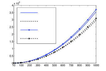
Figure 2: Condition number $\kappa_{\infty}(N)$ and stiffness ratio $\kappa_{A}(N)$ for the benchmark solution II (lines without markers) and III (lines with markers).

Note that the quadratic dependence (47) on the number of nodes $N$ follows from the proportionality of the pressure to the opening accepted in the Nordgren model. In the case when the pressure and the opening are connected by the exact equations of the elasticity theory, the dependence becomes cubic (see, e.g. [2]). For $N=10^{5}$, the stiffness ratio becomes of order $10^{15}$ what is critical for most of the solvers. In this respect, employing iterations in the fluid velocity may be a reasonable strategy despite it requires repeated solving of ODE and accurate evaluation of the velocity after an iteration. Still, using the system (45), (46) looks beneficial in a vicinity of the fluid front in the general case of a 2D fracture. Then the number of nodal points may be taken small enough to avoid too stiff system.

4 Accuracy of computations

We shall use two mentioned approaches for approximation of the spatial derivatives.

The first one, leading to the dynamic system (45), (46), has been suggested and explained when analyzing stiffness. It results in a well-posed initial (Cauchy) problem for the system of ODE what opens the possibility to solve the problem by well-established methods, like those of Runge-Kutta. Making use of this opportunity, we applied the standard MATLAB solver ode15s. It is based on the Runge-Kutta method and employs automatic choice of the time step.

The other option consists in substitution of the velocity, defined by (31), into (30) only for the term $\partial v/\partial\varsigma$. Then the equation contains the propagation speed $V_{\ast}$ and the particle velocity $v$ in the multiplier by the first spatial derivative:

$$\frac{\partial y}{\partial t}=\frac{k_{l}k_{e}}{x_{\ast}^{2}}y\frac{\partial^{2}y}{\partial\varsigma^{2}}+\frac{1}{x_{\ast}}(\varsigma V_{\ast}-v)\frac{\partial y}{\partial\varsigma}-3y^{2/3}q_{l}.$$ (48)

We compliment (48) with the regularized speed equation (36), which after integration in time and accounting for the asymptotics (32) may be written as

$$x_{\ast}^{2}=x_{\ast 0}^{2}+2\frac{k_{l}k_{e}}{3}\int_{t_{0}}^{t}\lim_{\varsigma\rightarrow 1}\frac{y(\varsigma,t)}{1-\varsigma}dt.$$ (49)

This form of equations is convenient for employing an implicit time stepping method, for example, the classical Crank-Nicolson scheme. The boundary conditions on a time step are obtained by using the discretized equations (34) (at the inlet) and (35) (at the $\varepsilon$-regularized opening condition). The resulting non-linear algebraic system is solved by successive iterations. At each of the iterations, we consider a linear system by taking fixed values of $y$, $v$, $V_{\ast}$ and $x_{\ast}$ in the non-linear terms. At an iteration, for fixed coefficients in front of the spatial derivatives and leak-off term and for fixed coefficients in non-linear boundary conditions, the algebraic system is tri-diagonal. It is efficiently solved by the sweep-method. At the end of an iteration, we obtain new nodal values of $y$, which serve to evaluate new values of $V_{\ast}$ and $v$ by using (31), and new value of $x_{\ast}$ by using (49). The non-linear terms are iterated within a time step until the difference of values obtained on successive iterations becomes less than a prescribed tolerance. For a sufficiently small time step, the values obtained on the previous time step may serve as acceptable approximations, then one iteration is usually sufficient to meet the tolerance.

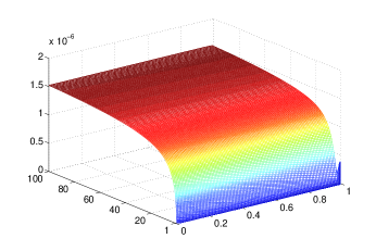
Figure 3: Relative error of the crack opening for the benchmark solution II: a) computations by Runge-Kutta method for the system (45), (46) after spatial discretization, b) computations by Crank-Nicolson method for the system (48), (49) after temporal and spatial discretization.

We compare the accuracy of the solution, obtained by the standard Runge-Kutta MATLAB solver ode15s for the dynamic system, with that, obtained by the Crank-Nicolson method with iterations on a time step for the discretized system (48), (49) and discretized boundary conditions (34) and (35). In both cases, we used the same second order approximations for the first and second spatial derivatives. The number $N$ of nodal points uniformly spaced on the interval $[0,1-\varepsilon]$ and the regularization parameter $\varepsilon$, were also the same: $N=100$ and $\varepsilon=10^{-4}$. Time stepping in the second approach was taken similar to that generated by the solver ode15s for solving the dynamic system of the first approach. The time interval $[1,100]$ was also the same for both approaches. Thus the conditions for the comparison were practically the same. Fig. 3 illustrates the comparative accuracy of the two approaches. It presents the relative error $\delta w$ of the opening obtained by the first (Fig. 3a) and the second (Fig. 3b) approaches for the benchmark solution II. We see that the both approaches provide high accuracy: the relative error does not exceed $1.8\cdot 10^{-6}$. Still, the Crank-Nicolson scheme provides two-order less error ($\delta w<10^{-8}$), except for the time close to the initial moment ($t_{0}=1$) and nodes closest to the crack tip ($\varsigma=1$). (Surely, the error of the approach, using the Crank-Nicolson scheme, for small time and near the tip, may be decreased to the level $10^{-8}$, as well, by decreasing the first time steps and increasing the number of iterations within a time step).

The Crank-Nicolson scheme served us also to compare the accuracy of results, obtained by using (i) the SE (49), and (ii) the global mass balance. In the normalized variables, the latter has the form:

$$x_{\ast}(t)\int_{0}^{1}w(\varsigma,t)d\varsigma=x_{\ast}(t_{0})\int_{0}^{1}w(\varsigma,t_{0})d\varsigma+\int_{t_{0}}^{t}q_{0}(t)dt-\int_{t_{0}}^{t}x_{\ast}(t)\int_{0}^{1}q_{l}(\varsigma,t)d\varsigma dt.$$

The calculations show that, when employing the global mass balance, the maximal relative error $\delta w$ of the opening becomes $1.4\cdot 10^{-3}$. It is three-order greater than the error, obtained when employing the SE. This can be explained by an additional error induced by numerical integration over the interval [0,1]. This implies that using the local SE instead of the global mass balance is beneficial for the accuracy even in 1D problems.

Finally we analyze the dependence of the accuracy on the distribution of the fluid velocity along the fracture. Table 1 presents the maximal relative error  of the opening $\delta w$ and the fracture length $\delta x_{\ast}$ for the benchmark solutions I, II and III. The data are obtained by using the first approach. The second line of the table contains the maximal relative variation $\gamma_{v}$ of the fluid velocity. It can be seen that the variation notably influences the accuracy. Even in the cases of the benchmark solutions I and II, when the variation $\gamma_{v}$ is of the same order, there is significant (an order) difference in the accuracy. For strongly non-uniform distribution, corresponding to the benchmark solution III, the relative error is three orders greater than that for the most uniform distribution, corresponding to the benchmark solution II. This implies that numerical modeling of fractures with notable variations of the fluid velocity requires tests with growing density of the spatial mesh.

	$benchmark\,I$	$benchmark\,II$	$benchmark\,III$
$\gamma_{v}$	0.06	0.02	0.4
$\delta w$	$4.86\cdot 10^{-5}$	$1.54\cdot 10^{-6}$	$5.04\cdot 10^{-3}$
$\delta x_{*}$	$7.23\cdot 10^{-5}$	$1.97\cdot 10^{-6}$	$6.84\cdot 10^{-3}$

Table 1: Accuracy of the crack opening $\delta w$ and crack length $\delta x_{*}$ for various benchmark solutions.

5 Sensitivity analysis

For zero leak-off, the only parameter, defining the solution, is the influx at the inlet $q_{0}$. Consider its perturbed value $q_{0}+\Delta q_{0}$, so that the relative change of the influx is $\delta q_{0}=\Delta q_{0}/q_{0}$. We are interested in finding relative changes of the opening $\delta w=\Delta w/w$, the pressure $\delta p=\Delta p/p$, the fracture length $\delta x_{*}=\Delta x_{\ast}/x_{\ast}$, the particle velocity $\delta v=\Delta v/v$ and the front speed $\delta V=\Delta V_{\ast}/V_{\ast}$. From the analytical solution (38), (39), we easily obtain:

$${\delta w}=\delta p=(1+\delta\xi_{\ast})^{2/3}-1,\quad\delta v=\delta V_{\ast}=\delta x_{\ast}=\delta\xi_{\ast}.$$

In Sec. 2, it was stated that $\xi_{\ast}$ is proportional to $q_{0}^{3/5}$. Hence, $1+\delta\xi_{\ast}=(1+\delta q_{0})^{3/5}$, and finally the relative changes are:

$$\delta w=\delta p=(1+\delta q_{0})^{2/5}-1,\quad\delta v=\delta V_{\ast}=\delta x_{\ast}=(1+\delta q_{0})^{3/5}-1.$$

For a small relative change of the influx, to the accuracy of terms of order $O\left(\delta q_{0}^{3}\right)$, we have:

$$\delta w=\delta p=0.4\delta q_{0}-0.12\delta q_{0}^{2},\quad\delta v=\delta V_{\ast}=\delta x_{\ast}=0.6\delta q_{0}-0.12\delta q_{0}^{2}.$$ (50)

This implies that the relative changes equal approximately to one-half of the relative change of the influx. Note that the disturbances of the solution change its sign when $\delta q_{0}$ changes the sign.

In cases, when the disturbance $\delta q_{0}$ oscillates in time with the amplitude $A$ and the angular frequency $\omega_{q}$ as $\delta q_{0}=A\sin(\omega_{q}(t-t_{0}))$, we may numerically evaluate its influence on the solution by employing any of the discussed approaches. The results, obtained when solving the discretized dynamic system (45), (46) by using standard MATLAB solver ode15s are presented in Fig. 4.

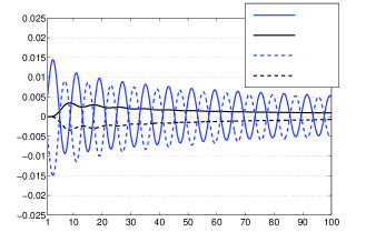
Figure 4: Relative fluctuations of the crack opening $\delta w_{0}$ and the crack length $\delta x_{*}$, caused by the periodic disturbance of the influx: a) benchmark solution II, b) benchmark solution III.

The graphs are plotted for the relative amplitude of perturbation $A/q_{0}=\pm 0.1$ and $\omega_{q}=\pi/4$. They present the relative fluctuations of the crack opening, $\delta w_{0}=\Delta w(0,t)/w(0,t)$, at the inlet point ($\varsigma=0$) and relative fracture length $\delta x_{\ast}$ in time for the benchmark solution II (Fig. 4a) and III (Fig. 4b). Solid lines refer to the case when $A/q_{0}=+0.1$, dashed lines to $A/q_{0}=-0.1$. It can be seen that for the periodic perturbations the crack opening $\delta w_{0}$ is an order less than the amplitude $A$ of the perturbation $\delta q_{0}$ itself, while the position of the crack, $\delta x_{*}$, is two orders less. It is worth noting that the fluctuations depend on the sign of the amplitude $A$, and the change of the fracture length tends to a constant value with growing time. It can be seen that, when the amplitude $A$ changes its sign, the limit of the fluctuation of the fracture length for small leak-off (benchmark II) also changes its sign, while for the large leak-off (benchmark III) the sign is the same.

6 Conclusions

The results presented show that the modified formulation of the problem [19] – [22], employing the suggested variables, speed equation and $\varepsilon$-regularization, extends the opportunities for better numerical modeling of the hydraulic fracture propagation. Specifically, the improvements may include:

(i) drastic decrease of stiffness of ODE, obtained after spatial discretization, by employing iterations in the particle velocity;

(ii) avoiding iterations in non-linear terms and using highly efficient standard solvers by including the SE into the system of ODE as suggested in Sec. 3;

(iii) increasing the accuracy of time-stepping schemes of Crank-Nicolson type by using the SE instead of the commonly used global mass balance.

The advantages of the modified formulation have been illustrated by considering the simplest 1D problem by Nordgren. Meanwhile, the suggested formulation and approaches, being general, they are applicable to 2D fractures. They are of special interest for modeling the area behind the fluid front, where gradients of the pressure and opening are high.

Acknowledgements

This research has been supported by FP7 Marie Curie IAPP project (PIAP-GA-2009-251475). MW and AM are grateful respectively to the Institute of Mathematics and Physics of Aberystwyth University and EUROTECH for the facilities and hospitality.

References

- [1] Adachi, J., Detournay, E. 2002. Self-similar solution of a plane-strain fracture driven by a power-law fluid. Int. J. Numer. Anal. Methods Geomech. 26, 579–604.
- [2] Adachi, J., Siebrits E., Peirce A., Desroches J. 2007. Computer Simulation of Hydraulic Fractures. International Journal of Rock Mechanics and Mining Sciences, 44, 739-757.
- [3] Bunger, A.P., Detournay, E. & Garagash, D.I. 2005. Toughness-dominated hydraulic fracture with leak-off. Int. J. Fracture, 134, 175-190.
- [4] Carter, E. 1957. Optimum fluid characteristics for fracture extension. In: Howard, G., Fast, C. (eds.) Drilling and Production Practices, pp. 261–270. American Petroleum Institute.
- [5] Desroches, J., Detournay, E., Lenoach, B., Papanastasiou, P., Pearson, J., Thiercelin, M., Cheng, A.-D. 1994. The crack tip region in hydraulic fracturing. Proc. Roy. Soc. Lond. Ser. A 447, 39–48 (1994)
- [6] Detournay, E. 2004. Propagation regimes of fluid-driven fractures in impermeable rocks. Int. J. Geomech. 4(1), 1–11.
- [7] Economides, M., Nolte, K. (eds.). 2000. Reservoir Stimulation. 3rd edn. Wiley, Chichester, UK.
- [8] Garagash, D. I. 2006. Propagation of a plane-strain hydraulic fracture with a fluid lag: Early time solution. Int. J. Solids Struct. 43, 5811-5835.
- [9] Garagash, D., Detournay, E. 2000. The tip region of a fluid-driven fracture in an elastic medium. ASME J. Appl. Mech. 67(1), 183–192 (2000).
- [10] Garagash, D.I., Detournay, E. & Adachi, J. I. 2011. Multiscale tip asymptotics in hydraulic fracture with leak-off. J. Fluid Mech., 669, 260-297.
- [11] Geertsma, J. & de Klerk, F. 1969. A rapid method of predicting width and extent of hydraulically induced fractures. J. Pet. Tech., 21, 1571-1581.
- [12] Hadamard, J. 1902. Sur les problemes aux derivees partielles et leur signification physique. Princeton University Bulletin, 49-52.
- [13] Higham, N. 1986. Efficient algorithms for computing the condition number of a tridiagonal matrix. The University of Manchester, MIMS EPrint 2007.8.
- [14] Howard, G.C. & Fast, C.R. 1970. Hydraulic fracturing. Monograph Series Soc. Petrol. Eng., Dallas.
- [15] Hu, J. & Garagash, D.I. (2010). Plane strain propagation of a fluid-driven crack in a permeable rock with fracture toughness. ASCE J. Eng. Mech., 136, 1152-1166.
- [16] Jamamoto, K. & Shimamoto, T. & Sukemura, S. 2004. Multi fracture propagation model for a three-dimensional hydraulic fracture simulator. Int. J. Geomech. ASCE, 1, 46-57.
- [17] Kovalyshen, Y. and Detournay, E. 2009. A reexamination of the classical PKN model of hydraulic fracture, Transp Porous Med, 81, 317-339.
- [18] Khristianovich, S.A. & Zheltov, V.P. 1955. Formation of vertical fractures by means of highly viscous liquid. In: Proc. 4-th World Petroleum Congress, Rome, 579-586.
- [19] Linkov, A.M. 2011. Speed equation and its application for solving ill-posed problems of hydraulic fracturing. ISSM 1028-3358, Doklady Physics, Vol.56, No.8, pp.436-438. Pleiades Publishing, Ltd. 2011.
- [20] Linkov, A.M. Use of a speed equation for numerical simulation of hydraulic fractures. Available at: http://arxiv.org/abs/1108.6146. Date: Wed, 31 Aug 2011 07:47:52 GMT (726kb). Cite as: arXiv: 1108.6146v1 [physics.flu-dyn].
- [21] Linkov, A.M. 2011. On numerical simulation of hydraulic fracturing. Proc. XXXVIII Summer School-Conference, “Advanced Problems in Mechanics-2011”, Repino, St. Petersburg, July 1-5, 2011, 291-296.
- [22] Linkov, A.M. 2012. On efficient simulation of hydfraulic fracturing in terms of particle velocity. Int. J. Eng. Sci., 52, 77-88.
- [23] Mitchell, S.L., Kuske, R., Peirce, A. 2007. An asymptotic framework for finite hydraulic fractures including leakoff. SIAM J. Appl. Math. 67(2), 364–386.
- [24] Nolte, K.G. (1988). Fracture design based on pressure analysis. Soc. Pet. Eng. J., Paper SPE 10911, February, 1-20.
- [25] Nordgren R.P. 1972. Propagation of a Vertical Hydraulic Fracture. J. Pet. Tech, 253, 306-314.
- [26] Perkins, T., Kern, L. 1961. Widths of hydraulic fractures. J. Pet. Tech. Trans. AIME 222, 937–949.
- [27] Savitski, A. & Detournay, E. 2002. Propagation of a fluid driven penny-shaped fracture in an impermeable rock: asymptotic solutions. Int. J. Solids Struct. 39, 6311-6337.
- [28] Sethian, J.A. 1999. Level set methods and fast marching methods. Cambridge, Cambridge University Press.
- [29] Spence, D.A., Sharp P. W. 1985. Self-similar solutions for elastohydrodynamic cavity flow. Proc. Roy. Soc. London, Series A, 400, 289-313.