Abundances of neutron-capture elements in G 24-25

Abstract

Aims. The differences between the neutron-capture element abundances of halo stars are important to our understanding of the nucleosynthesis of elements heavier than the iron group. We present a detailed abundance analysis of carbon and twelve neutron-capture elements from Sr up to Pb for a peculiar halo star G 24-25 with [Fe/H] = $-1.4$ in order to probe its origin.

Methods. The equivalent widths of unblended lines are measured from high resolution NOT/FIES spectra and used to derive abundances based on Kurucz model atmospheres. In the case of CH, Pr, Eu, Gd, and Pb lines, the abundances are derived by fitting synthetic profiles to the observed spectra. Abundance analyses are performed both relative to the Sun and to a normal halo star G 16-20 that has similar stellar parameters as G 24-25.

Results. We find that G 24-25 is a halo subgiant star with an unseen component. It has large overabundances of carbon and heavy $s$-process elements and mild overabundances of Eu and light $s$-process elements. This abundance distribution is consistent with that of a typical CH giant. The abundance pattern can be explained by mass transfer from a former asymptotic giant branch component, which is now a white dwarf.

1 Introduction

The heaviest elements in halo stars are mainly produced by neutron captures divided into the slow ($s$-) and the rapid ($r$-) processes, which have different reaction timescales. Among the $s$-process synthesized elements, lead (Pb) is particularly interesting because it is the most abundant element in the third peak of the nuclei distribution in stars. However, Pb lines are very weak in low metallicity stars, and thus Pb abundances have not been measured for many stars compared with other $s$-process elements, such as Ba. Pb is often detected for carbon-enhanced stars with enhanced Ba abundances. For example, Bisterzo et al. (2006) compiled a catalog of 23 Pb-rich stars found in the literature. Most of these stars have [Fe/H] $<-2$ and are carbon-enhanced metal-poor stars with $s$-process enhanced abundances (CEMP-$s$) or with $r$- and $s$-process enhanced abundances (CEMP-$r/s$). Eleven stars of the CEMP-$s$/CEMP-$r/s$ compiled in Bisterzo’s work are proven members of binary systems (McClure & Woodsworth 1990; Aoki et al. 2001, 2002b; Lucatello et al. 2003; Cohen et al. 2003; Sivarani et al. 2004).

In the past ten years, some studies also reported Pb measurements for Ba stars and CH giants and subgiants (Van Eck et al. 2001, 2003; Johnson & Bolte 2004; Allen & Barbuy 2006; Pereira & Drake 2009, 2011; Goswami & Aoki 2010).These classes of stars exhibit overabundances of $s$-process elements; in addition, the CH stars have high C abundances. Furthermore, these stars fall into different metallicity ranges and belong to different populations in the Galaxy. Most of the Ba stars are found in the disk with [Fe/H] from $-$0.5 to +0.4; fewer than 6$\%$ of the Ba stars belong to the halo (Mennessier et al. 1997; Allen & Barbuy 2006). The classical CH giants are clearly members of the halo population with $-1.5<$[Fe/H]$<-1.0$ (Vanture 1992a). The CH subgiants, i.e stars with similar abundance distributions as the CH giants, but situated on either the main sequence or the subgiant branch, have typical [Fe/H] values in the range from $-0.5$ to $-0.2$ and disk population kinematics (Luck & Bond 1982, 1991; Sneden & Parthasarathy 1983; Smith et al. 1993).

Systematic spectroscopic studies indicate that all Ba and CH stars belong to binary systems (McClure & Woodsworth 1990). At low metallicity, [Fe/H]$<-1.8$, Lucatello et al. (2005) found that 68$\%$ of 19 CEMP-$s$ stars display evidence of radial velocity variations. This high frequency suggests that all CEMP-s stars are metal-poor analogs of the classical CH giants. The origin of the enhanced carbon and $s$-process elements (including Pb) in these stars could be explained by mass transfer from a former asymptotic giant branch (AGB) companion (now a white dwarf) in a binary system.

In a study of two distinct halo populations in the solar neighborhood, Nissen & Schuster (2010, 2011) measured the abundance ratios and kinematics of 94 dwarf and subgiant stars and found a strong enhancement of [Ba/Fe] for a halo star, G 24-25, with [Fe/H] = $-1.4$. Further investigation of the spectrum identified a Pb line at 4057.8 Å, which is not seen for the rest of the stars. For example, the Pb feature at 4057.8 Å cannot be detected in G 16-20, a halo star with a similar metallicity as G 24-25. In addition, G 24-25 has a strong CH band near 4300 Å, indicating that it is a CH subgiant. To our knowledge, this is the first known CH subgiant with a metallicity that is typical of the halo population. In this paper, we report our abundance measurements of Pb and other neutron-capture elements for this peculiar halo star. For comparison, G 16-20 is analyzed as a reference star. The abundance pattern is compared with other chemically peculiar stars in the literature, and simple AGB wind-accretion models are adopted to reproduce the measured abundances.

2 Abundance analysis

2.1 Observational data and atmospheric parameters

As described in Nissen & Schuster (2010), the spectra of G 24-25 and G 16-20 were obtained at the 2.56m Nordic Optical Telescope (NOT) using the FIbre fed Echelle Spectrograph (FIES) with a resolving power of R $\sim$ 40,000. The spectral range goes from 4000 Å to 7000 Å, and the signal-to-noise ratio ($S/N$) equals about 170 at 5500 Å  but is only between 50 and 80 in the blue spectral region.

The stellar atmospheric parameters for G 24-25 and G 16-20 are taken from Nissen & Schuster (2010) and given in Table 1, where the heliocentric radial velocities are also given. According to Nissen & Schuster (2010), the total space velocities with respect to the local standard of rest are 315 km s^-1 and 263 km s^-1 for G 24-25 and G 16-20, respectively, which clearly classify both stars as members of the halo population.

Table 1: Atmospheric parameters and radial velocities of G 24-25 and G 16-20.

Star	$T_{\mbox{\scriptsize eff}}$	$\log g$	$\mathrm{[Fe/H]}$	$\xi$	$v_{\mbox{\scriptsize rad}}$
	(K)			(km s-1)	(km s-1)
G 24-25	$5828$	$3.86$	$-1.40$	$1.20$	$-312.9$
G 16-20	$5625$	$3.64$	$-1.42$	$1.50$	$\leavevmode\nobreak\ \leavevmode\nobreak\ 170.8$

2

Table 2: Atomic data and equivalent widths of spectral lines, as well as the derived abundances for G 24-25 and G 16-20. This table contains the following information: wavelength in angstroms (Column 1), element identification (Column 2), excitation potential (Column 3), log of the oscillator strength (Column 4), reference for log gf (Column 5), measured equivalent width in milli-angstroms and derived abundance of G 24-25 (Columns 6 and 7), measured equivalent width in milli-angstroms and derived abundance of G 16-20 (Columns 8 and 9).

Wavelength	Elem.	E. P.	log gf	Ref.	G 24-25			G 16-20
(Å)		(eV)			$EW$ (mÅ)	log $\varepsilon$		$EW$ (mÅ)	log $\varepsilon$
4932.049	C i	7.68	$-1.68$	1	14.6	8.08		…	…
5052.167	C i	7.68	$-1.30$	1	23.8	7.97		1.2:	6.58:
5380.337	C i	7.68	$-1.62$	1	14.1	8.02		…	…
4607.340	Sr i	0.00	$0.28$	2	18.0	1.96		5.7	1.19
4077.714	Sr ii	0.00	$0.17$	2	234.8	1.79		154.3	1.09
4398.010	Y ii	0.13	$-1.00$	3	50.9	1.58		18.3	0.56
4883.690	Y ii	1.08	$0.07$	3	56.1	1.52		25.0	0.60
4900.110	Y ii	1.03	$-0.09$	3	56.2	1.63		23.5	0.67
5087.430	Y ii	1.08	$-0.17$	3	43.4	1.45		15.0	0.54
5123.220	Y ii	0.99	$-0.83$	3	22.0	1.51		4.5	0.53
5200.420	Y ii	0.99	$-0.57$	3	30.8	1.46		8.8	0.58
5205.730	Y ii	1.03	$-0.34$	3	39.3	1.47		14.7	0.64
5402.780	Y ii	1.84	$-0.44$	3	8.6	1.44		…	…
4687.800	Zr i	0.73	$0.55$	4	4.7	2.14		…	…
4050.330	Zr ii	0.71	$-1.06$	5	23.2	2.06		11.5	1.47
4090.510	Zr ii	0.76	$-1.01$	6	26.7	2.14		…	…
4161.200	Zr ii	0.71	$-0.59$	5	46.7	2.15		24.1	1.39
4208.990	Zr ii	0.71	$-0.51$	5	47.0	2.07		26.1	1.36
4258.050	Zr ii	0.56	$-1.20$	5	27.2	2.13		…	…
5350.080	Zr ii	1.83	$-1.24$	6	2.9	2.20		…	…
5350.310	Zr ii	1.77	$-1.16$	5	4.2	2.22		…	…
5853.688	Ba ii	0.60	$-0.91$	7	94.6	2.15		29.5	0.55
6141.727	Ba ii	0.70	$-0.03$	7	163.1	2.08		69.0	0.53
6496.908	Ba ii	0.60	$-0.41$	7	142.5	2.13		61.6	0.64
4526.110	La ii	0.77	$-0.59$	8	15.0	1.22		…	…
4662.510	La ii	0.00	$-1.24$	8	22.8	1.28		…	…
4748.730	La ii	0.93	$-0.54$	8	14.7	1.23		…	…
4920.960	La ii	0.13	$-0.58$	8	48.8	1.38		10.1	0.06
4921.780	La ii	0.24	$-0.45$	8	45.2	1.27		10.6	0.07
4053.490	Ce ii	0.00	$-0.61$	9	29.5	1.71		…	…
4062.230	Ce ii	1.37	$0.30$	10	19.6	1.88		1.2:	0.36:
4083.220	Ce ii	0.70	$0.27$	9	36.1	1.70		…	…
4117.290	Ce ii	0.74	$-0.45$	9	11.3	1.69		…	…
4118.140	Ce ii	0.70	$0.13$	9	32.4	1.74		…	…
4120.830	Ce ii	0.32	$-0.37$	9	31.9	1.85		…	…
4127.360	Ce ii	0.68	$0.31$	9	40.9	1.76		…	…
4153.130	Ce ii	0.23	$-0.80$	9	16.7	1.74		…	…
4222.600	Ce ii	0.12	$-0.15$	9	46.6	1.80		6.6	0.28
4427.920	Ce ii	0.54	$-0.41$	9	19.2	1.71		…	…
4460.230	Ce ii	0.47	$0.28$	10	…	…		10.7	0.41
4483.900	Ce ii	0.86	$0.10$	9	29.0	1.79		…	…
4523.080	Ce ii	0.52	$-0.08$	9	…	…		3.1	0.24
4539.740	Ce ii	0.33	$-0.08$	9	42.5	1.78		5.4	0.30
4560.960	Ce ii	0.68	$-0.26$	9	23.5	1.82		…	…
4562.360	Ce ii	0.48	$0.21$	9	50.6	1.85		7.0	0.29
4565.840	Ce ii	1.09	$0.07$	9	18.2	1.74		…	…
4628.160	Ce ii	0.52	$0.14$	9	46.1	1.83		…	…
5044.030	Ce ii	1.21	$-0.14$	9	10.4	1.72		…	…
5187.450	Ce ii	1.21	$0.17$	9	18.1	1.71		…	…
5274.230	Ce ii	1.04	$0.13$	9	23.3	1.72		…	…
5330.540	Ce ii	0.87	$-0.40$	9	12.4	1.72		…	…
5468.380	Ce ii	1.40	$-0.07$	9	8.9	1.75		…	…
5610.246	Ce ii	1.05	$-0.74$	10	6.0	1.85		…	…
5322.800	Pr ii	0.48	$-0.32$	11	syn	1.28		syn	$<-0.38$
4012.700	Nd ii	0.00	$-0.74$	12	27.0	1.56		4.3	0.35
4051.150	Nd ii	0.38	$-0.30$	13	28.5	1.54		6.4	0.48
4232.380	Nd ii	0.06	$-0.47$	13	35.1	1.53		…	…
4542.603	Nd ii	0.74	$-0.28$	13	17.2	1.49		2.4	0.34
4645.770	Nd ii	0.56	$-0.76$	13	10.0	1.49		…	…
5089.830	Nd ii	0.28	$-1.40$	2	5.5	1.53		…	…
5092.780	Nd ii	0.30	$-0.61$	13	21.4	1.46		2.6	0.29
5192.620	Nd ii	1.14	$0.27$	13	25.6	1.53		3.6	0.33
5234.210	Nd ii	0.55	$-0.51$	13	21.2	1.59		…	…
5249.600	Nd ii	0.98	$0.20$	13	26.9	1.47		…	…
5255.510	Nd ii	0.20	$-0.67$	13	25.8	1.53		…	…
5311.480	Nd ii	0.99	$-0.42$	13	8.3	1.44		…	…
5319.820	Nd ii	0.55	$-0.21$	12	31.1	1.55		3.6	0.20
5385.890	Nd ii	0.74	$-0.82$	12	7.6	1.54		…	…
4244.700	Sm ii	0.28	$-0.73$	14	10.1	0.93		…	…
4434.320	Sm ii	0.38	$-0.26$	15	24.6	1.06		4.6	$-0.04$
4458.520	Sm ii	0.10	$-0.78$	15	14.3	0.97		…	…
4519.630	Sm ii	0.54	$-0.43$	14	14.8	1.07		…	…
4523.910	Sm ii	0.43	$-0.58$	14	13.7	1.06		…	…
4566.210	Sm ii	0.33	$-0.92$	15	9.6	1.11		…	…
4642.230	Sm ii	0.38	$-0.52$	14	12.1	0.93		2.4	$-0.09$
4674.600	Sm ii	0.18	$-0.56$	15	15.6	0.90		3.7	$-0.07$
4687.180	Sm ii	0.04	$-1.17$	15	9.7	1.07		…	…
4129.700	Eu ii	0.00	$0.22$	16	syn	$-0.25$		syn	$-0.50$
6645.130	Eu ii	1.38	$0.20$	16	syn	$-0.30:$		syn	$-0.56$:
4191.080	Gd ii	0.43	$-0.48$	17	syn	0.84		syn	0.08:
4057.810	Pb i	1.32	$-0.22$	18	syn	2.28		syn	$<0.60$
References to Table LABEL:Tab:EWandloggf $-$ (1) Hibbert et al. (1993); (2) Gratton & Sneden (1994);
(3) Hannaford et al. (1982); (4) Biémont et al. (1981); (5) Ljung et al. (2006);
(6) Cowley & Corliss (1983); (7) Davidson et al. (1992); (8) Lawler et al. (2001);
(9) Lawler et al. (2009); (10) Palmeri et al. (2000); (11) Mashonkina et al. (2009);
(12) Meggers et al. (1975); (13) Den Hartog et al. (2003); (14) Biémont et al. (1989);
(15) Corliss & Bozman (1962); (16) Mashonkina & Gehren (2000);
(17) Den Hartog et al. (2006); (18) Biémont et al. (2000).

Table 2: continued.

2.2 Line selection and atomic data

The atomic lines were selected from previous abundance determinations of the heavy elements of stars, namely Sneden & Parthasarathy (1983), Gratton & Sneden (1994), Sneden et al. (1996), Reddy et al. (1997), Aoki et al. (2001, 2002b), Cowan et al. (2002), Sivarani et al. (2004), and Johnson & Bolte (2004). The log gf values are primarily adopted from high-precision laboratory measurements; references are given in Table LABEL:Tab:EWandloggf.

2.3 Abundance calculations

For most elements, the abundances are derived from equivalent widths (EWs) of unblended lines measured by fitting a Gaussian to the line profile. For blended lines and/or lines with significant hyperfine structure (HFS) and/or isotope splitting, the abundances are derived by spectrum synthesis. The model atmospheres of Kurucz, (1993) are used, and local thermodynamic equilibrium (LTE) is assumed.

The carbon abundance is derived from the $EW$s of three unblended C i atomic lines providing [C/Fe] = 1.03 and [C/Fe] = $-$0.39 for G 24-25 and G 16-20, respectively. Compared to G 16-20, G 24-25 has clear carbon atomic lines and strong CH and C₂ lines. From spectrum synthesis fitting of the CH A-X band of G 24-25 around 4310 Å (Fig. 1), we obtained [C/Fe] = 1.05 when using the CH molecular line data of Barklem et al. (2005). The abundances derived from the C i atomic lines and the CH A-X band are consistent, whereas Sivarani et al. (2004) reported that carbon abundances derived from C i lines are on average about 0.1-0.3 dex higher than those obtained from the CH lines.

Figure 1: The CH feature near 4310 Å. The observed spectrum of G 24-25 is shown as bold dots. The solid line shows the synthetic spectrum corresponding to [C/Fe] = 1.05. The dot-dashed and dashed lines, corresponding to $\Delta$[C/Fe] = $\pm$0.07, are shown to illustrate the sensitivity of line strengths to variations in the carbon abundance.

Since the CN 3800 Å band is not covered in our spectra, we tried to derive the nitrogen abundance by spectrum synthesis fitting of the CN 4215 Å band adopting molecular line data from Aoki et al. (2002a). The CN lines around 4215 Å are quite weak ($EW<5$ mÅ), and due to the rather low $S/N$ ratio in this spectral region, we can only get an upper limit [N/Fe] $<0.16$ dex for G 24-25. In the case of G 16-20 we get [N/Fe] $<0.0$ dex.

The abundances of the light $s$-process elements Sr, Y, and Zr, as well as the heavy neutron-capture elements Ba, La, Ce, Nd, and Sm are derived from EW measurements, whereas spectrum synthesis is used for Pr, Eu, Gd, and Pb. The HFS of the Ba ii lines at 5853.7, 6141.7, and 6496.9 Å is not taken into account since it is insignificant according to Sneden et al. (1996) and Mashonkina et al. (2010). Our Ba abundances are in good agreement with those in Nissen & Schuster (2011), who also found that the effects of HFS on the Ba lines are negligible. The La ii and Sm ii lines are quite weak, and we do not include any HFS.

The collisional broadening of lines induced by neutral hydrogen is also considered. The width cross-sections of the C i, Sr i, Sr ii, and Ba ii lines are taken from Anstee & O’Mara (1995), Barklem & O’Mara (1997, 2000), and Barklem et al. (2000). For the remaining lines, we follow Cohen et al. (2003) and adopt the Unsöld (1955) approximation to the van der Waals interaction constant enhanced by a factor of two. For the four strong lines, Sr ii 4077.7 Å and the Ba ii lines at 5853.7, 6141.7, and 6496.9 Å, the effect on the derived abundances of the uncertainties in the damping constants is approximately 0.08 dex. However, most element abundances in our work are based on weak lines ($EW<60$ mÅ), for which the influence on the results caused by the uncertainties in the collisional cross-sections is negligible. Hence, we do not discuss possible errors in the damping constants in Sect. 2.4.

The spectrum synthesis fits to the Pr, Eu, and Gd lines are shown in Fig. 2. The atomic and hyperfine structure data for the Pr i 5322.8 Å and Eu ii 4129.7 Å lines are adopted from Mashonkina et al. (2009) and Mashonkina & Gehren (2000), respectively. The log gf value for the Gd ii line at 4191.1 Å is taken from Den Hartog et al. (2006).

Figure 2: Comparison of observed (bold dots) and synthetic profiles of the spectral lines of the heavy elements Pr (top panel), Eu (middle), and Gd (bottom). The respective elemental abundances corresponding to the full drawn lines are listed in Table 5. Two alternative synthetic spectra are shown to demonstrate the sensitivity of the line strength to the abundance.

In the observed spectrum of G 24-25, we could detect one lead line, the Pb i $\lambda 4057.8$, which is too weak to be seen in the spectrum of G 16-20 (Fig. 3). The log gf value is taken from Biémont et al. (2000) and the hyperfine data are taken from Aoki et al. (2001). Compared to G 16-20, a more normal neutron-capture star, it is clear that G 24-25 exhibits a strong Pb line. The spectral region from 4057.6 Å to 4058 Å does not show a smooth line profile for G 24-25, but considering that the estimated $S/N$ around the Pb line is only about 60, we propose that this is probably due to noise. Thus, a $\chi^{2}$ fitting of the ten observed data points from 4057.69 Å to 4057.92 Å was applied to determine the lead abundance. The $\chi^{2}$ was computed as described by Nissen et al. (1999), i.e.

$$\ \rm\chi^{2}=\frac{\sum(O_{i}-S_{i})^{2}}{\sigma^{2}},$$

where $O_{i}$ is the observed relative flux, $S_{i}$ the synthetic flux, and $\sigma$ = $(S/N)^{-1}$ = 1/60. The value of [Pb/Fe] was varied in steps of 0.02 dex to find the lowest $\chi^{2}$. The result is a parabolic variation in $\chi^{2}$ as shown in Fig. 4. The most probable value of [Pb/Fe] corresponds to the minimum of $\chi^{2}$, and $\Delta\chi^{2}$ = 1, 4, and 9 (the dashed horizontal lines) correspond to the 1-,2-, and 3-$\sigma$ confidence limits of determining exclusively [Pb/Fe]. The spectrum synthesis fit to the Pb line for the abundance corresponding to the minimum $\chi^{2}$ ([Pb/Fe] = 1.68) is shown as the solid line in Fig. 3. A Gaussian broadening function was applied to fit the observed spectrum in order to take the combined effect of instrumental, macro-turbulent, and rotational broadening into account. The nearby spectral lines could be well-fitted in this way leading to a FWHM of the Gaussian function of $7.8\pm 1$ km s^-1. The corresponding uncertainty in [Pb/Fe] is around 0.04 dex.

Figure 3: Spectrum-synthesis fitting of the Pb I $\lambda 4057.81$ line for G 16-20 and G 24-25.

Figure 4: The $\chi^{2}$ variation in the synthetic fit to ten observed data points from 4057.69 Å to 4057.92 Å applied to the determination of the lead abundance in G 24-25.

2.4 Error analysis

The uncertainties in the abundances arise from random and systematic errors. The random errors associated with the errors in the log gf values and the EW measurements can be estimated from the line-to-line scatter in the abundances of a given element, based on many lines. The random error in the mean abundance is ${\sigma}_{\rm EW}/{\sqrt{N}}$, where $N$ is the number of lines studied. For the elements that have only one line, we use three times the uncertainty given by Cayrel (1988) by taking into consideration the error in the continuum rectification. For instance, Sr i 4607.34 Å with $S/N$ = 130 leads to an error of 0.6 mÅ by using the formula (Eq. 7) given by Cayrel (1988). We then estimate that the error in the EW measurement is 1.8 mÅ for Sr i 4607.34 Å, which results in an error of 0.06 dex in the Sr i abundance calculation.

A significant contribution to the systematic errors comes from the uncertainties in the stellar atmospheric parameters adopted in the abundance determination. This was estimated by varying the model parameters with $\Delta T_{\mbox{\scriptsize eff}}$ = 100 K, $\Delta$ log$g$ = 0.10 dex, $\Delta$[Fe/H] = 0.1 dex, and $\Delta\xi$ = 0.30 km s^-1. The corresponding abundance uncertainties are listed in Tables 3 and 4, and the total uncertainty for each element is estimated by the quadratic sum of the atmospheric and random errors.

An additional systematic error in the derived abundances relative to the solar abundances is introduced by our LTE assumption and the use of one-dimensional model atmospheres. These errors tend, however, to cancel for the abundances of G 24-25 relative to G 16-20, because the two stars have similar atmospheric parameters and also comparable abundances of Fe and the $\alpha$-capture elements.

Table 3: Abundance uncertainties for neutron-capture elements in G 24-25.

Elem.	$\Delta T$	$\Delta\log g$	$\Delta$ [Fe/H]	$\Delta\xi$	$\frac{\sigma_{\rm EW}}{\sqrt{N}}$	$\sigma_{tot}$
	$+100$ K	$+0.10$	$+0.10$	$+0.30$
C i	$-0.06$	$\leavevmode\nobreak\ \leavevmode\nobreak\ 0.03$	$-0.01$	$-0.01$	0.03	0.07
Sr i	$\leavevmode\nobreak\ \leavevmode\nobreak\ 0.08$	$\leavevmode\nobreak\ \leavevmode\nobreak\ 0.00$	$\leavevmode\nobreak\ \leavevmode\nobreak\ 0.01$	$-0.02$	0.06	0.10
Sr ii	$\leavevmode\nobreak\ \leavevmode\nobreak\ 0.06$	$\leavevmode\nobreak\ \leavevmode\nobreak\ 0.01$	$\leavevmode\nobreak\ \leavevmode\nobreak\ 0.03$	$-0.02$	0.04	0.08
Y ii	$\leavevmode\nobreak\ \leavevmode\nobreak\ 0.05$	$\leavevmode\nobreak\ \leavevmode\nobreak\ 0.03$	$\leavevmode\nobreak\ \leavevmode\nobreak\ 0.00$	$-0.06$	0.02	0.09
Zr i	$\leavevmode\nobreak\ \leavevmode\nobreak\ 0.08$	$\leavevmode\nobreak\ \leavevmode\nobreak\ 0.00$	$\leavevmode\nobreak\ \leavevmode\nobreak\ 0.00$	$-0.01$	0.07	0.11
Zr ii	$\leavevmode\nobreak\ \leavevmode\nobreak\ 0.04$	$\leavevmode\nobreak\ \leavevmode\nobreak\ 0.04$	$\leavevmode\nobreak\ \leavevmode\nobreak\ 0.00$	$-0.04$	0.02	0.07
Ba ii	$\leavevmode\nobreak\ \leavevmode\nobreak\ 0.09$	$-0.02$	$\leavevmode\nobreak\ \leavevmode\nobreak\ 0.01$	$-0.10$	0.02	0.14
La ii	$\leavevmode\nobreak\ \leavevmode\nobreak\ 0.05$	$\leavevmode\nobreak\ \leavevmode\nobreak\ 0.02$	$\leavevmode\nobreak\ \leavevmode\nobreak\ 0.00$	$-0.06$	0.03	0.08
Ce ii	$\leavevmode\nobreak\ \leavevmode\nobreak\ 0.05$	$\leavevmode\nobreak\ \leavevmode\nobreak\ 0.03$	$\leavevmode\nobreak\ \leavevmode\nobreak\ 0.00$	$-0.05$	0.01	0.08
Pr ii	$\leavevmode\nobreak\ \leavevmode\nobreak\ 0.04$	$\leavevmode\nobreak\ \leavevmode\nobreak\ 0.04$	$-0.02$	$-0.03$	0.09	0.11
Nd ii	$\leavevmode\nobreak\ \leavevmode\nobreak\ 0.06$	$\leavevmode\nobreak\ \leavevmode\nobreak\ 0.03$	$\leavevmode\nobreak\ \leavevmode\nobreak\ 0.01$	$-0.03$	0.01	0.08
Sm ii	$\leavevmode\nobreak\ \leavevmode\nobreak\ 0.06$	$\leavevmode\nobreak\ \leavevmode\nobreak\ 0.03$	$\leavevmode\nobreak\ \leavevmode\nobreak\ 0.01$	$-0.02$	0.03	0.08
Eu ii	$\leavevmode\nobreak\ \leavevmode\nobreak\ 0.06$	$\leavevmode\nobreak\ \leavevmode\nobreak\ 0.04$	$-0.01$	$\leavevmode\nobreak\ \leavevmode\nobreak\ 0.03$	0.03	0.08
Gd ii	$\leavevmode\nobreak\ \leavevmode\nobreak\ 0.05$	$\leavevmode\nobreak\ \leavevmode\nobreak\ 0.03$	$-0.01$	$-0.04$	0.09	0.11
Pb i	$\leavevmode\nobreak\ \leavevmode\nobreak\ 0.09$	$\leavevmode\nobreak\ \leavevmode\nobreak\ 0.03$	$-0.01$	$\leavevmode\nobreak\ \leavevmode\nobreak\ 0.04$	0.08	0.13

Table 4: Abundance uncertainties for neutron-capture elements in G 16-20.

Elem.	$\Delta T$	$\Delta\log g$	$\Delta$ [Fe/H]	$\Delta\xi$	$\frac{\sigma_{\rm EW}}{\sqrt{N}}$	$\sigma_{tot}$
	$+100$ K	$+0.10$	$+0.10$	$+0.30$
C i	$-0.06$	0.04	$-0.01$	$\leavevmode\nobreak\ \leavevmode\nobreak\ 0.00$	0.09	0.12
Sr i	$\leavevmode\nobreak\ \leavevmode\nobreak\ 0.09$	0.00	$\leavevmode\nobreak\ \leavevmode\nobreak\ 0.00$	$-0.01$	0.07	0.11
Sr ii	$\leavevmode\nobreak\ \leavevmode\nobreak\ 0.05$	0.01	$\leavevmode\nobreak\ \leavevmode\nobreak\ 0.01$	$-0.04$	0.03	0.07
Y ii	$\leavevmode\nobreak\ \leavevmode\nobreak\ 0.04$	0.04	$\leavevmode\nobreak\ \leavevmode\nobreak\ 0.01$	$-0.01$	0.02	0.06
Zr ii	$\leavevmode\nobreak\ \leavevmode\nobreak\ 0.04$	0.03	$\leavevmode\nobreak\ \leavevmode\nobreak\ 0.01$	$-0.02$	0.03	0.06
Ba ii	$\leavevmode\nobreak\ \leavevmode\nobreak\ 0.06$	0.06	$\leavevmode\nobreak\ \leavevmode\nobreak\ 0.01$	$-0.08$	0.03	0.12
La ii	$\leavevmode\nobreak\ \leavevmode\nobreak\ 0.05$	0.03	$\leavevmode\nobreak\ \leavevmode\nobreak\ 0.01$	$-0.01$	0.02	0.06
Ce ii	$\leavevmode\nobreak\ \leavevmode\nobreak\ 0.06$	0.04	$\leavevmode\nobreak\ \leavevmode\nobreak\ 0.01$	$\leavevmode\nobreak\ \leavevmode\nobreak\ 0.00$	0.02	0.08
Nd ii	$\leavevmode\nobreak\ \leavevmode\nobreak\ 0.06$	0.04	$\leavevmode\nobreak\ \leavevmode\nobreak\ 0.01$	$\leavevmode\nobreak\ \leavevmode\nobreak\ 0.00$	0.04	0.08
Sm ii	$\leavevmode\nobreak\ \leavevmode\nobreak\ 0.06$	0.04	$\leavevmode\nobreak\ \leavevmode\nobreak\ 0.01$	$-0.01$	0.02	0.08
Eu ii	$\leavevmode\nobreak\ \leavevmode\nobreak\ 0.05$	0.03	$-0.01$	$\leavevmode\nobreak\ \leavevmode\nobreak\ 0.02$	0.03	0.07
Gd ii	$\leavevmode\nobreak\ \leavevmode\nobreak\ 0.06$	0.04	$-0.01$	$-0.03$	0.09	0.12

3 Results and discussion

3.1 Abundance results

The abundances for 13 elements are presented in Table 5, along with the number of lines on which they are based, the adopted solar abundances, log $\varepsilon$ = log $(N_{\rm X}/N_{\rm H})$ + 12, and both [X/Fe] and [X/Ba] for each species. We adopted the standard solar abundances of Asplund et al. (2009) as a reference for the various elements. As seen, all of the 13 elements studied are enhanced in G 24-25 relative to both the Sun and the reference star G 16-20.

Table 5: Abundances of neutron-capture elements of G 24-25 and G 16-20.

Elem.	$Z$	log $\varepsilon_{\odot}$	G 24-25					G 16-20
			$N_{\rm lines}$	log $\varepsilon$	$\mathrm{[X/Fe]}$	$\mathrm{[X/Ba]}$		$N_{\rm lines}$	log $\varepsilon$	$\mathrm{[X/Fe]}$	$\mathrm{[X/Ba]}$
C i	6	8.39	3	8.03	1.03	$-0.32$		1	6.58:	$-0.39$:	$-0.21$:
Sr i	38	2.92	1	1.96	0.44	$-0.91$		1	1.19	$-0.31$	$-0.13$
Sr ii	38	2.92	1	1.79	0.27	$-1.08$		1	1.09	$-0.41$	$-0.23$
Y ii	39	2.21	8	1.51	0.70	$-0.65$		7	0.59	$-0.20$	$-0.02$
Zr i	40	2.59	1	2.14	0.95	$-0.40$		…	…	$...$	…
Zr ii	40	2.59	7	2.14	0.95	$-0.40$		3	1.40	$0.23$	0.38
Ba ii	56	2.17	3	2.12	1.35	$...$		3	0.57	$-0.18$	…
La ii	57	1.13	5	1.28	1.55	$0.20$		2	0.06	$0.35$	0.53
Ce ii	58	1.58	22	1.77	1.59	$0.24$		6	0.31	$0.15$	0.33
Pr ii	59	0.71	1	0.59	1.28	$-0.07$		1	$<-0.45$	$<0.26$	$<0.44$
Nd ii	60	1.45	14	1.52	1.47	$0.12$		6	0.33	$0.30$	0.48
Sm ii	62	1.01	9	1.01	1.40	$0.05$		5	$-0.07$	$0.34$	0.52
Eu ii	63	0.52	2	$-0.27$	0.61	$-0.74$		2	$-0.53$	$0.37$	0.55
Gd ii	64	1.12	1	0.84	1.12	$-0.23$		1	0.08	$0.38$	0.56
Pb i	82	2.00	1	2.28	1.68	$0.33$		1	$<0.60$	$<0.00$	$<0.18$

Figure 5: Comparison of abundances in G 24-25 and G 16-20.

In Fig. 5, we present the abundance patterns of G 24-25 and G 16-20. The abundances of Na, Mg, Si, Ca, Ti, Cr, Ni, Mn, Cu, and Zn are adopted from Nissen & Schuster (2010, 2011). The two stars have similar behaviors for both the $\alpha$- and iron-peak elements but show obvious differences for C and heavy neutron-capture elements. This can be attributed to the chemical peculiarity of G 24-25. In particular, the second-peak $s$-process elements (Ba, La, Ce, Pr, Nd, Sm, Gd) are more enhanced than the first-peak $s$-process elements (Sr, Y, Zr) in G 24-25, which also has a strong carbon enhancement.

Taking into account the most recent research on metal-poor stars, Beers & Christlieb (2005) divided metal-poor stars into various subclasses. According to their definitions, G 24-25, which is both carbon- and barium- enhanced with [C/Fe] $>$ +1.0 and [Ba/Fe] $>$ +1.0 along with [Ba/Eu] $>$ +0.5, can be classified as CEMP-$s$. However, most CEMP-$s$ stars found in the literature have [Fe/H] $<-2$, which is more metal-deficient than G 24-25 with [Fe/H] = $-1.4$. On the other hand, CH stars have higher metallicities than CEMP stars and occur in binary systems. Given that G 24-25 is a single-lined spectroscopic binary (Latham et al. 2002), we suggest that G 24-25 should be classified as a CH subgiant, although it has a lower metallicity than the classical CH subgiants belonging to the Galactic disk. In this context, the C and $s$-process element enhancements are consistent with mass transfer from a former AGB binary companion (McClure & Woodsworth 1990).

3.2 Comparing the abundance pattern to model predictions

To investigate whether the abundance pattern of G 24-25 can be explained by mass transfer from a former AGB companion in a binary system, the observed abundances are compared with the values predicted by theoretical models. In this comparison, the ratios of the abundances of G 24-25 to those of the reference star G 16-20 are used to ensure that the effects of Galactic chemical evolution are minimized.

Low-mass AGB stars (1.3 $\la$ $M/M_{\odot}$ $\la$ 3) are affected by recurrent thermal pulses in the He shell leading to correlated enhancements of freshly synthesized ¹²C and $s$-process elements in their photospheres (Straniero et al. 1995; Gallino et al. 1998). In addition, the more massive AGB stars undergo hot bottom burning where ¹²C is converted into ¹⁴N. The minimum mass for this process is somewhat uncertain, but at the metallicity of G 24-25, corresponding to $Z\simeq 0.001$, Karakas & Lattanzio (2007) estimate it to be around 3.5 $M_{\odot}$ (see their Table 1). Below this mass limit, an AGB star can have a C-rich atmosphere with no enhancement of nitrogen as found in the case of G 24-25 ([N/Fe] $<0.16$). Hence, the mass of the AGB star that is responsible for the abundance anomalies of G 24-25 is unlikely to be higher than about 3 $M_{\odot}$; a simple consideration of the standard initial mass function implies that this mass is more likely to be around 1.5 $M_{\odot}$.

Bisterzo et al. (2010) present theoretical predictions of an updated low-mass AGB stellar nucleosynthesis model at different metallicities. For a model with a given initial AGB mass and metallicity, they provide the abundances of all elements from carbon to bismuth in the envelope. They apply the analysis to CEMP-$s$ stars in Bisterzo et al. (2011) and get a good fit to the observed abundances by varying the ¹³C-pocket profile and dilution factor. Unfortunately, the calculated model data published in Bisterzo et al. (2010, 2011) are limited (only two ¹³C-pocket cases are available for the mass and metallicity we need, $M_{ini}^{AGB}$ = 1.5$M_{\odot}$ and [Fe/H] = $-$1.3), and the model prediction does not closely match the abundances of G 24-25.

Cristallo et al. (2009) also present a homogeneous set of calculations of low-mass AGB models at different metallicities, which they extend to create a database of AGB nucleosynthesis predictions and yields, called the FRANEC Repository of Updated Isotopic Tables & Yield (FRUITY) database (Cristallo et al. 2011). This database is an online interactive interface of predictions for the surface composition of AGB stars undergoing the third dredge-up (TDU) when choosing different combinations of initial mass and metallicity. The first set of 28 AGB models available from FRUITY covers the masses 1.5 $\leq$ $M/M_{\odot}$ $\leq$ 3.0 and metallicities 1$\times$10^-3 $\leq$ $Z$ $\leq$ 2$\times$10^-2. The stellar models of the FRUITY database were computed based on the updated FRANEC code (Chieffi et al. 1998). Carbon-enhanced opacity tables were adopted to take into account the effects of TDU episodes. The computation ends when the minimum envelope mass for TDU occurs. For our purpose, we adopted the AGB model computation from FRUITY for an initial mass $M=1.5M_{\odot}$ and $Z=0.001$ (corresponding to [Fe/H] = $-1.3$) and scaled the whole abundance pattern down to our observational data by a factor of 1.6. These AGB model predictions for neutron-capture elements from Sr to Pb is presented by a solid line in Fig. 6. For most elements, the observed abundances are fitted quite well, but the Eu abundance is significantly overabundant according to the model prediction.

Alternatively, the parametric AGB model for metal-poor stars from Zhang et al. (2006) and Cui et al. (2010) has been used to predict the abundance pattern of G 24-25, although this model is only available for a mass of 3 $M_{\odot}$ and $Z=0.0001$. They adopted the model for metal-poor stars presented by Aoki et al. (2001) after updating many of the neutron-capture rates according to Bao et al. (2000). This approach is not based on detailed stellar evolution models, but has been used to successfully explain the abundance patterns of some very metal-poor stars. There are three parameters in the model: the neutron exposure per thermal pulse, $\Delta\tau$, the overlap factor, $r$, and the component coefficient of the $s$-process, $C_{s}$. In the case of multiple subsequent exposures, the mean neutron exposure is given by $\tau_{0}=-\Delta\tau/{\rm ln}r$.

In their model, the convective He shell and the envelope of the giant at some time on the AGB, will be overabundant in heavy elements by factors of $f_{\rm shell}$ and $f_{\rm env,1}$, respectively, with respect to Solar System abundances normalized to the values of the metallicity, Z. The approximate relation between $f_{\rm shell}$ and $f_{\rm env,1}$ is given by Eq.(3) of Zhang et al. (2006), where $\Delta M_{\rm dr}$ is the total mass dredged up from the He shell into the envelope of the AGB star, and $M^{e}_{1}$ is the envelope mass. Given a mass of 3$M_{\odot}$ and Z = 0.0001 for the AGB star, $\Delta M_{\rm dr}$/$M^{e}_{1}$ is 1/9 according to Karakas & Lattanzio (2007).

For a given $s$-process element, the overabundance factor $f_{\rm env,2}$ in the companion star envelope can be approximately related to the overabundance factor $f_{\rm env,1}$ by Eq.(4) of Zhang et al. (2006), where $\Delta M_{2}$ is the amount of matter accreted by the companion star from the AGB progenitor, and $M^{e}_{2}$ is the envelope mass of the accreting star. The component coefficient, $C_{s}=f_{\rm env,2}/f_{\rm shell}$, is then computed from Eq.(5) of Zhang et al. (2006).

The closest possible match between the observed and predicted abundances is obtained for the following values of the three parameters: overlap factor, $r$ = 0.50, neutron exposure, $\Delta\tau=0.26$ mb^-1 (i.e. a mean neutron exposure $\tau_{0}=0.375$ mb^-1), and $s$-process component coefficient, $C_{s}$=0.0012384. The predicted abundance pattern is given as the dashed line in Fig. 6.

To highlight the AGB contribution, Fig. 6 shows [X/Fe]_G 24-25 minus [X/Fe]_G 16-20 as a measure of the abundances of the atmospheric material that has been accreted by G 24-25 from its donor star. We note, however, that the values plotted for [Pr/Fe] and [Pb/Fe] are lower limits to the difference between G 24-25 and G 16-20, because the Pr and Pb lines could not be detected in G 16-20, hence we have only upper limits to both [Pr/Fe] and [Pb/Fe] for this reference star. From Fig. 6, we can see that the observed abundance distribution is consistent with the two model predictions, except that a too high Eu abundance is predicted by the FRUITY model. The consistency between the observed abundance distribution and the model predictions indicates that the overabundances of $s$-process elements in G 24-25 can be assumed to originate from mass transfer in a binary system containing material produced by an AGB companion.

Figure 6: The observed abundances of the neutron-capture elements of G 24-25 relative to G 16-20 in comparison with two AGB model predictions.

3.3 Comparison of G 24-25 with other peculiar stars

It is also interesting to compare the abundance peculiarities of the neutron-capture elements in G 24-25 with those of some well-studied CEMP-$s$ or CH stars. We chose from the literature stars with as many heavy-element abundances as possible and atmospheric parameters close to those of G 24-25. Unfortunately, not one chemically peculiar star was found to satisfy all these criteria. Instead, two more metal-poor stars, HE 0024-2523 (Lucatello et al. 2003) and BD +04$°$2466 (Pereira & Drake 2009), were considered, both of which have 17 elements available for comparison and are members of binary systems. HE 0024-2523 is a CEMP-$s$ dwarf star with [Fe/H] = $-$2.7, and BD +04$°$2466 is a classical CH giant with [Fe/H] = $-$1.9. As seen from Fig. 7, G 24-25 shows much the same abundance pattern as the two stars, although G 24-25 is closer to BD +04$°$2466, the classic CH star, than to HE 0024-2523. We note that HE 0024-2523 was classified as a lead star with an extreme carbon enhancement given by [Pb/Fe] = +3.3 and [Pb/Ba] = +1.9.

Figure 7: Comparison of G 24-25 with HE 0024-2523 (CEMP-$s$ dwarf) and BD +04$°$2466 (CH giant).

3.4 Comparison of [$s$/Fe] versus [Fe/H] for chemically peculiar binary stars

Due to the similar formation mechanisms, we have compared G 24-25 with other classes of chemically peculiar binary stars, i.e. the CEMP dwarfs, subgiants and giants; the CH subgiants and the classical CH giants; the Ba dwarfs and giants. The selected binary stars either have derived orbit solutions or exhibit radial velocity variations beyond 3$\sigma$ (Lu et al. 1987; McClure & Woodsworth 1990; Preston & Sneden 2001; Aoki et al. 2003; Cohen et al. 2003; Lucatello et al. 2003; Pourbaix et al. 2004; Tsangarides et al. 2004). These various classes are indicated by different symbols in Fig. 8, where [$hs$/Fe] and [$ls$/Fe] represent the average abundances relative to Fe of the second-peak elements (Ba, La, Ce, Nd, Sm) and the first-peak $s$-process elements (Sr, Y, Zr), respectively. Pr and Gd are not included in the comparison because most works in the literature have no Pr or Gd measurements. We do not include the so called “metal-deficient Ba stars” (mdBa). In the past two decades, only five mdBa stars have been classified based on chemical analyses (Luck & Bond 1991; Junqueira & Pereira 2001). Some works have presented different views of these five “mdBa” stars. BD +04$°$2466 was confirmed as a CH giant by Pereira & Drake (2009). Jorissen et al. (2005) considered HD 104340 and BD +03$°$2688 as intrinsic Ba stars, instead of classical Ba stars belonging to a binary system, because they lie on the thermally pulsing AGB sequence and did not show any indication of orbital motion from radial velocity measurements. Jorissen et al. (2005) also doubt the binary nature of HD 55496 and HD 206983 since they had no, or inconclusive, radial velocity data.

For a wide range of [Fe/H] ($-3<$ [Fe/H] $<$ 0), [$ls$/Fe] has no dependence on [Fe/H] for all classes of chemically peculiar binary stars, whereas [$hs$/Fe] shows a decreasing trend with increasing [Fe/H] albeit with some scatter. The data of G 24-25 are consisted with this trend indicating similar origins for these stars. This decreasing trend with [Fe/H] becomes even more obvious in the [$hs/ls$] versus (vs.) [Fe/H] panel. In addition, there is a hint that the [$hs/ls$] ([$hs/ls$] = [$hs$/Fe] $-$ [$ls$/Fe]) ratios of giants are systematically higher than those of subgiants/dwarfs at [Fe/H] $>-0.5$, but further checks of the differences in the abundance analyses between giants and subgiants/dwarfs are needed.

According to Luck & Bond (1991) and Busso et al. (2001), [$hs/ls$] is an indicator of the neutron-exposure in the $s$-process nucleosynthesis: large [$hs/ls$] ratios correspond to high neutron-exposures. Therefore, the CEMP, CH, and Ba stars can be described by the same scenario in different metallicity ranges where the neutron-exposure in these stars increases as the metallicity decreases. In agreement with this trend, Fig. 9 shows the [C/Fe] ratio as a function of metallicity for the same objects as in Fig. 8. All chemically peculiar binary stars have a carbon enhancement that increases with decreasing [Fe/H]. The scatter in the [C/Fe] ratios becomes significant for CEMP stars with [Fe/H] $<-2.0$. There is a tendency for the carbon enhancement to diverge into two branches as shown by the solid (low [C/Fe]) and dashed (high [C/Fe]) lines in Fig. 9. Among the high branch, 8 of 11 stars have [Pb/Ba] $>$ 1.0, but three stars (LP 625-44, HE 2148-1247, and HD 189711) have [Pb/Ba] $<$ 1.0; notably, HD 189711 has large uncertainties of 0.5 dex in [Pb/Fe] (Van Eck et al. 2003), and HE 2148-1247 is a typical CEMP-$r/s$ star (Cohen et al. 2003). On the lower branch, most stars have [Pb/Ba] $<$ 1.0, except for two stars (CS 22964-161 and HD 198269) for which [Pb/Ba] $>$ 1.0. According to Thompson et al. (2008), CS 22964-161 is a triple system with a double-lined spectroscopic binary and a third component that might be responsible for its anomalous abundance pattern. The diverging branches of [C/Fe] versus [Fe/H] are also quite prominent in Fig. 8 of Pereira & Drake (2009), who make no comment on this. Our star G 24-25 belongs to the lower branch. Careful inspection of the top panel of Fig. 8 shows evidence of the diverging branches in the [$hs$/Fe] vs. [Fe/H] diagram: stars located above the dashed line correspond to the high branch in Fig. 9 (except for HD209621, a CEMP-$r/s$ star), while those below the dashed line correspond to the low branch. Such diverging branches could also occur in the [$ls$/Fe] vs. [Fe/H] diagram, but do not appear to do so, as seen in the middle panel, owing to the smaller effect of the neutron-exposure and large scatter in the data. This similarity seems to be reasonable in the sense that the enhancements of C, Pb, $hs$, and probably $ls$ all correspond to the strength of neutron radiation flux but to a decreasing degree.

Masseron et al. (2010) completed a holistic study of the CEMP stars. They compiled abundances from analyses of high resolution spectra of 111 CEMP stars and 21 Ba stars, including both binary and non-binary stars, and covering nearly all the chemically peculiar binary stars selected in this work. For four stars (HD 26, HD 187861, HD 196944, and HD 224959), Masseron et al. (2010) give updated abundance results. Comparing the left panel of Fig. 5 in Masseron et al. (2010) ([Ce/Fe] vs. [Fe/H], where Ce is a representative $hs$-process element) with the top panel of Fig. 8 in this work, we can see that [Ce/Fe] shows a significant scatter at all metallicities and no obvious decreasing trend with increasing [Fe/H], in contrast to our data for [$hs$/Fe] in Fig.  8. There are two possible reasons for this difference: the first is a statistical effect where [$hs$/Fe] is based on the average abundance of five $s$-process elements, which thus has a smaller the scatter; the second is that Masseron et al. (2010) adopted more stars, i.e. all CEMP-$s$ stars (the CEMP-low-$s$ included) in their Fig. 5, but we consider only the $s$-process enhanced binary stars.

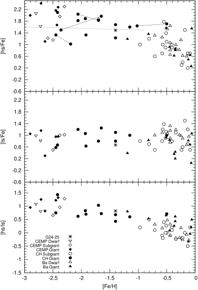
Figure 8: [$hs$/Fe], [$ls$/Fe] and [$hs/ls$] vs. [Fe/H] are shown in the three panels, from top to bottom, respectively. Dashed line separates stars belonging to the high and the low branches. Data have been collected from the following references: CEMP dwarfs - Lucatello et al. (2003), Sivarani et al. (2004); CEMP subgiants - Aoki et al. (2002b), Cohen et al. (2003), Tsangarides (2005), Cohen et al. (2006), Thompson et al. (2008); CEMP giants - Aoki et al. (2001, 2002b), Barbuy et al. (2005), Masseron et al. (2010); CH subgiants - Luck & Bond (1991), Pereira & Junqueira (2003), Pereira & Drake (2011); CH giants - Vanture (1992b, c), Kipper et al. (1996), Začs et al. (1998), Van Eck et al. (2001), Johnson & Bolte (2004), Goswami et al. (2006), Pereira & Drake (2009), Goswami & Aoki (2010), Masseron et al. (2010); Ba dwarfs - Allen & Barbuy (2006); Ba giants - Allen & Barbuy (2006), Pereira & Drake (2009).

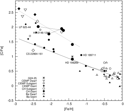
Figure 9: Comparison of [C/Fe] vs. [Fe/H] for chemically peculiar binary stars. The big and small sizes of one particular symbol represent stars with [Pb/Ba] $>$ 1 and [Pb/Ba] $<$ 1, respectively.

4 Conclusions

On the basis of high resolution and high $S/N$ spectra, the abundances of carbon and 12 neutron-capture elements, including Pb, are obtained for G 24-25. The C and $s$-process element abundances from the first, second, and third peaks show significant enhancements in this peculiar star with respect to the Sun and also with respect to a reference star G 16-20, which has similar atmospheric parameters as G 24-25. The abundance ratios [Pb/Fe] = 1.68 and [Pb/Ba] = 0.33 show that it is not a typical lead star (Van Eck et al. 2001), which are often found at low metallicity ([Fe/H] $<-2$) to have [Pb/Ba] $>1.0$. Owing to its binary signature, high radial velocity, and abundance pattern, we suggest that G 24-25 is a newly discovered CH subgiant with a clear detection of the Pb line at $\lambda 4057.8$.

Two simple AGB wind-accretion models have been adopted to predict the theoretical abundances of the $s$-process elements. The comparison of the observed abundances with the model predictions indicates that mass transfer via wind accretion across a binary system from its principal component, a low-mass AGB star, succeeds in reproducing the enhancements of the neutron-capture elements. When compared with other chemically peculiar binary stars in the literature, we have found that G 24-25 follows the general trend of [$s$/Fe], [$hs/ls$], and [C/Fe] versus [Fe/H] established for Ba stars, CH stars, and CEMP-$s$ stars implying that there is a similar origin for these objects.