Memory Hierarchy Sensitive Graph Layout

Abstract

Mining large graphs for information is becoming an increasingly important workload due to the plethora of graph structured data becoming available. An aspect of graph algorithms that has hitherto not received much interest is the effect of memory hierarchy on accesses. A typical system today has multiple levels in the memory hierarchy with differing units of locality; ranging across cache lines, TLB entries and DRAM pages. We postulate that it is possible to allocate graph structured data in main memory in a way as to improve the spatial locality of the data. Previous approaches to improving cache locality have focused only on a single unit of locality, either the cache line or virtual memory page. On the other hand cache oblivious algorithms can optimise layout for all levels of the memory hierarchy but unfortunately need to be specially designed for individual data structures. In this paper we explore hierarchical blocking as a technique for closing this gap. We require as input a specification of the units of locality in the memory hierarchy and lay out the input graph accordingly by copying its nodes using a hierarchy of breadth first searches. We start with a basic algorithm that is limited to trees and then extend it to arbitrary graphs. Our most efficient version requires only a constant amount of additional space. We have implemented versions of the algorithm in various environments: for C programs interfaced with macros, as an extension to the Boost object oriented graph library and finally as a modification to the traversal phase of the semispace garbage collector in the Jikes Java virtual machine. Our results show significant improvements in the access time to graphs of various structure.

1 Introduction

Modern computer systems usually consist of a complex path to memory. This is necessitated by the difference between the speed of computation and that of accessing memory, often referred to as the memory wall. While microprocessor performance has increased by 60% every year, memory systems have increased in performance by only 10% every year.

The typical solution employed by memory designers is to use faster smaller caches to cache data from larger but slower levels of memory. For example, a typical CPU cache would cache 64 byte lines from main memory while a Translation Lookaside Buffer (TLB) would cache mappings for 4KB chunks of virtual address space. A typical access to memory therefore has to negotiate many levels of hierarchy. Locality therefore has an important role to play for the in-memory processing of large datasets. If accesses are clustered (blocked) on the same 64 byte or 4KB chunk of memory (which we call units of spatial locality), it will lead to fewer transfers between levels in the memory hierarchy and consequently better performance.

Graphs form an important and frequently used abstraction for the processing of large data. This is more so today, with increasing interest in mining graph structured data: common examples being page-ranking that examines the hyperlinking between web-pages, community detection in social networks, navigational queries on road-network data or simulating the spread of epidemics (viruses) over human (computer) networks. Thus far, little attention has been paid to mitigating the impact of the memory hierarchy on processing large graphs. This paper makes the case that sensitivity to the memory hierarchy can make a big difference to the costs of processing large graphs.

Existing research along the same lines can be divided into two categories. The first category optimises object layout and connectivity taking into account only one level of the memory hierarchy. These algorithms however are suitable for use at runtime on arbitrary graphs. The second category are cache-oblivious algorithms that can optimise data structure layouts without knowing the precise hierarchy in use on the machine. Unfortunately cache-oblivious algorithms have been designed only for specific data structures and the techniques cannot be applied to graphs in general.

This paper proposes a Hierarchical Blocking Algorithm (HBA) as a solution. The HBA proposed in this paper takes arbitrary graphs as input and produces a layout that is sensitive to all levels of the memory hierarchy, information about which is supplied to the algorithm. We show that not only does this make a large difference to the processing of graphs, it also performs comparably to a cache oblivious layout. The HBA therefore, closes the gap between cache oblivious and cache sensitive (but limited to a single level) algorithms, an important contribution of this paper.

The rest of this paper is organised as follows. We begin with some intuition about HBA and describe how it is motivated by cache oblivious algorithms in Section 2. We then describe a basic version of HBA applicable only to trees in Sections 3, 4 and 5. We then provide extensions that make it applicable to arbitrary graphs in Section 6 and extensions for space efficiency in Section 7. We then describe implementation in three different environments (custom graph processing in C, Boost C++ graph libraries and the semispace garbage collector in the Jikes Java Virtual Machine) in Section 8. We then evaluate HBA and show that it delivers significant speedups in all these environments (from 10% to as much as 21X). We then discuss related work and possible future extensions to HBA, before concluding.

2 Motivation and Intuition

The hierarchical blocking algorithm we have developed draws strong inspiration from the van Emde Boas (VEB) layout. The VEB tree, originally proposed in a paper outlining a design for a priority queue veb is an arrangement that makes a tree data-structure cache oblivious i.e. likely to provide good performance regardless of the cache hierarchy or units of spatial locality in operation. The van Emde Boas(VEB) layout had provided some of the initial motivation for this work.

Figure 1 details the intuition behind the VEB layout. The VEB layout is a layout of a tree that is done by repeatedly splitting it at the middle and recursively laying out all the component subtrees in contiguous units of memory. In the figure, the tree of depth $D$ is split into a subtree (rooted at the original tree) of depth $\frac{D}{2}$ and this is recursively laid out first. Next, the remaining subtrees, $O(2^{\frac{D}{2}})$ in number, are laid out recursively. The VEB layout is complex to setup and maintain for trees and difficult to apply to graphs in general. The first step in applying it to a graph is to traverse the graph and prepare a sub-graph in the form of a tree that covers it. This spanning tree could then be laid out in a VEB layout. The key difficulty however is determining where to cut the tree since a-priori knowing the diameter of a graph and its splits at runtime is a difficult business. Further, the VEB layout does not consider heterogeneous graphs where the objects representing graph vertices may have different sizes, rendering it impractical to apply.

Our approach instead is to make the problem somewhat easier by assuming that the memory hierarchy (of caches) is known at runtime as an input to the algorithm. This can be used during the traversal to determine the spanning subtree in conjunction with information about the size of in-memory representations of graph vertices to determine the right split-point.

Figure 1: van Emde Boas Layout

Figure 2: Hierarchical Blocking Layout

Figure 2 shows graphically how this might be done. Assume an algorithm $P_{i}$ that aims to copy a tree while traversing it, into blocks that fit into the cache at level $i$. Using breadth first search, it can discover the entire subtree that fits into a block at level $i$. It can then call breadth first searches for individual subtrees that are rooted at the leaves of this subtree (not shown in the Figure). For the subtree it has identified, it can recursively call $P_{i-1}$: an algorithm that can lay out a given tree into blocks that fit into the cache at level $i-1$. This is shown in the Figure and corresponds (roughly) to the recursive layout achieved by VEB. The key difference is that we know where to cut the spanning tree based on runtime information about the memory hierarchy rather than simply using half the diameter of the graph.

Having provided intuition behind our Hierarchical Blocking Algorithm (HBA), we now proceed to discuss it in more detail below.

3 Hierarchical Blocking for Trees

In this section we develop a hierarchical blocking algorithm applicable to trees. A tree is a graph (either directed or undirected) where every vertex has a unique parent and is itself connected to a number of children. We express the algorithm in terms of repeated breadth-first searches cormen each of which is bounded to produce roots for new searches.

We begin by introducing some basic notation that we use in this section. We denote the application of an Algorithm $A$ to a graph vertex $x$ as $A(x)$, which produces as output a list of vertices. We denote application of an algorithm $A$ to a list of vertices $L$ by $A(L)$, which is done by applying it to each individual vertex and concatenating the outputs in order. We denote the repeated application of an algorithm (using the output of one as the input of the next) as $A^{k}$, which means that we apply algorithm $A$ $k$ times.

An important concept for hierarchical blocking is the space occupied by representations of a vertex. For a vertex $v$ we assume a way to measure the space occupied by the vertex, which we represent as $|v|$. This naturally extends to applying an algorithm $A$ on input $I$ as $|A(I)|$, which is just the sum of the spaces occupied by every vertex that is processed to produce the output.

The core algorithm is bounded breadth first search, which we abbreviate as $\text{BFS}_{d}$ that takes as input one vertex and produces a list of vertices that are at distance $d$ from the start vertex. We measure distance as the number of edges traversed. We also delegate to $\text{BFS}_{d}$ the job of copying traversed vertices into a spatially contiguous unit of memory.

We consider here a memory hierarchy of $n$ levels with monotonically increasing units of spatial locality: $s_{i}$ for level $i$, with $s_{i}<s_{i+1}$. We now define a blocking algorithm that takes as input a list of vertices and memory hierarchy levels, and recursively calls itself with decreasing levels. We denote the algorithm for level $i$ as $P_{i}$ taking as input a single vertex $o$. As indicated above, using $P_{i}$ on a list of vertices naturally follows from the definitions given below.

• $P_{1}(o)$ = $\text{BFS}_{d}(o)$ where we choose depth $d$ such that :

  • If $|\text{BFS}_{0}(o)|>s_{1}$ then $d=0$

  • Else choose $d$ such that $|\text{BFS}_{d-1}(o)|<s_{1}$ and $\text{BFS}_{d}(o)\geq s_{1}$

• $P_{i}(o):=P_{i-1}^{k}(o)$ where we choose $k$ such that:

  • If $|P_{i-1}(o)|>s_{i}$ then set $k=1$

  • Else choose $k$ such $|P_{i-1}^{k-1}(o)|<s_{i}$ and $|P_{i-1}^{k}(o)|\geq s_{i}$

At the start we are given the root of the tree: $r$. For hierarchical blocking of the tree, we repeatedly apply $P_{n}$ starting from $r$ until we have copied all the vertices (the output list is empty). The formalism given above produces exactly the layouts that we have provided an intuition for in the previous section. A crucial point to note here is that we allow the copying to overshoot the set limit by an amount bounded by one application of the algorithm at the next underlying level.

4 Analysis

A traversal of the tree needs to transfer blocks of size $s_{i}$ from the $i^{\text{th}}$ level in the memory hierarchy. We now provide an upper bound on the number of such blocks transferred. We make the observation that any application of $P_{n}$ can be ultimately expressed as repeated applications of $P_{i}$ for any $i<n$. Consider a traversal of the copied tree generated by $P_{i}(x)$ for an arbitrary vertex $x$ in the input graph. We consider a traversal that starts from the copy of $x$ produced by $P_{i}(x)$ and terminates at some leaf in the copied subtree produced by $P_{i}(x)$.

For any memory hierarchy level $j$ this traversal leads to the transfer of some number of blocks of size $s_{j}$. Let an upper bound on the number of memory blocks at level $j$ accessed due to this traversal be $B_{i}^{j}$, regardless of the start vertex.

Theorem 1.

$B_{i+1}^{i+1}=2+B_{i}^{i+1}$

Proof.  For any $x$: $P_{i+1}(x)$ is defined as $P_{i}^{d}(x)$ with $|P_{i}^{d-1}(x)|\leq s_{i+1}$. Now traversing a block of memory of size $s_{i+1}$ can incur accesses to at worst 2 blocks at level $i+1$ (if the block start is not aligned).

The remaining part of the traversal is to a subtree produced by $P_{i}(y)$ for some leaf $y$ of the previous traversal incurring at most $B_{i}^{i+1}$ block transfers. Hence we have: $B_{i+1}^{i+1}=2+B_{i}^{i+1}$ ∎

Under the common conditions where each level in the memory hierarchy is sufficiently smaller than the next level and $B_{1}^{1}$ fits within $s_{2}$ we can deduce a simple constant upper bound on $B_{i}^{i}$ for any $i$.

Theorem 2.

If $\;\;\;\forall j\;\;\;B_{1}^{1}<s_{2}\;\;\;\text{and}\;\;\;4s_{j}\leq s_{j+1}$ then $B_{i}^{i}\leq 4$

Proof.  The theorem is true at $i=1$ due to the conditions of the theorem where $B_{1}^{1}<s_{2}$ and $s_{2}$ is at most 4 blocks of $s_{1}$. We now give an inductive proof. Let the theorem be true till $i=k$. We have $B_{k+1}^{k+1}=2+B_{k}^{k+1}$. From the induction hypothesis $B_{k}^{k}\leq 4$. Four blocks at level $k$ is at most one misaligned block at level $k+1$ (due to the bounds on sizes at each level) which is at most two aligned blocks at level $k+1$. Hence $B_{k+1}^{k+1}\leq(2+2)=4$ ∎

In the context of the whole tree a traversal from root to leaf in the copied tree incurs repeated costs of $B_{n}^{i}$ at memory hierarchy level $i$. If we assume that $P_{i}(x)$ covers subtrees of depths at least $d_{i}$ then the number of block accesses at memory hierarchy level $i$ for a traversal of depth $D$ is bounded by $4\frac{D+1}{d_{i}+1}$. For a pseudorandom allocation of vertices to memory, one would normally expect every access to cause a transfer, leading to $D+1$ transfers. The hierarchical blocking algorithm is therefore able to guarantee reduced transfers when $d_{i}>3$.

Note that this is a pessimistic upper bound. For example, at the lowest level (usually cache lines) any organisation that packs subtrees of depth one into a cacheline leads to better performance with one cacheline serving two access requests instead of one.

5 Iterative Version

We now present an iterative version of the hierarchical blocking algorithm (HBA). In addition to being easier to understand, implement and analyse; it forms the basis for extension to handle arbitrary graphs. The HBTreeIterative algorithm listed in Procedure 1 is a direct translation of the recursive algorithm described in the previous section. It takes as input a root vertex and a description of a memory hierarchy and performs runtime hierarchical blocking of the tree rooted at the supplied vertex. Starting from this section, we introduce the term ’node’, that we use as an abstraction for the memory occupied by a graph vertex (and any associated edge data structure, such as an edge list).

Procedure 1 HBTreeIterative

0:  root: root to block from

0:  n: levels of hierarchy

0:  s[1..n]: block sizes (monotonically increasing)

0:  s[n+1] = INFINITY

1:  Initialise to empty: Dequeue roots[1..n+1]

2:  Initialise to empty: Dequeue leaves[1..n+1]

3:  Initialise to zero: space[1..n+1]

4:  roots[n+1].push_back(root)

5:  level := n + 1

6:  loop

7:     if roots[level].is_empty() then

8:        ////////Refill

9:        roots[level] := leaves[level]

10:        leaves[level] := empty

11:        if space[level] $\geq$ s[level] then

12:           //////Promote

13:           leaves[level + 1].append(roots[level])

14:           roots[level] := empty

15:           space[level + 1] := space[level + 1] + space[level]

16:           level := level + 1

17:           continue loop

18:     if roots[level].is_empty() then

19:        //////Promote

20:        if level = (n + 1) then

21:           TERMINATE

22:        else

23:           space[level + 1] := space[level + 1] + space[level]

24:           level := level + 1

25:     else

26:        node := roots[level].pop_front()

27:        if level $>$ 1 then

28:           //////Push work down

29:           roots[level - 1].push_back(node)

30:           space[level - 1] := 0

31:           level := level - 1

32:        else

33:           /////Do some copying work

34:           if UnconditionalCopyNode(node) then

35:              space[1] := space[1] + sizeof(node)

36:              leaves[1].append(children(node))

Procedure 2 UnconditionalCopyNode

0:  node: node to copy

1:  Copy node to tospace

2:  tospace := tospace + sizeof(node)

3:  Update parent of node in tospace to point to copy

4:  return  true

The core data structures used in the algorithm are lists of roots and leaves for each level of the hierarchy. In addition the space array maintains the amount of space used at each level. Lines 34–36 of the algorithm implement $\text{BFS}_{d}$. This is done by taking the root node for the BFS, copying it (through the call to UnconditionalCopyNode and updating the space used. The children produced during this BFS step are added to leaves[1]. If the amount of space used is less than the unit of spatial locality for hierarchy level 1, all the leaves of the BFS are moved to roots[1] and a BFS step is subsequently performed for each of them to uncover their children. Thus, only when the total space consumed at this lowest level is equal to, or exceeds the unit of spatial locality at the lowest level, is the level variable bumped and all the produced leaves of the BFS moved to level 2. It is easy to see that this replicates the operation of $\text{BFS}_{d}$ described in the previous section and discovers $d$ dynamically.

For any $\text{level}=i>1$, the remaining steps of HBTreeIterative implement $P_{i}$. Recall that the input to $P_{i}$ is a list of nodes, this is held in roots[i]. Lines 11-17 check whether repeated applications of $P_{i-1}$ have exhausted the unit of spatial locality given by $s[i]$. If so, the output leaves are passed on to level $i+1$. Else, we repeatedly call $P_{i-1}$ on the head of the $roots[i]$ list. Finally, the level n + 1 is simply a placeholder for the output of $P_{n}$. For convenience, it is assumed to have an infinite amount of spatial locality, i.e. it covers the whole memory.

Copying services are provided by UnconditionalCopyNode that copies nodes into a region of memory whose top is held in the tospace variable. We assume that this region of memory is infinite. A practical implementation of UnconditionalCopyNode could simply call a standard heap allocation function (such as malloc) to allocate memory to copy into, although this inserts metadata before the copied object that can reduce locality (as we discuss later).

Figure 3: Small Example Tree

In order to better understand the operation of
HBTreeIterative, consider the graph of Figure 3. If the input to HBTreeIterative is the node a then the first thing the algorithm does is to add a to roots[n+1]. The node a then bubbles down to roots[1] through repeated iterations of the loop. It is then passed to
UnconditionalCopyNode at line 34. Next, line 36 adds its children, nodes b and c to leaves[1]. Since roots[1] is now empty, both b and c are copied into roots[1] at line 9. Assume for this example that at least one node fits into s[1] and so b and c are processed in turn resulting in roots[1] containing d, e, f, and g. If now the algorithm finds space[1] > s[1] then it promotes these four nodes to level 2 and then calls $P_{2}$ on them (unless s[2] is also exhausted). This finally results in a consecutive layout in memory of nodes a, b and c, followed by (partial) subtrees rooted at d, e, f and g produced by $P_{2}$.

5.1 Complexity

Given a tree with $N$ nodes and $E$ edges, the HBTreeIterative algorithm performs a graph traversal on it. It visits every edge exactly once (in line 36). For any node, after discovery, the node is added to every one of the root and leaf lists at most once. Hence, given $L$ levels in the memory hierarchy the algorithm has a worst-case complexity of $O(LN+E)$. In a tree the number of edges is one less than the number of nodes and hence the complexity is $O(LN)$. Note that in practice with settings such as $s[1]=64$ for and $s[2]=1024$ (used in this paper) most nodes are only added to lists at levels 1 and 2 before being processed and never make it to higher levels. Practically, this keeps the overhead of the algorithm (and its variants) close to $O(N+E)$ or $O(N)$ for trees.

5.2 Limitations

A key limitation of HBTreeIterative is that it applies only to trees. There are two reasons why it cannot be used on arbitrary graphs. The first is that UnconditionalCopyNode expects that it is passed any node exactly once. This is easily violated in the case of multiple parents (as in directed acyclic graphs) or graphs with cycles. A related problem arises because more than one pointer may exist to a node and hence UnconditionalCopyNode should be able to update parent pointers even if the node has already been copied. In the next section we describe extensions to HBTreeIterative that allow it to be used on arbitrary graphs.

6 Extension to Arbitrary Graphs

Extending HBTreeIterative to arbitrary graphs first requires lowering our level of abstraction somewhat. Along these lines, we introduce the notion of a slot. A slot is simply a pointer to a node. Any given arbitrary graph is therefore ’rooted’ at multiple slots. Readers familiar with garbage collectors in Java will notice that we have borrowed these two terms from there gc_book .

Processing an arbitrary graph requires processing each root slot in turn. This is done by calling InitiateCopy in Procedure 3. For every given root slot, it calls HBTreeIterative thereby processing individual components of the graph. Note that we do not require graphs with different roots to be unreachable from each other.

Procedure 3 InitiateCopy

0:  roots: queue of slots to start copying

1:  while not roots.is_empty() do

2:     slot := roots.pop_front()

3:     HBTreeIterative(*slot, levels, Sizes[1..levels])

The only change we make to HBTreeIterative is to call ConditionalCopyNode at line 34 instead of
UnconditionalCopyNode. Procedure 4 describes the former. The major change is the introduction of the Forward table that has an entry for each possible node, indicating whether that node has been forwarded. If not already forwarded, it forwards (determines the position in tospace) the node and returns an appropriate indication. HBTreeIterative then uses the returned indication to ensure that every node is considered at most once thereby solving the problem of multiple parents and cycles encountered in arbitrary graphs.

Procedure 4 ConditionalCopyNode

0:  node: node to copy

1:  if Forward[node] = UNFORWARDED then

2:     Forward[node] := tospace

3:     tospace := tospace + sizeof(node)

4:     return  true

5:  else

6:     return  FALSE

Procedure 5 CompleteCopy

0:  roots: list of pointers to start copying

1:  while not roots.is_empty() do

2:     slot := roots.pop_front()

3:     if not Copied[*slot] then

4:        Copied[*slot] = true

5:        Copy *slot to Forward[*slot]

6:     *slot := Forward[*slot]

7:     for all child_slot pointers in *slot do

8:        roots.push_back(child_slot)

Since ConditionalCopyNode no longer updates pointers or copies nodes, we introduce a post-processing phase called CompleteCopy. This is shown in Procedure 5 and is called after InitiateCopy has completed. It traverses the graph starting at the roots again and maintains a Copied map to avoid copying a node more than once. It also updates all the slots to point to the copies in tospace.

6.1 Complexity

We now consider the complexity of InitiateCopy,
HBTreeIterative and CompleteCopy taken together. Slots now explicitly represent edges in the graph. Every slot (edge) is still considered at most once (or twice if it is a root slot), this includes lookups in the extra maps. Any given node is also processed at most once at copying and enters (and leaves) every one of the $L$ lists at most once. Hence the asymptotic complexity of the algorithm remains at $O(LN+E)$.

6.2 Limitations

The extensions to deal with arbitrary graphs suffer from two key problems. The first problem naturally is the need to have two passes through the graph. The second problem is the space cost of maintaining the extra maps. A related problem that we have not thus far considered is the cost of maintaining the root and leaf dequeues. Even maintained as linked lists (as we do) they require one next pointer per node. Note that the space overheads are bounded by $O(N)$ and do not depend on the number of edges. Nevertheless, it is desirable to try to eliminate them.

In spite of these limitations, we use an actual implementation of the generalised HBA described in this section in the evaluation. For applications where offline Reorganisation of large graphs is acceptable it is simple to implement and effective.

7 Single-Pass and Possibly Metadata-Less Blocking

We now introduce the final and most sophisticated HBA. Before introducing the algorithm, we make some observations about the operation of HBTreeIterative in the case of general graphs. For any node that is copied, all its unvisited children are added as a group to leaves[1]. This group of nodes continues unbroken through various lists until it enters a roots list. After that they are dequeued in order to be bubbled down and copied. Note that once a node is picked off a roots list at line 26 of HBTreeIterative it is copied immediately.

The key idea we take away from this observation is that it is possible to represent this group of nodes by its parent. Once the group (parent) enters a roots list, instead of popping the parent, we pop slots in the parent one by one and bubble them down in turn to be processed. Processing the slot involves both conditionally copying the target and updating the slot to point to the new version of the node. We now introduce HBGraphOnePass that incorporates these ideas. Unlike the version for trees, it takes as input the root slot to start processing from (and not the root node pointed to by that slot). It still depends on (a slightly modified for interface reasons) InitiateCopy to iterate through roots but eliminates CompleteCopy.

Procedure 6 HBGraphOnePass

0:  root_slot: root slot to block from

0:  n: levels of hierarchy

0:  s[1..n]: block sizes (monotonically increasing)

0:  s[n+1] = INFINITY

1:  Initialise to empty: Dequeue roots[1..n+1]

2:  Initialise to empty: Dequeue leaves[1..n+1]

3:  Initialise to zero: space[1..n+1]

4:  level := 1

5:  /////Conditionally copy root slot

6:  old_node := *root_slot

7:  if CopySlot(root_slot) then

8:     space[1] := space[1] + sizeof(*root_slot)

9:     leaves[1].append(old_node)

10:  loop

11:     if roots[level].is_empty() then

12:        ////////Refill

13:        roots[level] := leaves[level]

14:        leaves[level] := empty

15:        if space[level] $\geq$ s[level] then

16:           //////Promote

17:           leaves[level + 1].append(roots[level])

18:           roots[level] := empty

19:           space[level + 1] := space[level + 1] + space[level]

20:           level := level + 1

21:           continue loop

22:     if roots[level].is_empty() then

23:        //////Promote

24:        if level = (n + 1) then

25:           TERMINATE

26:        else

27:           space[level + 1] := space[level + 1] + space[level]

28:           level := level + 1

29:     else

30:        slot := roots[level].pop_front_slot()

31:        for all i $>$ 1 and i $<$ level do

32:           //////Init level

33:           space[i] := 0

34:        level := 1

35:        /////Do some copying work

36:        old_node := *slot

37:        if CopySlot(slot) then

38:           space[1] := space[1] + sizeof(*slot)

39:           leaves[1].append(old_node)

Procedure 7 CopySlot

0:  slot: slot to copy

1:  copied := false

2:  if Forward[*slot] = UNFORWARDED then

3:     Forward[*slot] := tospace

4:     tospace := tospace + sizeof(*slot)

5:     copy *slot to Forward[*slot]

6:     copied := true

7:  *slot := Forward[*slot]

8:  return  copied

HBGraphOnePass also uses a slightly different helper routine CopySlot to complete copying of nodes. It directly updates the slot with the copy of the node. Assuming that copying was required the node is then explored for children. Note that in line 39 of HBGraphOnePass we append the old node to the leaves[1] list. This node is bubbled up and ultimately moves to a roots list. In line 30, instead of popping the node, we pop its children one by one. This can be implemented by maintaining constant sized state about which child has been popped. Note that we hoist a copy of part of the processing for the root_slot to lines 6–9.

Other than these changes HBGraphOnePass operates similarly to HBTreeIterative. To illustrate this, consider again the example graph in Figure 3. The algorithm is passed the slot pointing to node a. It then copies node a and adds a itself to leaves[1]. Assuming s[1] is not exhausted a then moves to roots[1]. Slots containing children of a are then popped off by the call to pop_front_slot and this b and c are copied next. Tracing the operation further, it should be evident that HBGraphOnePass produces the same layout in memory as HBTreeIterative for the example.

7.1 Complexity

The complexity analysis for HBGraphOnePass is substantially the same as in the previous section. Every slot is considered at most once from lines 30–39 of HBGraphOnePass (other than being passed in as a root slot). Nodes traverse every list at most once. Thus HBGraphOnePass also has an asymptotic complexity of $O(LN+E)$.

7.2 Eliminating Metadata

A simple observation also serves to eliminate the need for $O(N)$ extra metadata. All nodes in a graph would have at least one pointer worth of space (unless the graph is using a particularly compressed format). Further if the graph is to represent any form of branching it would have space for at least two pointers in its node representation.

We use the first available pointer to store a pointer to the forwarded copy. This eliminates to need for the Forward table since slots that need copying point to old objects that can be looked up to determine the forward pointer. In our implementations, we set the last bit to distinguish the forward pointer from the same field in objects that have not yet been copied (since they would point to objects aligned at 4 byte boundaries in our implementation). Further, we can use the other available pointer for manipulation of the lists representing the dequeues. This eliminates the need for any external metadata, removing the need for $O(N)$ extra space.

Note that this elimination is made possibly by the organisation of HBGraphOnePass that uses parent nodes to represent groups of children. In the absence of this observation, we would have been forced to use dequeues of slots in order to eliminate the extra pass thus rendering impossible elimination of extra metadata for the dequeues. Further, this metadata-less one pass HBGraphOnePass algorithm is a significant advancement over previous work. Cheney cheney had shown that it was possible to use a breadth-first traversal over objects in the heap without the need for any extra metadata. Although Wilson wilson had developed hierarchical BFS for a single level, it required one pointer per page of memory. HBGraphOnePass subsumes Wilson’s algorithm as a special case of a single-level memory hierarchy and also admits implementation without the need for extra metadata, similar to Cheney’s copying algorithm.

Of course, the technique described in this subsection is optional. For example one could also allocate the extra $O(N)$ metadata directly in objects, such as we have done for integration with the Jikes Java Virtual Machine jikes garbage collector in one of our implementations. There, the forwarding pointer already existed in the object header and we found it simplest to just add another field for manipulation in the dequeue lists.

8 Implementations

In this section we describe three different environments into which we have integrated versions of our HBA. This section focuses on graph representation and concrete interfaces for HBA. Another important focus area for this section is memory allocation. Allocating target memory for copied nodes can broadly follow one of two strategies. One is to use the system provided memory manager that is already in use. This has the advantage of integrating cleanly with existing code that uses graphs since there is no need to write an additional memory manager and allocated nodes can be freed by the rest of the application. A disadvantage to this approach is that system memory managers (such as malloc) introduce additional metadata at the head of each object. This should be taken into account when calculating object sizes in the HBA and additionally reduces the effectiveness of blocking in improving spatial locality. Also, memory managers such as malloc often use discontiguous pools for objects of different sizes. This introduces further fragmentation if graph nodes are differently sized, which is often the case for variable sized edge lists attached to the nodes. The other option is to use a memory manager with external metadata to manage to space copied to, which can introduce the complexity of using multiple memory managers.

We have implemented HBA in three environments for evaluation: custom graph implementations written in C, as an add-on to the Boost Graph Library in C++ and finally as a modification to the traversal phase of the semispace copying collector in the Jikes Java Virtual Machine. We now discuss these implementations individually.

8.1 Boost C++ Graph Library

The Boost C++ Graph Library (BGL) boost is a library for in-memory manipulation of graphs. It makes extensive use of C++ generics (making extensive use of templates) to provide a customisable interface for storing graph structured data. We wrote an extension to the library that takes as input a graph stored in the adjacency list representation and produces a new graph after hierarchical blocking. The adjacency list representation stores a list of vertices in an iterable container, that allows one to iterate over every vertex in a graph and then apply a suitable function. For each vertex the list of edges originating at (for directed graphs) or connected to (for undirected graphs) is maintained in another iterable container attached to the vertex. Although our implementation is generic, we experimented with C++ STL vectors as the container for both the types of components.

Our HBA addition to Boost uses the simpler version of the algorithm described in Section 6. It makes use of two external $O(N)$ sized vectors and assumes a canonical mapping from the set of vertices to non-negative integers: $f:V\rightarrow\{1\;\;..\;\;|V|\}$. This is already provided by Boost and we use this integer to index into the $O(N)$ sized vectors. The first vector is used to maintain a “next” pointer ($f(\text{next})$ rather than next). The second vector (we call it the RemapVector) assigns, for each given node in the input graph a number indicating its position in the copied graph i.e if RemapVector(j) = RemapVector(i) + 1 then node j should be copied right after node i in the output graph. It is easy to see how the remap vector is set up by calls to ConditionalCopyNode. We use the produced remap vector in CompleteCopy to actually produce the output graph.

We use the memory allocator provided by Boost thereby incurring the overheads described above. We have assumed for object size calculation that each edge occupies an area equal to three pointers (for source, destination and edge-weight information) and two pointers worth of memory management metadata. Since the vertices are already laid out in a vector, we multiply the number of outgoing edges by the space occupied by five contiguous pointers to determine the object size for the HBA algorithm.

Our decision to use the simpler algorithm for integration into Boost was guided in part by the observation that others have deemed the overheads of storing all the vertices of a graph in memory acceptable semiem .

8.2 Custom Graph Implementations in C

The Boost graph library introduces a number of overheads internal to the objects used to represent graph vertices and edges, in part due to the need to be generic and object-oriented. In order to explore the benefits that HBA can bring to graphs constructed out of carefully designed minimal objects we also wrote a custom implementation of binary search trees and undirected graphs for evaluation. For the C implementations, we allocated a large chunk of memory to copy the nodes into, this is done by maintaining the size of the graph as it is loaded and calculating the total space required for the copy, in advance. This eliminates all overhead due to memory manager metadata. It is easy to write a memory manager that makes use of external metadata vee to manage this space, although we have not done so for this implementation.

8.2.1 Binary Search Trees

We use the fairly minimalist representation of binary search tree nodes shown below:

/* Basic bst node */
typedef struct node_st {
  unsigned long k; struct node_st *l, *r;
#ifndef NO_REORG_PTR
  struct node_st **reorg_next;
#endif
}node_t;

We have explored both HBTreeIterative (that makes use of the reorg_next pointer) as well as HBGraphOnePass that eliminates that pointer.

8.2.2 Undirected Graphs

We have also written representations for undirected graphs in C. These make use of the data structures described below:

typedef struct node_st {
  int id;  struct node_st* neighbours[0];
} node_t;

node_t **node_vector;
int *neighbour_cnts;
int node_cnt;

The graph node structure contains an integer identifier and an array of pointers to its neighbours. Since this is an undirected graph, two neighbouring nodes point to each other through their neighbours arrays. In addition, we have a list of vertices (node_vector), a list of neighbour counts (neighbour_cnts) and finally the count of the total number of nodes in the graph (node_cnt). Maintaining the size of the neighbours array outside the data structure improves cache-line utilisation. Note that as with the Boost implementation, we have an enumeration of vertices as integers that allows indexing appropriate arrays. A point that might not be evident is that HBA also results in better utilisation of linear arrays such as neighbour_cnts. This is because adjacent nodes are more likely to be placed close to each other in those arrays. This was key to our decision to move the neighbour count out of the containing node_t object.

Finally, we also wrote an extension to our implementation of undirected graphs to illustrate a beneficial and powerful application of the HBA algorithm. We allow the writing out of the entire graph after HBA to disk. The nodes are written out in the order that they are produced by HBA. Therefore, reloading the nodes results in an in-memory representation of the graph that is already blocked. Although we show in our evaluation that the overheads of HBA are tolerable enough to apply at runtime, this feature serves to illustrate that offline HBA of in-memory graphs and storing the results in a persistent manner is very much possible and eliminates the overheads of HBA when processing static graphs.

8.3 Jikes RVM

We have also implemented HBA as an extension to the traversal phase of a semispace copying collector in the Jikes Java Virtual Machine. We have done this to illustrate the ability of HBA to operate in dynamic environments with varying graphs. The fundamental idea of the semispace copying collector is to divide the heap into two ’spaces’. At any instance of time only one space is ’active’, and is used to allocate objects. When a garbage collection is triggered, all mutator threads (that can change the connectivity or contents of objects on the heap) are stopped. A collector thread then runs a traversal phase that finds all reachable objects on the heap using a depth-first search in the baseline implementation and copies them (on discovery) to the other ’inactive’ space. After completion of this traversal, the ’inactive’ and ’active’ spaces switch roles until the next garbage collection cycle.

We have modified the traversal phase to use HBA in order to copy objects with appropriate clustering. We use the single pass HBGraphOnePass algorithm. Since the object-header used in the Jikes RVM had already allocated a pointer to hold miscellaneous information, we used this pointer to hold forwarding information. We added another pointer size field to hold next pointer information for maintaining the dequeues. We use this slightly bloated object representation as the baseline (without HBA) as we felt that this fairly reflected the fact that we could have eliminated this overhead with extra work. Our implementation in the Jikes RVM is at a prototype level only, in part to avoid the complexity of refactoring the garbage collection classes to implement an optimised version. For example, it is difficult to interrupt the scanning of objects on the heap to determine slots. Hence we have a suboptimal implementation of pop_front_slot that simply uses an array of 32 slots to hold the results of a complete scan. Any overflows from this array are treated as new roots by the HBA implementation. Nevertheless, we found the implementation adequate to demonstrate the feasibility of integrating HBA into the garbage collector of a managed environment, thereby showing that is can be used in such environments and on changing graphs.

9 Performance Evaluation

We evaluate HBA on an system equipped with an Intel i5-2400S CPU and 16 GB of RAM. For uniformity (the JikesRVM is 32-bit only) we use 32 bit code and thus are limited to using under 4GB of main memory. We know a-priori that the system has the following caches in its memory hierarchy (with corresponding settings for the HBA):

1. Various caches (L1 data, L2 and L3) with a 64 byte line size. We set s[1] = 64.

2. Open-page mode DRAM that provides lower latencies for consecutive accesses to the same 1024 byte page. We set s[2] = 1024.

3. TLB caching page table translations for 4KB pages. A TLB miss incurs significant penalty for page table walks. We set s[3] = 4096.

4. TLB caching of super page translations. The OS (linux) clusters groups of pages into 2MB superpages to reduce consumption of page table and TLB entries. We set s[4] = 2097152.

It is unclear to us (as it would be to users of HBA in the field) about which level is most likely to impact performance for a particular graph and particular traversal algorithm. Hence we usually use full HBA with the settings above, indicated as HBA(all) in the evaluation. Occasionally we use HBA for only a subset of levels: such as the page level HBA(4k), this is essentially produces the layouts of Wilson’s hierarchical BFS wilson .

9.1 C, Binary Search Tree

We first consider the performance of a binary search tree written in C. The tree is setup to hold a contiguous integer keyspace and is then queried with random keys. We are interested in the average query time (measured over a minute of continuous queries) as the traversal is affected by the locality of the nodes. We investigate the following layouts of tree nodes in memory: 1. Psedorandom layout 2. BFS layout ((such as would be produced by Cheney et. al. cheney ) 3. DFS layout, some researchers have suggested that this might be a better way to layout nodes for locality than BFS stamos 4. VEB layout and finally 5. HBA layout using the algorithm in this paper.

The results are shown in Figure 4. As expected the pseudorandom layout performs the worst. BFS performs better than DFS. The best performance is provided by HBA, which performs almost comparably to VEB. At a tree depth of 25 ( 64 million nodes) using HBA reduces query time by approximately 54% while using BFS reduces query time by approximately 31%. A notable feature of the graph is the knee around the tree depth of 18. This is because beyond that depth the tree no longer fits in the 6MB last level cache leading to a sudden increase in query time.

Figure 4: Binary Search Tree Performance

Not every level of cache has an equal impact on performance. To illustrate this, we ran the same experiment restricting HBA to various subsets of the memory hierarchy. The results, shown in Figure 5 illustrate that the cache (64 byte units of spatial locality) and the VM page (4K unit of spatial locality) have the maximum impact on tree access.

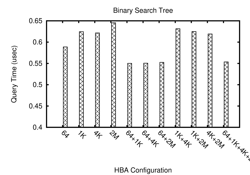
Figure 5: Varying HBA parameters

Finally, we verify that HBA is indeed improving cache access. We used cachegrind cachegrind to instrument the queries and simulate various levels of the memory hierarchy of the actual system. Table 1 shows the miss rates for various levels of the hierarchy. Although DFS and BFS both improve miss rates, HBA is most effective at reducing miss rates, explaining its better performance. It is interesting to note that HBA when run over all levels reduces miss rates for any level to that produced by running HBA to block only for that level. This is an important result, since it illustrates that HBA provides additive benefits for all the memory hierarchy levels it is aware of. Finally, we note that HBA is almost as effective at tackling miss rates as the cache-oblivious VEB layout.

	L1d line	DRAM page	VM page	VM superpage
Pseudorandom	0.42	0.53	0.44	0.42
BFS	0.36	0.43	0.26	0.07
DFS	0.33	0.23	0.19	0.11
VEB	0.24	0.15	0.05	0.02
64	0.25	0.19	0.10	0.03
1K	0.31	0.19	0.07	0.02
4K	0.32	0.25	0.07	0.02
2M	0.33	0.34	0.14	0.02
64+1K+4K+2M	0.25	0.17	0.06	0.02

Table 1: Cachegrind miss rates

Finally, we illustrate the effect of removing HBA related metadata from the tree node, using the HBGraphOnePass algorithm and reusing pointer fields from the old version of the object (as discussed in Section 7.2). The results shown in Figure 6 illustrate the improvements obtained due to the lower memory footprint of the tree nodes: approximately 14% lower than that with an extra pointer per tree node.

Figure 6: Binary Search Tree: Effect of removing HBA metadata

9.2 Arbitrary Graphs

Trees represent an ideal workload for HBA, since they correspond exactly to the spanning tree built during traversal. In this section, we consider more complex graphs with a large number of connections. We use a synthetic graph generator that is part of the SNAP suite snap . We consider various kinds of graphs that are of current interest to the research community involved in mining information from graph structured data:

1. Watts-Strogatz small world model watts (10 million nodes, 29 million edges): These graphs have logarithmically growing diameter and model small world networks, such as social networks with the informally well known “six degrees of separation”.

2. Barabasi-Albert model albert (10 million nodes, 39 million edges) also models real world phenomena but provides graphs where the out-degree of nodes follows a power law distribution. This is often the case, for example, with web pages that link to each other.

3. 2d mesh (9 million nodes, 17 million edges) models real world road networks. Answering real time navigational queries on such networks are often a component of many online services.

4. 4ary tree (10 million nodes, one less edge). To provide some perspective on binary trees considered thus far, we also measure performance on trees where each node has 4 children.

We use two different algorithms (in two different implementations). The first is a single source shortest path algorithm (using Dijkstra cormen ) that finds shortest paths from a given source to all nodes in the graph. We use a random assignment of wights to edges (a uniform random choice over a range of size the same as the number of vertices). We use an implementation of this algorithm in Boost (Section 8.1). We then turn the input graph into an undirected and unweighted version by adding a reverse edge for every given edge and performing a breadth-first search in our custom C environment (Section 8.2). The choice of algorithms and datasets is fairly similar to other approaches that evaluate the performance of graph processing solutions semiem .

For each algorithm, data set and environment we measure the speedup of the algorithm after HBA on the graph using both HBA(4k) as well as HBA(all) i.e. blocking for VM pages and for all levels of the hierarchy respectively. The results shown in Table 2 underscore the efficacy of HBA for arbitrary graphs. Large speedups (as high as 21X !) are obtained with HBA. Speedups are generally higher for our custom C environment due to the optimised (reduced) object footprints. Optimising for all levels of the memory hierarchy often provides better performance than just optimising for one level, underscoring the importance of a multi-level blocking algorithm. The results also illustrate an interesting example of destructive interference between levels. HBA(4k) performs slightly better than HBA(all) in the case of 2d meshes. Other than this example, we have found that in all cases HBA(all) performs at least as well as HBA(4k).

Graph	SSSP		BFS
	HBA(4K)	HBA(all)	HBA(4k)	HBA(all)
Watts_Strogatz	1.41	1.44	1.38	1.40
Albert_Barabasi	1.01	1.02	1.09	1.11
2d_mesh	2.38	2.35	3.85	3.80
4ary_tree	1.00	1.00	20.70	21.31

Table 2: Graph Processing Speedups

9.3 JikesRVM

Our final set of results are from the Jikes Java Virtual machine. We measured the performance of the same binary search tree considered in the C environment, when implemented in Java. We configured the JVM to use a 1GB heap for the experiments. We also configured it to perform a system-wide GC before starting the query phase of the test. The results, shown in Figure 7 indicated that the benefits seen with C are also replicated in the Java environment. HBA for all levels with a tree depth of 22 provides a 29% speedup over the baseline version, while HBA for only the VM page provides a 19% speedup over the baseline version. Note that JVM memory limitations meant we were unable to build trees of larger depth.

Figure 7: Binary Search Tree: JikesRVM Performance

In a runtime environment the overhead of collection is also an important factor. With this in mind, we measured the time for a semispace copy of the entire heap after the tree has been completely built. The results are shown in Figure 8. In the worst case, HBA adds an overhead of only 18%. Crucially the overhead of optimising for all levels is the worst case only 10% more than optimising for only the page level. The average overheads are much lower, well under 10%.

Figure 8: Binary Search Tree: Semispace collector overheads

Finally we also measure overheads and performance with the more general DaCapo benchmark suite dacapo . The results shown in Fig 9 indicate that the overhead of adding HBA to the garbage collector is under 15% in all cases and usually under 10%. In addition for two of the benchmarks (antlr and fop) we see improved performance due to more locality on the heap.

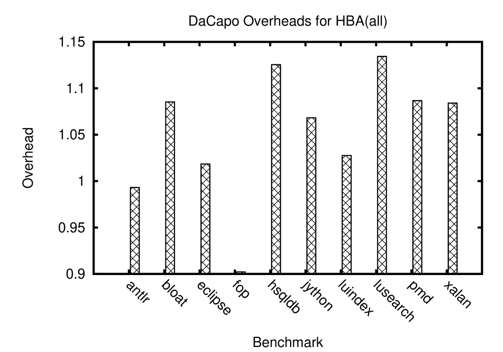
Figure 9: DaCapo Benchmarks: Semispace collector overheads

10 Related Work

There is a large body of existing research into improving the cache performance of in-memory data. Broadly the approaches can be divided into three classes.

The first class of techniques deal with prefetching objects ahead of use. An example of this is the approach of Luk et al. rds_prefetch , who place a prefetch pointer in linked list nodes to prefetch later nodes early enough to avoid cache miss penalties during traversals. Dynamic approaches are also possible such as that of Chilimbi et al. who profile a program to detect frequently occurring streams of accesses chilimbi_hot .

A second class of techniques is to statically modify the data structures themselves to make them more cache friendly. One way is to use knowledge of the cache hierarchy and transfer units to size data structure nodes, such as in B-trees  cormen . This can be extended to make the B-tree nodes cache friendly at various levels (similar to the objective of this work). Kim et al. fastbtree extend the basic idea of B-trees to be architecture sensitive at various levels using hierarchical blocking. Although their hierarchical blocking produces layouts similar to our reorganisation algorithm they have a static data structure redesign for B trees unlike our dynamic general purpouse algorithm. Another approach to data structure design is cache oblivious data structures. These are designed so as to improve spatial locality regardless of the level of memory hierarchy and block size being considered. The “van Emde Boas” layout veb forms the basis for many cache oblivious designs including those for cache oblivious B-trees streamingbtree .

A third class of techniques (including the one in this paper) are used at runtime. One approach is to control memory allocation. Chilimbi et al. chilimbi_cc_layout investigated the use of a specialised memory allocator that could be given a hint about where to place the allocated node. Another approach is to use the data structure traversal done by garbage collectors to copy objects into new cache friendly locations copying . Mark Adcock in his PhD thesis adcock_phd considered a range of runtime data movement techniques including those triggered by pointer updates. However none of these techniques consider the effect of multiple units of locality in the memory hierarchy and in that sense this work is orthogonal to all of them. It is possible to take the algorithm in this paper and use it to improve on all of these locality maximisation techniques, which are usually restricted to plain breadth-first search to discover nodes.

11 Future Work

The current implementation of HBA ignores the last level in a usual memory memory hierarchy: persistent storage. It is extremely easy to add a 512 byte sector size to HBA to also optimise layouts for transfer from disk. Although we have not investigated this aspect yet, we believe HBA can also significantly improve access to the last (persistent) level in typical memory hierarchies.

12 Conclusion

We have presented a hierarchical blocking algorithm (HBA) that takes as input an arbitrary graph and a description of a memory hierarchy and lays out graph nodes to be sensitive to and provide better performance for that hierarchy. We have investigated implementations of HBA in various settings and shown that it provides non-trivial benefits in all of them; making the case the graph layout and memory hierarchy sensitivity are important factors in the performance of graph algorithms.

References

- [1] http://jikesrvm.org/.
- [2] http://www.boost.org/doc/libs/graph/.
- [3] http://valgrind.org/info/tools.html#cachegrind.
- [4] http://snap.stanford.edu/snap/.
- [5] Mark Adcock. Improving cache performance by runtime data movement. Technical Report UCAM-CL-TR-757, University of Cambridge, Computer Laboratory, July 2009.
- [6] Reka Zsuzsanna Albert. Statistical mechanics of complex networks. PhD thesis, Notre Dame, IN, USA, 2001. AAI3000268.
- [7] Michael A. Bender, Martin Farach-Colton, Jeremy T. Fineman, Yonatan Fogel, Bradley Kuszmaul, and Jelani Nelson. Cache-oblivious streaming b-trees. In Proceedings of the Nineteenth ACM Symposium on Parallelism in Algorithms and Architectures, pages 81–92, 2007.
- [8] S. M. Blackburn, R. Garner, C. Hoffman, A. M. Khan, K. S. McKinley, R. Bentzur, A. Diwan, D. Feinberg, D. Frampton, S. Z. Guyer, M. Hirzel, A. Hosking, M. Jump, H. Lee, J. E. B. Moss, A. Phansalkar, D. Stefanović, T. VanDrunen, D. von Dincklage, and B. Wiedermann. The DaCapo benchmarks: Java benchmarking development and analysis. In OOPSLA ’06: Proceedings of the 21st annual ACM SIGPLAN conference on Object-Oriented Programing, Systems, Languages, and Applications, pages 169–190, 2006.
- [9] Wen-ke Chen, Sanjay Bhansali, Trishul Chilimbi, Xiaofeng Gao, and Weihaw Chuang. Profile-guided proactive garbage collection for locality optimization. In Proceedings of the ACM SIGPLAN conference on Programming language design and implementation, pages 332–340, 2006.
- [10] C. J. Cheney. A nonrecursive list compacting algorithm. Communications of the ACM, 13:677–678, November 1970.
- [11] Trishul M. Chilimbi, Mark D. Hill, and James R. Larus. Cache-conscious structure layout. In Proceedings of the ACM SIGPLAN conference on Programming language design and implementation, pages 1–12, 1999.
- [12] Trishul M. Chilimbi and Martin Hirzel. Dynamic hot data stream prefetching for general-purpose programs. In Proceedings of the ACM SIGPLAN Conference on Programming language design and implementation, pages 199–209, 2002.
- [13] T. H. Cormen, C. E. Leiserson, R. L. Rivest, and C. Stein. Introduction to Algorithms. MIT Press, 2001.
- [14] Richard Jones. Garbage collection: Algorithms for automatic dynamic memory management. John Wiley and Sons, July 1996.
- [15] Changkyu Kim, Jatin Chhugani, Nadathur Satish, Eric Sedlar, Anthony D. Nguyen, Tim Kaldewey, Victor W. Lee, Scott A. Brandt, and Pradeep Dubey. Fast: fast architecture sensitive tree search on modern cpus and gpus. In Proceedings of the international conference on Management of data, pages 339–350, 2010.
- [16] Chi-Keung Luk and Todd C. Mowry. Compiler-based prefetching for recursive data structures. In Proceedings of the seventh international conference on Architectural support for programming languages and operating systems, pages 222–233, 1996.
- [17] Roger Pearce, Maya Gokhale, and Nancy M. Amato. Multithreaded asynchronous graph traversal for in-memory and semi-external memory. In Proceedings of the ACM/IEEE International Conference for High Performance Computing, Networking, Storage and Analysis, pages 1–11, 2010.
- [18] Amitabha Roy, Steven Hand, and Tim Harris. Hybrid binary rewriting for memory access instrumentation. In Proceedings of the 7th ACM SIGPLAN/SIGOPS international conference on Virtual execution environments, pages 227–238, 2011.
- [19] James W. Stamos. Static grouping of small objects to enhance performance of a paged virtual memory. ACM Transactions in Computing Systems, 2:155–180, 1984.
- [20] Peter van Emde Boas, R. Kaas, and E. Zijlstra. Design and implementation of an efficient priority queue. Mathematical Systems Theory, 10:99–127, 1977.
- [21] Duncan J. Watts and Steven H. Strogatz. Collective dynamics of small-world networks. Nature, 393(6684):440–442, June 1998.
- [22] Paul R. Wilson, Michael S. Lam, and Thomas G. Moher. Effective staticgraph reorganization to improve locality in garbagecollected systems. In Proceedings of the ACM SIGPLAN 1991 conference on Programming language design and implementation, pages 177–191, 1991.