How to Calculate Tortuosity Easily?

Abstract

Tortuosity is one of the key parameters describing the geometry and transport properties of porous media. It is defined either as an average elongation of fluid paths or as a retardation factor that measures the resistance of a porous medium to the flow. However, in contrast to a retardation factor, an average fluid path elongation is difficult to compute numerically and, in general, is not measurable directly in experiments. We review some recent achievements in bridging the gap between the two formulations of tortuosity and discuss possible method of numerical and an experimental measurements of the tortuosity directly from the fluid velocity field.

1 Introduction

One of the main problems in porous media physics is to find out how the value of permeability, which synthetically describes flow retardation by the porous medium structure, is correlated with the geometry of the medium. Another problem is to define macroscopic parameters that could be used to distinguish various kinds of porous media. One of the parameters that is often used for both of these purposes is the tortuosity.

The notion of tortuosity was introduced to porous media studies by Carman Carman (1937), who considered a flow through a bed of sand and proposed the tortuosity as a factor that accounts for effective elongation of fluid paths. Assuming that a porous bed of thickness $L$ can be regarded as a bundle of capillaries of equal length $L_{\mathrm{eff}}$ and constant cross-section, he proposed the following semi-empirical Kozeny-Carman formula Carman (1937); Bear (1972); Dullien (1992)

$$k=\frac{\varphi^{3}}{\beta T^{2}S^{2}},$$ (1)

which relates the permeability ($k$) to four structural parameters: the porosity $\varphi$, the specific surface area $S$, the shape factor $\beta$, and the hydraulic tortuosity $T$,

$$T=\frac{L_{\mathrm{eff}}}{L}.$$ (2)

The simple capillary model used by Kozeny and Carman can be easily applied to other forms of transport through porous media. For example, the electric tortuosity ($T_{\mathrm{el}}$) is defined as a retardation factor Clennell (1997),

$$T_{\mathrm{el}}=\frac{\sigma_{\mathrm{fl}}}{\sigma_{\mathrm{p}}},$$ (3)

where $\sigma_{\mathrm{fl}}$ is the electrical conductivity of a conductive fluid and $\sigma_{\mathrm{p}}$ is the effective electrical conductivities of a porous medium filled with this fluid. Within the simple capillary model, $T_{\mathrm{el}}$ is related to $L_{\mathrm{eff}}/L$ through

$$T_{\mathrm{el}}=\frac{1}{\varphi}\left(\frac{L_{\mathrm{eff}}}{L}\right)^{2},$$ (4)

and a similar relation holds for the diffusive tortuosity Clennell (1997).

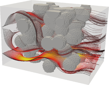
Figure 1: Streamlines in the fluid flow through three-dimensional random model of porous media at porosity $\varphi=0.6$ and tortuosity T=1.15.

Comparison of Eqs. (2) and (4), as well as a research into the literature, reveal the first problem with tortuosity: depending on the context, this term can be related to $T$, $T^{2}$ or even $T^{-1}$ or $T^{-2}$ Bear (1972); Dullien (1992); Clennell (1997); Araújo et al. (2006). The second problem is that a link between the tortuosity defined as an average elongation of fluid paths, as in Eq. (2) (see Fig. 1), and the tortuosity defined as a retardation factor, as in Eq. (4), is well-defined only for the capillary model. It is not clear that a similar correlation exists for arbitrary porous media. The third problem is an imprecise definition of the effective fluid path length ($L_{\mathrm{eff}}$) in Eq. (2). In real porous media flow paths are extremely complicated, as the fluid fluxes continuously change in sectional area, shape and orientation as well as branch and rejoin, and this observation led several researchers Dullien (1992) to believe that $L_{\mathrm{eff}}$ can be defined only in relatively simple network models, which, however, can be analyzed without this notion. The fourth problem is that the Carman-Kozeny formula, Eq. (1), actually defines the product $\beta T^{2}$ (known as the Kozeny constant) and if the tortuosity could not be measured for general porous media, the shape factor and hydraulic tortuosity would become essentially indeterminate quantities, rendering the tortuosity a ‘fudge factor’ used to fit the model to the experimental data Dullien (1992); Tye (1982).

In this paper we discuss some recent achievements in solving the above-mentioned problems. In particular, we show some applications and implications of our recent formula for the tortuosity Duda et al. (2011)

$$T=\frac{\langle u\rangle}{\langle u_{x}\rangle},$$ (5)

where $\langle u\rangle$ is the average magnitude of the intrinsic velocity over the entire system volume and $\left<u_{x}\right>$ is the volumetric average of its component along the macroscopic flow direction.

2 Solution to the fluid flow problem

In order to compute the tortuosity defined with Eq. (5) one has to know the steady state velocity field. This may be accomplished either experimentally, e.g. by using the particle image velocimetry methods Cassidy et al. (2005); Lachhab et al. (2008); Morad and Khalili (2009), the magnetic resonanse imaging Irwin et al. (1999); Werth et al. (2010) or numerically, by finding the solution to the Navier–Stokes equations in the pore space of a porous medium.

Here we take the numerical approach. We use the lattice Boltzmann method (LBM) Succi (2001). In this method, which originates from the kinetic theory of gases and the lattice gas automata models McNamara and Zanetti (1988), the fluid is modeled as consisting of fictive particles propagating and colliding on a discrete lattice. Space, time and velocities are all discrete, with space usually discretized into a regular grid, time discretized into equal intervals, and velocities restricted to just a few vectors $\mathbf{c}_{i}$ related to the geometry of the lattice. The state of the system is fully characterized by distribution functions $f_{i}(\mathbf{x},t)\in[0,1]$ defined for each lattice node $\mathbf{x}$, discrete time $t$, and $\mathbf{c}_{i}$. They can be interpreted as being proportional to the number of particles that at time $t$ are at node $\mathbf{x}$ and have velocity $\mathbf{c}_{i}$. It was shown that solving the LBM model leads to the solution of the incompressible Navier-Stokes equations Luo (2000).

2.1 Sailfish and tortuosity computation

All our numerical computations were performed using the Sailfish library Sailfish (2012), which is an implementation of the LBM method running on graphics processing units (GPUs), an emerging platform for high-performance computing. Sailfish is an open-source project written in the Python programming language, and hence is a highly customisable software. In particular, implementation of Eq. (5) in Sailfish is trivial and consists of just a few lines of code.

3 Tortuosity computation

A general discussion of Eq. (5), its relation to Eq. (2) and conditions of applicability can be found in Duda et al. (2011). Here we use the fact that the LBM method uses a regular (i.e. cubic) mesh. This allows to approximate Eq. (5) with

$$T=\frac{\sum_{\mathbf{r}}u(\mathbf{r})}{\sum_{\mathbf{r}}u_{x}(\mathbf{r})},$$ (6)

where $\mathbf{r}$ runs through all lattice nodes. Note that this simple formula can be used not only in numerical studies, but also for the data obtained experimentally.

In subsequent subsections we test how Eq. (6) behaves for flows in various geometries of increasing complexity.

3.1 Inclined channel

The simplest model of a porous medium approximates it as a bunch of straight pipes, each inclined at an angle $\alpha$ to the macroscopic flow direction. In this case all streamlines are of the same length and Eq. (2) yields $T=1/\cos\alpha$.

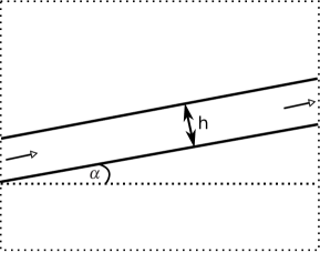
Figure 2: A channel rotated by an angle $\alpha$.

We constructed two two-dimensional (2D) configurations of an inclined channel of height h, with $h=5$ and $20$ lattice units (l.u.) (see Fig. 2). We used the mesh resolution $240\times 800$ (l.u.), set the lattice kinematic viscosity at $\nu=0.01$ and assumed the lattice velocity $u_{\mathrm{max}}=0.02$ as the maximum value of the developed velocity profile at the inlet and outlet. Starting from $\alpha=0$, we succesively rotated the channel preserving its width. For each inclination angle the steady state was found using the LBM method and then the tortuosity was calculated from Eq. (6). The results are depicted in Fig. 3.

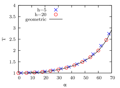
Figure 3: Hydraulic tortuosity $T$, Eq. (5), in a channel of height $h$ (lattice units) rotated by an angle $\alpha$. The solid line shows the geometric tortuosity $1/\cos\alpha$.

They agree well with the values expected from geometric considerations even for a narrow channel of height h=$5$ l.u. (the relative difference does not exceed 5%). Small errors observed in our simulations stem from discretization errors and the staircased approximation of the channel boundaries in the LBM method Matyka et al. (2012), which results in $T$ being slightly overestimated. These errors decrease with an increasing value of $h$.

3.2 U-shaped channel

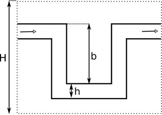
Figure 4: The U-shaped channel with a step depth $b$.

Next, we constructed a U-shaped channel geometry (see Fig. 4). The mesh resolution was set at $L\times H=300\times 200$ (l.u.), and we assumed $\nu=0.01$ and $u_{\mathrm{max}}=0.01$. We started from the step depth $b=0$ and increased it until $b=H/2$. For each $b$ two channel heights, $h=5$ and $h=20$ (l.u.) were investigated. In this geometry the geometric tortuosity $T_{\mathrm{g}}=(L+2b)/L$.

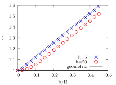
Figure 5: Hydraulic tortuosity, $T$, computed using Eq. (5) in a U-shaped channel as a function of the relative step depth $b/H$ for two channel heights $h$ (lattice units). The solid line represents the geometric tortuosity for the same system.

Comparison of the tortuosity determined from Eq. (6) with $T_{\mathrm{g}}$ for various values of $b$ and $h$ is shown in Fig. 5. As expected, a linear dependency of geometric and hydraulic tortuosities on $b$ is visible, but a deviation of $T$ from $T_{\mathrm{g}}$ at larger channel depths $b$ is also noticeable. To understand this effect we analyzed the flow streamlines for this systems (data not shown) and observed that they follow the geometry nicely only at the straight parts of the channel. At corners, however, a tendency of flow paths to seek a shorter path is visible. This leads to the hydraulic tortuosity $T$ being smaller than the geometric one, as shown in Fig. 5. This effect is more visible for larger $h$, as in this case the corner deformation is more pronounced.

3.3 Two-dimensional overlapping circles

The next model we considered was a 2D system in which the porous matrix was modeled by circles that were free to overlap. We used a $900\times 600$ mesh at which we randomly deposited monosized circles of radius $r=10$ l.u. No-slip boundary conditions were imposed on the top and bottom walls and periodic boundary conditions were assumed at the inlet and outlet. The flow was driven by an external force field whose magnitude was chosen so that the Reynolds number $\mathrm{Re}<1$ (creeping flow). The circles were deposited only in the central, $600\times 600$ (l.u.) area of the mesh, see Fig. 6.

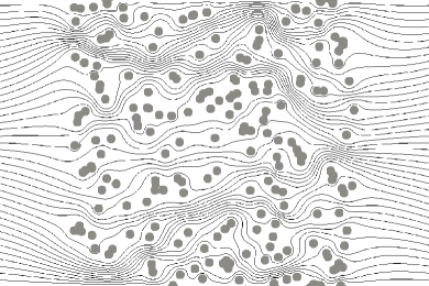
Figure 6: Flow streamlines in a realization of a two-dimensional model of a porous medium built of overlapping circles of radius $R=10$ (l.u.) at porosity $\varphi=0.85$. The tortuosity computed using Eq. (6) is $T=1.13$.

The remaining space was kept empty to minimize the influence of inlet and outlet boundary conditions. We ran the simulation for 40 000 steps until the steady state was reached and used Eq. (6) to compute the tortuosity. As seen in Fig. 6, the flow streamlines in this model can be quite complex and “tortuous”.

In our previous studies Matyka et al. (2008); Koza et al. (2009) we considered a similar model in which the porous matrix was modeled by overlapping squares and the tortuosity was computed directly as an average over streamline lengths. We found that in that model the relation between tortuosity and porosity could be approximated by Comiti’s and Renaud’s logarithmic formula Comiti and Renaud (1989)

$$T=1-p\ln\varphi$$ (7)

with a fitting parameter $p=0.77$. The dependency of the tortuosity on the porosity in the present model of overlapping circles is shown in Fig. 7.

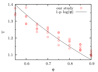
Figure 7: Tortuosity as a function of porosity in the two-dimensional model of overlapping circles computed using Eq. (5). Symbols are our numerical results, the solid line is the best fit to Eq. (7).

We fitted the data to Eq. (7) and found a good agreement for $p\approx 0.67$.

3.4 Three-dimensional overlapping spheres

As the final test of Eqs. (5) and (6) we used them to find the flow tortuosity in a three-dimensional (3D) model of overlapping spheres. The geometry was constructed similarly to the two-dimensional case described above. A regular grid of $90\times 90\times 90$ nodes was generated and freely overlapping spheres of radius 10 l.u. were deposited in it to reach the desired porosity value. The system was assumed periodic in the $x$ direction and no-slip walls were imposed at the four remaining walls. We ran the LBM simulation for 10 000 time steps to reach the steady state and then computed the tortuosity from Eq. (6).

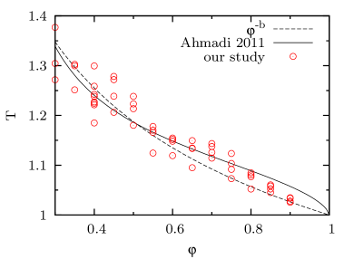
Figure 8: Tortuosity, Eq. (5), as a function of porosity in a three-dimensional model of overlapping spheres. Open symbols are our numerical results, the solid line is the best fit to Eq. (8), and the dashed line is the best fit to $T=\varphi^{-b}$ with $b\approx 0.25$.

The tortuosity-porosity dependence in our 3D model is shown in Fig. 8 (circles). The solid line in this figure depicts a formula that was recently derived analytically for a very similar model Ahmadi et al. (2011); Nemati Hayati et al. (2012),

$$T=\sqrt{\frac{2\varphi}{3\left[1-B(1-\varphi)^{2/3}\right]}+\frac{1}{3}},$$ (8)

where $B$ is a constant that depends on the shape of the obstacles and the lattice used. The main difference between our model and that studied in Ahmadi et al. (2011); Nemati Hayati et al. (2012) is that we distribute the spheres at random positions and allow them to overlap, whereas Eq. (8) was derived for regular arrangements of impermeable, non-overlapping objects of essentially arbitrary shape. Assuming that Eq. (8) can be also used for non-regular arrangements of spheres, we fitted our data to this formula using $B$ as a free parameter. This gave $B\approx 1.09$, which is a bit smaller than $B\approx 1.209$ derived in Ahmadi et al. (2011) for the cubic packing of spheres. As seen in Fig. 8, our results are in good agreement with Eq. (8) in the whole range of porosities.

Archie’s law Archie (1942); Clennell (1997)

$$T_{\mathrm{el}}=\varphi^{-n},$$ (9)

is another formula for the tortuosity-porosity relation, often used for retardation tortuosities, especially the electrical and diffusional one. Together with Eqs. (2), (3), Archie’s law suggests $T=\varphi^{-b}$ with $b=(n-1)/2$. Our data can be fitted to this formula with $b\approx 0.25$, see Fig. 8, which yields $n\approx 1.5$, which lies in the range $1.3\leq n\leq 3$ reported in Clennell (1997). A more detailed analysis, involving a bigger number of larger systems, is necessary to verify which of the equations should be applied to this model, and whether Eq. (8) actually applies to non-regular arrangements of obstacles.

4 Discussion and outlook

We have presented several applications of our recently introduced method of calculating the tortuosity defined as a measure of the average elongation of fluid streamlines Duda et al. (2011). Starting from a simple model of an inclined channel, through a U-shaped channel, and ending at complex 2D and 3D geometries, we found a very good agreement of this method with other methods serving the same purpose. However, the main advantage of our method is that it does not require to find any streamlines, which is a complicated, time-consuming and error-prone task, especially in realistic 3D geometries. Instead, it allows to calculate the streamline tortuosity directly from the velocity field. Not only does this simplify numerical studies of this quantity, but should also greatly simplify experimental measurements of $T$.

To summarize, there are several advantages of calculating the streamline tortuosity using the method of Ref. Duda et al. (2011). First, the formula is simple and flexible, allowing to compute the tortuosity of practically any hydrodynamical fluid flow system in which the velocity field can be determined, whether numerically, analytically or experimentally. Second, this method solves the problem of the very existence of tortuosity as an average elongation of fluid paths. As a consequence, one can concentrate on the physical significance of this quantity, including finding its relation with numerous “tortuosities” defined as transport retardation factors. In this context it is interesting to notice that since the streamline tortuosity can be expressed as the ratio of the average fluid velocity magnitude to the average fluid velocity along the macroscopic flow direction, it turns out to be closely related to one of the most fundamental physical phenomena—momentum transfer. Third, this formula can be applied to other forms of transport in porous media, e.g. to diffusion or electric current Duda et al. (2011). Fourth, our formula can be used to flows in the fractal-like Andrade et al. (2007) or ramified structures Andrade et al. (1998); Almeida et al. (1999), sytems which are not considered porous. For example, one could compute hemodynamical tortuosity in the flow through human artery system, in which a fundamental difference between the geometrical and hydraulic tortuosities may be of profound importance for medical diagnosis of arterial diseases Wolf et al. (2001).

References

- Carman (1937) P. C. Carman, Trans. Inst. Chem. Eng. 15, 150–166 (1937).
- Bear (1972) J. Bear, Dynamics of Fluids in Porous Media, Elsevier, New York, 1972.
- Dullien (1992) F. A. L. Dullien, Porous media: fluid transport and pore structure, Academic Press, New York, 1992.
- Clennell (1997) M. B. Clennell, Geol. Soc. Spec. Publ. 122, 299–344 (1997).
- Araújo et al. (2006) A. D. Araújo, W. B. Bastos, J. S. Andrade, Jr., and H. J. Herrmann, Phys. Rev. E 74, 010401(R) (2006).
- Tye (1982) F. L. Tye, Chemistry and Industry 182, 322–326 (1982).
- Duda et al. (2011) A. Duda, Z. Koza, and M. Matyka, Phys. Rev. E 84, 036319 (2011).
- Cassidy et al. (2005) R. Cassidy, J. MccLoskey, and P. Morrow, Geological Society, London, Special Publications 249, 115–130 (2005).
- Lachhab et al. (2008) A. Lachhab, Y. Zhang, and M. Muste, Ground Water 46, 865–872 (2008).
- Morad and Khalili (2009) M. Morad, and A. Khalili, Experiments in Fluids 46, 323–330 (2009).
- Irwin et al. (1999) N. Irwin, S. Altobelli, and R. Greenkorn, Magnetic Resonance Imaging 17, 909 – 917 (1999).
- Werth et al. (2010) C. J. Werth, C. Zhang, M. L. Brusseau, M. Oostrom, and T. Baumann, Journal of Contaminant Hydrology 113, 1 – 24 (2010).
- Succi (2001) S. Succi, The Lattice Boltzmann Equation for Fluid Dynamics and Beyond, Clarendon Press, New York, 2001.
- McNamara and Zanetti (1988) G. R. McNamara, and G. Zanetti, Phys. Rev. Lett. 61, 2332–2335 (1988).
- Luo (2000) L.-S. Luo, Phys. Rev. E 62, 4982–4996 (2000).
- Sailfish (2012) Sailfish, http://sailfish.us.edu.pl/ (2012).
- Matyka et al. (2012) M. Matyka, Z. Koza, and Ł. Mirosław (2012), arXiv:1203.3078.
- Matyka et al. (2008) M. Matyka, A. Khalili, and Z. Koza, Phys. Rev. E 78, 026306 (2008).
- Koza et al. (2009) Z. Koza, M. Matyka, and A. Khalili, Phys. Rev. E 79, 066306 (2009).
- Comiti and Renaud (1989) J. Comiti, and M. Renaud, Chem. Eng. Sci. 44, 1539–1545 (1989).
- Ahmadi et al. (2011) M. M. Ahmadi, S. Mohammadi, and A. N. Hayati, Phys. Rev. E 83, 026312 (2011).
- Nemati Hayati et al. (2012) A. Nemati Hayati, M. M. Ahmadi, and S. Mohammadi, Phys. Rev. E 85, 036310 (2012).
- Archie (1942) G. Archie, Trans. Am. Inst. Min., Metall. Pet. Eng. 146, 54–62 (1942).
- Andrade et al. (2007) J. S. Andrade, A. D. Araújo, M. Filoche, and B. Sapoval, Phys. Rev. Lett. 98, 194101 (2007).
- Andrade et al. (1998) J. S. Andrade, A. M. Alencar, M. P. Almeida, J. Mendes Filho, S. V. Buldyrev, S. Zapperi, H. E. Stanley, and B. Suki, Phys. Rev. Lett. 81, 926–929 (1998).
- Almeida et al. (1999) M. P. Almeida, J. S. Andrade, S. V. Buldyrev, F. S. A. Cavalcante, H. E. Stanley, and B. Suki, Phys. Rev. E 60, 5486–5494 (1999).
- Wolf et al. (2001) Y. G. Wolf, M. Tillich, W. A. Lee, G. D. Rubin, T. J. Fogarty, and C. K. Zarins, Journal of Vascular Surgery 34, 594–599 (2001).