Intensity and polarization of the atmospheric emission at millimetric wavelengths at Dome Concordia

Abstract

Atmospheric emission is a dominant source of disturbance in ground-based astronomy at millimetric wavelengths. The Antarctic plateau is recognized to be an ideal site for millimetric and sub-millimetric observations, and the French/Italian base of Dome Concordia is among the best sites on Earth for these observations. In this paper we present measurements at Dome Concordia of the atmospheric emission in intensity and polarization at $2\ mm$ wavelength, one of the best observational frequencies for Cosmic Microwave Background (CMB) observations when considering cosmic signal intensity, atmospheric transmission, detectors sensitivity, and foreground removal. Using the BRAIN-pathfinder experiment, we have performed measurements of the atmospheric emission at $150\ GHz$. Careful characterization of the air-mass synchronous emission has been performed, acquiring more that 380 elevation scans (i.e. “skydip”) during the third BRAIN-pathfinder summer campaign in December 2009/January 2010. The extremely high transparency of the Antarctic atmosphere over Dome Concordia is proven by the very low measured optical depth: $<\tau_{I}>=0.050\pm 0.003\pm 0.011$ where the first error is statistical and the second is systematic error. Mid term stability, over the summer campaign, of the atmosphere emission has also been studied. Adapting the radiative transfer atmosphere emission model am to the particular conditions found at Dome Concordia, we also infer the level of the precipitable water vapor (PWV) content of the atmosphere, notoriously the main source of disturbance in millimetric astronomy ($<PWV>=0.77\pm 0.06\pm^{0.15}_{0.12}\ mm$). Upper limits on the air-mass correlated polarized signal are also placed for the first time. The degree of circular polarization of atmospheric emission is found to be lower than 0.2% (95%CL), while the degree of linear polarization is found to be lower than 0.1% (95%CL). These limits include signal-correlated instrumental spurious polarization.

1 Introduction

Fast growing fields in millimetric astronomy are the study of the Cosmic Microwave Background (CMB) polarization and the measurement of polarized emission from interstellar dust. In particular, a curl component (B-modes) of the CMB polarization from the predicted inflationary expansion of the universe earlier in time may be present. The theorized signal depends on the energy of the inflationary field, as measured by the tensor-to-scalar ratio r, and is so low that exquisite sensitivity and control of systematic effects are necessary to attempt these kind of observations.

Atmospheric emission is one of the dominant sources of disturbance for ground-based CMB experiments and for millimetric and sub-millimetric astronomy in general. In addition to continuum emission at the frequencies of our interest, there are also the roto-vibrational emission lines of $O_{2}$ (at around $60\ GHz$ and $119\ GHz$) and $H_{2}O$ (at $22\ GHz$ and $183\ GHz$). Dry and high altitude observation sites are chosen to mitigate the problem. The French/Italian scientific base of Dome Concordia on the Antarctic plateau ($75^{\circ}06^{\prime}$ South, $123^{\circ}24^{\prime}$ East, at $3233\ m$ aside see level, http://www.concordiabase.eu/) is one of the best observational sites on Earth for millimetric observations. Site testing at Dome C has proven its observational quality at different wavelengths (see e.g. Tremblin et al. (2011); Gredel (2010); Lawrence et al. (2004); Aristidi et al. (2009); Calisse et al. (2004)) although only preliminary measurements were performed at millimeter wavelengths Valenziano et al. (1999). $150\ GHz$ is among the best observational frequencies for ground based CMB experiments in terms of cosmic signal intensity, atmospheric transmission, detectors sensitivity and foreground removal.

The BRAIN-pathfinder experiment Masi et al. (2005); Polenta et al. (2007) has undergone its third Antarctic campaign from the French/Italian scientific base of Dome Concordia. The first two campaigns were dedicated to instrument fielding, while the 2009-2010 austral summer campaign was dedicated to continuous observations of the atmospheric emission and site testing. This paper is structured as follows: in $\S$2 we introduce the BRAIN-pathfinder instrument, in $\S$3 we describe the observations; in $\S$4 we present the data and the analysis and in $\S$5 we give the results in terms of intensity and polarization.

2 BRAIN-pathfinder: the instrument

The BRAIN-pathfinder was designed as a prototype instrument for a challenging project of bolometric interferometer. The BRAIN collaboration has been combined with the Millimeter-wave Bolometric Interferometer (MBI) Tucker et al. (2008) collaboration to form the QUBIC collaboration. The BRAIN-pathfinder was devoted to site and logistics testing for the QUBIC experiment The QUBIC collaboration (2011), that we aim to install at Dome Concordia in 2013. The BRAIN-pathfinder instrument is described in detail elsewhere Masi et al. (2005); Polenta et al. (2007); Masi et al. in prep . Nevertheless, we here report a brief description of the instrumental setup for completeness.

The BRAIN-pathfinder comprises of a two-channel bolometric receiver coupled to two off-axis ($40$ and $60\ cm$ diameter) parabolic mirrors, tiltable around the optical axis. The whole instrument is mounted on an azimuth plane, making the instrument an Alt-Az double telescope. The first in its kind, our bolometric receiver is cooled by a dry-cryostat with a Sumitomo Pulse Tube cryocooler, allowing us to keep an intermediate stage at $30\ K$ and a main plate at $3\ K$. Quasi-optical filters, JFET boards and shields are kept at $30\ K$ with JFET amplifiers attached to their PCB through weak thermal connections in their fiberglass supports. Further filters, radiation collecting horns and further shields are kept at $3\ K$ with an ${}^{3}He-^{4}He$ refrigerator that keeps the bolometers at 310mK during observations.

One of the two channels (channel 1) measures the anisotropy of the emission of the sky, while the second one (channel 2) sees the sky through an ambient-temperature, rotating sapphire Quarter Wave Plate (QWP), and a steady wire grid polarizer. The presence of the rotating QWP makes this second detector inherently sensitive to linear and circular polarization. In an ideal case, the power hitting channel 2 is thus Polenta et al. (2007):

$$\centering W=\frac{1}{2}[I_{in}+Q_{in}\frac{1+cos(4\omega t)}{2}+U_{in}\frac{sin(4\omega t)}{2}+V_{in}sin(2\omega t)]\@add@centering$$ (1)

where $I_{in}$, $Q_{in}$, $U_{in}$, and $V_{in}$ and the Stokes parameters of the incoming radiation, $\omega$ is the mechanical angular speed of the QWP. From equation 1 it is clear that an incoming polarized radiation is modulated by the rotating QWP at a frequencies twice or four times the mechanical frequency, depending whether the polarization is circular or linear.

We use the control and read-out electronics, as well as the control software, originally developed for the Planck High frequency Instrument Lamarre et al. (2010) and for its ground based calibrations. Its angular resolution on the sky is $1^{\circ}$. A double back-to-back horn and the quasi-optical filters set the average observational frequency at $150\ GHz$, with $36\ GHz$ FWHM bandwidth. Detailed measurements of the bandpass have been performed combining data obtained with a high throughput Fourier Transform Spectrometer Schillaci (2010) and a Vector Network Analyzer in order to characterize the transmission curve especially on the low frequency end of the band-pass, where the molecular Oxygen line emission becomes brighter.

3 Observations

Observations were taken during the 2009-2010 austral summer Antarctic campaign. As opposed to a CMB experiment, for which one should choose an observational strategy aiming at minimizing the atmospheric effects (see eg. Chiang et al. (2010), Castro et al. (2009)), we have chosen an observational strategy able to highlight the atmospheric contribution. Here we present a full characterization of the air-mass dependence of the atmospheric intensity and polarized emission, obtained by performing elevation scans (i.e. skydips) by leaving the azimuth constant and scanning the elevation from the zenith to $35$ degrees above the horizon.

Elevation scans were done in a so called “fast scan” mode by acquiring the sky signal while the telescope continuously samples different elevation angles. The scan speed has been chosen as high as possible, in order to mitigate the $1/f$ noise present in the data arising both from detector instability and (mainly) from the slow variation of the atmospheric emission. At the same time we set the scan speed to be able to acquire multiple QWP rotations in one single telescope beam. We tested different QWP and scan speeds and, trading off instrumental constrains and observational needs. We set the QWP rotational frequency at $1.56\ Hz$ (corresponding to $3.13\ Hz$ and $6.26\ Hz$ respectively for circular and linear polarization modulation frequencies) for approximately half of the measurements and at $2.09\ Hz$ (corresponding to $4.17\ Hz$ and $8.35\ Hz$ respectively for circular and linear polarization modulation frequencies) for the rest of the time. A scan speed of $1^{\circ}/s$ thus allows at least three or six polarized modulation periods per telescope beam. With these settings, a full scan completes in less than a minute, a short enough time to mitigate slow signal variation arising from atmospheric emission.

In order to reduce the field of view vignetting, to overcome detector and read-out non-linearity, and to optimize the detectors dynamics, we have chosen not to use a warm reference load for skydip measurements. This forces us to make some assumptions if we want to do absolute calibration of the data (see section 4). On the other hand, it allows us to directly analyze polarization data relatively to the intensity emission, with no need of any reference signal.

We have collected 383 skydips. About 12% of the skydips were discarded because of corrupted data or due to large atmospheric fluctuations. About 76% of the analyzed skydips were acquired changing the elevation from the zenith to $35$ degrees above the horizon (long skydip) while the remaining 24% were limited to $60$ degrees above the horizon (short skydip), in order to keep the Sun always at an angle larger than $30$ degrees from the field of view. Most of the reported results have been extracted from the analysis of the long skydips, although the short ones have been useful for cross checks.

4 Data reduction and analysis

The skydip technique Dicke et al. (1946) is a well investigated method to study the atmospheric emission (see e.g. Dragovan et al. (1990), Archibald et al. (2002)). During a skydip we expect the acquired signal to respond to the air-mass as in the following:

$$\centering S=off+C\cdot T_{0}\cdot[1-exp(-x\cdot\tau_{I})]\@add@centering$$ (2)

where $S$ is the acquired signal in ADC units, $off$ is an instrumental offset in ADC units, $C$ is the calibration factor in ADC/K units, $T_{0}$ (in K) is the equivalent temperature of the atmosphere, $\tau_{I}$ is the sky opacity and $x=sec(z)$ is the air-mass with the zenithal angle $z=90^{\circ}-elevation$.

One of the features in our data is the presence in the time stream of a periodic signal at a frequency of around $1\ Hz$ due to the pulses of the Pulse Tube cryocooler. In fact, the experimental effort spent to reduce the system vibration has drastically reduced but not completely eliminated the effect of the pulses on the high impedence bolometers, that are intrinsically microphonic. This does not affect the high signal-to-noise skydip measurements we are analyzing in this paper; nevertheless we have decided to filter out from our data this well defined imprint, in order to avoid biases in the skydip fits. We have performed several tests, both in time and in Fourier space and we finally decided to use a multiple Notch filter to remove the main pulse frequency and its harmonics.

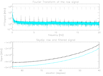
Figure 1: Data acquired during one skydip. The plot on the top shows the Fourier transform of the raw data (black, solid), the used multiple Notch filter (black, dotted) and the filtered data (cyan, solid, overplotted on the data). The plot on the bottom shows a raw skydip (black), and a filtered skydip (cyan) offset by 60000 Analog to Digital Units (ADU).

In figure 1 we show filtered and unfiltered signals (and their Fourier transforms), in engineering units, acquired during one skydip.

While for channel 1 we have only (Notch-) filtered out the Pulse Tube $1\ Hz$ signal, in order to retrieve signal intensity information from channel 2 we have to account for the presence of the rotating QWP in front of it. We have thus applied a low-pass filter, with cut-off frequency at $1\ Hz$, to remove any higher frequency signal due to the rotating QWP that could modulate linear and circular polarized signal. Dedicated band-pass filters have then been applied to retrieve polarization information (see section 5.3 for details).

We have performed a likelihood analysis and chi square minimization to optimize secant-law fits on each of the acquired skydips. We have verified the linearity of the dependence of the signal as a function of the air-mass. This is verified only in the case of high transparency of the atmosphere:

$$\centering S=P_{1}+P_{2}\cdot exp(-P_{0}\cdot x)\simeq P_{1}+P_{2}-P_{2}\cdot P_{0}\cdot x=A^{I}-B^{I}\cdot x\@add@centering$$ (3)

where $A^{I}=P_{1}+P_{2}$ and $B^{I}=P_{2}\cdot P_{0}$ are the fitted parameters.

Comparing equation 2 and 3 we determine the sky opacity:

$$\centering\tau_{I}=-B^{I}/(C\cdot T_{0})\@add@centering$$ (4)

where the calibration factor $C$ has been determined by using laboratory absolute reference loads cooled at liquid Nitrogen temperature (i.e. $77\ K$), careful measurements of the bolometer efficiency, as well as the daily electrical responsivity measurements performed during observations through the measurements of the detector $I-V$ curve. The temperature $T_{0}$ was determined by integrating the temperature, pressure and humidity profiles obtained by daily measurements with atmospheric radio-sound balloons flying up to an altitude of $24000\ m$, collecting data with $\Delta h\sim 10\ m$ altitude sampling. In particular, these data, combined with continuous ground temperature measurements at the time of the skydip, and after integration of the atmospheric emission contribution over the altitude for each of our scans, allowed us to recover $T_{0}$ using radiative transfer.

Our model for atmosphere emission is made by two different parts: in order to reconstruct the circularly polarized $O_{2}$ signals we use the model described in Spinelli et al. (2011). This model can be used to estimate also Stokes paramaters I,Q and U. In order to deal with a complete dry-air model, together with a water vapor column, we used the am model Paine et al. (2011). The am model uses updated spectroscopic parameters and is readily available, very well supported, and documented. We have made day-by-day estimates of the atmospheric emission using radio sounds, properly resampled to build am configuration files. The resulting brightness temperature is then averaged over the frequency bandpass of BRAIN-pathfinder channels, after accurate laboratory bandpass reconstruction, to obtain the power delivered to our detectors. We find a linear scaling relation between the precipitable water vapor (PWV), or the integrated optical depth $\tau$, and the brightness temperature $T_{b}$ in our bandpass, that is:

$$\centering T_{b}=Q+M\cdot PWV,\@add@centering$$ (5)

where $M_{ch1}=(6.6\pm 0.3)K/mm$, $M_{ch2}=(5.4\pm 0.3)K/mm$, $Q=(4.2\pm 0.2)K$ with PWV expressed in mm. Not surprisingly, the two M coefficients are different, since our bandpasses is strongly suppressed towards the 118 GHz $O_{2}$ line, while their high frequency wings pick up with small (but not negligible) and different efficiency a residual signal from the 183 GHz $H_{2}O$ line. The intercept Q is sensitive to the dry-air component, mainly to $O_{2}$, whose tail is observed with the same efficiency by our detectors.

In order to account for polarized emission one has to consider magnetic field direction and intensity. We have estimated these for the Austral summer 2009/2010, at Dome C, by means of the International Geomagnetic Reference Field (IGRF) model was used. The day-by-day variation in atmospheric conditions produces a small uncertainty on the oxygen polarized and unpolarized brightness temperature computed through their model (seasonal variations and magnetic storms being definitely more relevant). In particular, in the specific case of the BRAIN campaign, the absolute uncertainty on $O_{2}$ modeled signals is of the order of a few $\mu$K and a few mK, respectively, for the V and I maps. Both these uncertainties are negligible with respect to the one associated with $H_{2}O$ emission estimates, which is of the order of some tens of mK. This last one is driven mainly by the day-by-day scatter of atmospheric parameters.

We found the uncertainty derived from the fits negligible with respect to the estimated uncertainty derived from the calibration procedure. This can be as high as 23% and should be treated as a systematic error. It dominates over all other uncertainties. Calibration uncertainties proportionally propagate to the opacity determination, while we produced monte-carlo simulations in order to estimate PWV uncertainties.

In figure 2 we report best fit curves obtained over the calibrated skydips collected during the campaign for both channels.

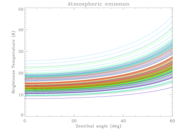
Figure 2: Collection of best fit curves obtained over the calibrated skydips collected during the 2009-2010 summer campaign.

5 Results

5.1 Sky opacity

The distribution of the sky opacities measured during the campaign can be seen in the histogram in figure 3. The cyan (light) histogram is derived from channel 2 measurements while the black (dark) histogram (summed and positioned on top of the cyan one) is derived from channel 1 measurements. The measurements from both channels result in $\tau_{I}$ values centered around an average value $<\tau_{I}>=0.050$, with a median of $\tau_{I}^{m}=0.048$ and statistical error on each measurement of 7%. This corresponds to an average transmission of $95\%$. Although all the measurements have been taken with clear sky, we should stress that the reported results reflect a wide variety of weather conditions and only bad weather situations (i.e. covered sky, although rare at Dome C) have been discarded from our analysis.

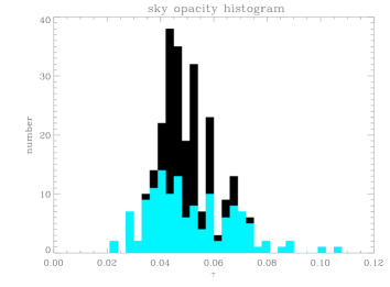
Figure 3: Histogram of measured sky opacity. The cyan (light) histogram is obtained from channel 2 measurements; the black (dark) histogram is obtained from the collection of channel 1 measurements and is positioned over channel 2 data.

In figure 4 we show the atmospheric transmission measurements along the whole campaign. In figure 5 we show the same measurements averaged on day by day basis. Transmission seems to be fairly constant along the campaign, with a possible general trend to decrease in the middle of the campaign and a rise back at the end of it. Error bars in figure 5 reflect the variability within each day. This parameter has to be taken into account when considering measurements with thermal detectors like transition edge sensor (TES) bolometers (as those planned for the QUBIC experiment) when accounting for load variation on the bolometers themselves, and TES plus superconducting quantum interference devices (SQUIDs) working point tuning. We estimate a relative average variation, on a daily basis, of 0.9 per cent, consistent with one single tuning procedure per day needed Battistelli et al. (2011). Peaks of a few per cent have also been observed in limited cases. This would require tuning procedures to be run more than once a day. In figure 6 we show the transmission measured within the day. We have averaged over skydips acquired less than 2 hours apart on different days. In order to reduce the scatter caused by different days of observations, we have normalized each measurement to the average daily measurements and multiplied by the overall average transmission. Also in this case the trend seems to be fairly constant, with a slight decrease in the middle of the day due to the increase of elevation of the Sun.

Figure 4: Atmospheric transmission during the 2009-2010 campaign. Statistical uncertainties only are shown in this graph.

Figure 5: Atmospheric transmission during the 2009-2010 campaign. In this plot we averaged over the skydip acquired during the same day. This shows the general trend of the sky transmission during the campaign.

Figure 6: Atmospheric transmission during the 2009-2010 campaign. In this plot we averaged over the skydip acquired less than 2 hours apart, each measurement being normalized by the average daily transmission, relative to (multiplied by) the overall average transmission on the campaign. This shows the general trend of the sky transmission during the day.

5.2 Precipitable water vapor content

We have used am model Paine et al. (2011) to infer, from our sky opacity measurements, the characteristics in terms of PWV of the atmosphere over Dome C during our measurements. This model as been tailored and configured for Dome C conditions and allows us to exploit balloon data taken during the campaign, in view of the interpretation of BRAIN data. We have found a scaling law between a photometric quantity (the brightness temperature) and an atmospheric parameter (PWV), thus removing possible degeneracies in our analysis.

In figure 7 we show the histogram of the Precipitable Water Vapor content obtained from our skydips. These are obtained by fitting our calibrated skydips over the simulated template and by only accounting for the brightness temperature change over the skydip, and not its offset, and checking the zenith brightness temperature for consistency.

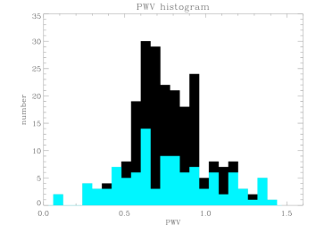
Figure 7: Histogram of the derived Precipitable Water Vapor Content on the atmosphere. The cyan (light) histogram is obtained from channel 2 measurements; the black (dark) histogram is obtained from the collection of channel 1 and channel 2 measurements.

During the BRAIN-pathfinder 2009-2010 campaign we find an average PWV of $<PWV>=0.77\ mm$, with statistical errors on each measurement of $\pm 0.06\ mm$ and calibration uncertainties of ${}^{+0.15}_{-0.12}\ mm$. We find a median of $PWV^{m}=0.75\ mm$, an average 25th percentile of $PWV^{25th}=0.49\ mm$ and an average 75th percentile of $PWV^{75th}=1.1\ mm$. This level of PWV content is in good agreement with those measured in 2003-2005 and 2005-2009 with radio-sounding measurements Tomasi et al., (2006); Tomasi et al. (2011) and with those measured by Tremblin et al. (2011) at 1.5 THz. Nevertheless, we should stress that the main results of our measurements are obtained by directly sampling the same spectral bandwidth of scientific interest and are thus free from model dependent bias.

5.3 Polarization

As previously mentioned, channel 2 of the BRAIN-pathfinder measures sky emission through a rotating QWP followed by a wire-grid polarizer. During observations we rotated the QWP at several different speeds. For instrumental, environmental, and noise reasons we set its physical rotational frequency at $\nu_{QWP}=1.56\ Hz$ ($2.09\ Hz$) for most of our observations. We thus expect any incoming circularly polarized signal to be modulated at $\nu_{C}=2\cdot\nu_{QWP}=3.13\ Hz$ ($4.17\ Hz$) and any incoming linearly polarized signal at $\nu_{L}=4\cdot\nu_{QWP}=6.26\ Hz$ ($8.35\ Hz$) (see eq. 1). The emission of the (ambient temperature) QWP and of the polarizer have been studied using the models presented by Salatino et al. (2011). Our data are affected by an offset modulated both at $\nu_{C}$ and at $\nu_{L}$ that we found to be consistent with the QWP emission as well as the polarizer emission reflected back from the QWP. We should stress that the stability of this emitted signal is critical to retrieve meaningful information from the data. One of the goals of this paper is to provide information on the polarization of the skydip signal. For the present analysis, it is critical to characterize and monitor the stability of our instrument within the average time of a skydip as faster instability will affect the results.

We have demodulated the $\nu_{C}$ and the $\nu_{L}$ signals using band-pass filters for each raw skydip. The extracted signals have thus been treated in the same way as the intensity signal in order to find a possible secant law dependence in the polarized signal of the skydips. Once we have performed secant law fits over the polarized skydips, we can define $\tau_{C}$ and $\tau_{L}$ similarly to $\tau_{I}$:

$$\centering\tau_{C}=-(B^{C})/(C\cdot T_{0}),\@add@centering$$ (6)

$$\centering\tau_{L}=-(B^{L})/(C\cdot T_{0}).\@add@centering$$ (7)

The comparison between the different $\tau$’s enables us to extract polarized information from our skydips and thus an estimation of the air-mass-correlated (or anticorrelated) polarization of atmospheric emission.

In figure 8 we show one of the skydips acquired and analyzed in polarization. Polarization calibration has been performed using local polarized sources placed in the near-field and in the medium-field. We should stress, however, that the derived percentage polarization levels are independent of the calibration and of the determination of the equivalent temperature of the atmosphere. The uncertainty on each of the skydip polarization levels is thus directly derived from the fits. After combining and weight-averaging over all the skydips, we find that both circular and linear polarization of the air-mass correlated signals are consistent with zero, with upper limits such that $S_{C}<0.19\%$ and $S_{L}<0.11\%$ (95%CL), respectively. These results have been confirmed by cross-correlating the measured data with the signals expected from Zeeman splitting and simulated using the model developed in Spinelli et al. (2011). These limits include instrumental systematics and place a tight limit on the QWP plus polarizer stability within the time of the acquired skydips.

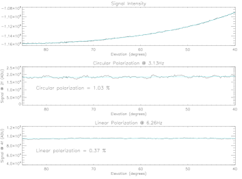
Figure 8: Intensity, linear polarization and circular polarization signal acquired during a single skydip. We plot the acquired data (dark) and the secant law performed fit (light/cyan). We report the derivation of the percentage polarization that can be extracted from this skydip.

6 Conclusions

In this paper we report a detailed site testing of Dome C at $150\ GHz$ and the first limits on the polarized emission of its atmosphere. Dome Concordia is demonstrated to be an exceptional millimetric observational site, in terms of absolute transmission and stability and polarization limits are encouraging as far as spurious polarization and intensity-polarization mixing are concerned. Our opacity measurements have been derived from direct sampling of the frequencies of astronomical interest and are thus free from model-dependent bias. We anticipate that, in most observational conditions, the measured daily stability should enable us to have Transition Edge Sensor Bolometer arrays requiring only a single tuning procedure per day. When comparing our millimetric opacities and in-bandwidth transmissions with those obtained at sub-millimeter wavelengths, the absolute values are one order of magnitude better in terms of transmission and stability. Nevertheless, we should keep in mind that the requirements, in terms of systematic control and stability, for a millimetric B-modes CMB experiment, are such that it is necessary to characterize the atmospheric stability to a high level of precision and our results are very encouraging. Our derived PWV value relies on a model independently developed by the BRAIN collaboration and tailored for Dome C. Our PWV values are consistent with those derived at sub-millimeter wavelenghts Tomasi et al. (2011). In our case, however, radiation is detected through an instrument similar to those aiming to detect CMB polarization, allowing direct monitoring of many systematic effects. Systematic control requirements for a B-mode CMB experiment are so stringent that no instrument, to date, has been able to meet them. The requirement for the instrumental spurious polarization induced from leakage of CMB anisotropies into B-mode polarization is that the leakage should be maintained lower than $10^{-3}$ Bock et al. (2006). This is necessary in order to be able to reach a B-modes signal of the order of $30\ nK$ rms (i.e. Tensor to Scalar ratio r=0.01). In terms of absolute temperature limits, our analysis does not allow us to reach this limit. However, in terms of a relative systematic limit, considering that our 0.1% limit for linear polarization includes spurious polarization due to intensity-to-polarization leakage, our instrument is already satisfying to this requirement.

References

- Archibald et al. (2002) Archibald, E.N., et al., 2002, Montly Notice of the Royal Astronomical Society, 336, 1-13
- Aristidi et al. (2009) Aristidi, E., et al., 2009, Astronomy & Astrophysics, 499, 955-965
- Battistelli et al. (2011) Battistelli, et al., 2008, proceeding of the SPIE, 7020, 702028
- Bock et al. (2006) Bock, J.J., et al., 2006, arXiv:astro-ph/0604101
- Calisse et al. (2004) Calisse, P., et al., 2004, Publications of the Astronomical Society of Australia, 21, 256-263
- Castro et al. (2009) Castro, P.G., et al., 2009, Astrophysical Journal, 701, 2, 857-864
- Chiang et al. (2010) Chiang, H.C., et al., 2010, Astrophysical Journal, 711, 2, 1123-1140
- Dicke et al. (1946) Dicke, R. H., et al., 1946, Physical Review, 70, 5-6, 340-348
- Dragovan et al. (1990) Dragovan, M., et al., 1990, Applied Optics, 29, 4, 463-466
- Gredel (2010) Gredel, R., 2010, Proceedings of the 3rd ARENA Conference: An Astronomical Observatory at CONCORDIA (Dome C, Antarctica), Spinoglio and Epchtein (eds), EAS pubblication series, 40, 11-20
- Lamarre et al. (2010) Lamarre, J.-M., et al., 2010, Astronomy & Astrophysics, 520, 9A
- Lawrence et al. (2004) Lawrence, J.S., et al., 2004, Nature, 431, 7006, 278-281
- Masi et al. (2005) Masi, S., et al., 2005, EAS Publications Series, 14, 87-92
- (14) Masi, S., et al., in preparation
- Paine et al. (2011) Paine, S., 2011, ASTDC, 41, 24-44
- Polenta et al. (2007) Polenta, G., et al., 2007, New Astronomy Reviews, 51, 3-4, 256-259
- Salatino et al. (2011) Salatino, M., et al., 2011, Astronomy & Astrophysics, 528, 138S
- Schillaci (2010) Schillaci, A., 2010, PhD, Sapienza University of Rome
- Spinelli et al. (2011) Spinelli, S., et al., 2011, Montly Notice of the Royal Astronomical Society, 414, 3272S
- The QUBIC collaboration (2011) The QUBIC collaboration, 2011, Astroparticle Physics, 34, 705-716
- Tomasi et al., (2006) Tomasi, C., et al., 2006, JGRD, 111, 20305
- Tomasi et al. (2011) Tomasi, C., et al., 2011, JGRD, 116, D15304
- Tremblin et al. (2011) Tremblin, P., et al., 2011, Astronomy & Astrophysics, 535
- Tucker et al. (2008) Tucker, G.,S., et al., 2008, Proc. SPIE, 7020, 70201M
- Valenziano et al. (1999) Valenziano, L., et al., 1999, Publications of the Astronomical Society of Australia, 16, 167-174