Abstract

We study distribution free, nonparametric prediction bands with a special focus on their finite sample behavior. First we investigate and develop different notions of finite sample coverage guarantees. Then we give a new prediction band estimator by combining the idea of “conformal prediction” (Vovk et al., 2009) with nonparametric conditional density estimation. The proposed estimator, called COPS (Conformal Optimized Prediction Set), always has finite sample guarantee in a stronger sense than the original conformal prediction estimator. Under regularity conditions the estimator converges to an oracle band at a minimax optimal rate. A fast approximation algorithm and a data driven method for selecting the bandwidth are developed. The method is illustrated first in simulated data. Then, an application shows that the proposed method gives desirable prediction intervals in an automatic way, as compared to the classical linear regression modeling.

1 Introduction

Given observations $(X_{i},Y_{i})\in\mathbb{R}^{d}\times\mathbb{R}^{1}$ for $i=1,...,n$, we want to predict $Y_{n+1}$ given future predictor $X_{n+1}$. Unlike typical nonparametric regression methods, our goal is not to produce a point prediction. Instead, we construct a prediction interval $C_{n}$ that contains $Y_{n+1}$ with probability at least $1-\alpha$. More precisely, assume that $(X_{1},Y_{1}),\cdots(X_{n+1},Y_{n+1})$ are iid observations from some distribution $P$. We construct, from the first $n$ sample points, a set-valued function

$$C_{n}(x)\equiv C_{n}(X_{1},Y_{1},\ldots,X_{n},Y_{n},x)\subseteq\mathbb{R}^{1}$$ (1)

such that the next response variable $Y_{n+1}$ falls inside $C_{n}(X_{n+1})$ with a certain level of confidence. The collection of prediction sets $C_{n}=\left\{C_{n}(x):\ x\in\mathbb{R}^{d}\right\}$ forms a prediction band.

The prediction set $C_{n}(x)$ depends on the observed value $X_{n+1}=x$, which shall be interpreted as the estimated set that $Y$ is likely to fall in, given $X_{n+1}=x$. This extends nonparametric regression by providing a prediction set for each $x$. Such a prediction set provides useful information about the uncertainty. The problem of prediction intervals is well studied in the context of linear regression, where prediction intervals are constructed under linear and Gaussian assumptions (see, DeGroot & Schervish (2012), Theorem 11.3.6). The Gaussian assumption can be relaxed using, for example, quantile regression (Koenker & Hallock, 2001). These linear model based methods usually have reasonable finite sample performance. However, the coverage is valid only when the linear (or other parametric) regression model is correctly specified. On the other hand, nonparametric methods have the potential to work for any smooth distribution (Ruppert et al. (2003)) but only asymptotic results are available and the finite sample behavior remains unclear.

Recently, Vovk et al. (2009) introduce a generic approach, called conformal prediction, to construct valid, distribution free, sequential prediction sets. When adapted to our setting, this yields prediction bands with a finite sample coverage guarantee in the sense that

$$\mathbb{P}\left[Y_{n+1}\in C_{n}(X_{n+1})\right]\geq 1-\alpha\ \ \ {\rm for\ all\ }P,$$ (2)

where $\mathbb{P}=P^{n+1}$ is the joint measure of $(X_{1},Y_{1}),\cdots(X_{n+1},Y_{n+1})$. However, the conditional coverage and statistical efficiency of such bands are not investigated.

In this paper we extend the results in Vovk et al. (2009) and study conditional coverage as well as efficiency. We show that although finite sample coverage defined in (2) is a desirable property, this is not enough to guarantee good prediction bands. We argue that the finite sample coverage given by (2) should be interpreted as marginal coverage, which is different from (in fact, weaker than) the conditional coverage as usually sought in prediction problems. Requiring only marginal validity may lead to unsatisfactory estimation even in very simple cases. As a result, a good estimator must satisfy something more than marginal coverage. A natural criterion would be conditional coverage. However, we prove that conditional coverage is impossible to achieve with a finite sample. As an alternative solution, we develop a new notion, called local validity, that interpolates between marginal and conditional validity, and is achievable with a finite sample. This notion leads to our proposed estimator: COPS (Conformal Optimized Prediction Set). We also show that when the sample size goes to infinity, under regularity conditions, the locally valid prediction band given by COPS can give arbitrarily accurate conditional coverage, leading to an asymptotic conditional coverage guarantee.

Another contribution of this paper is the study of efficiency in the context of nonparametric prediction bands. Roughly speaking, efficiency requires a prediction band to be small while maintaining the desired probability coverage in the sense of (2). We study the efficiency of our estimator by measuring its deviation from an oracle band, the band one should use if the joint distribution $P$ were known. We also give a minimax lower bound on the estimation error so that the efficiency of our method is indeed minimax rate optimal over a certain class of smooth distributions.

To summarize, the method given in this paper is the first one with both finite sample (marginal and local) coverage, asymptotic conditional coverage, and an explicit rate for asymptotic efficiency. The finite sample marginal and local validity is distribution free: no assumptions on $P$ are required; $P$ need not even have a density. Asymptotic conditional validity and efficiency are closely related and rely on some standard regularity conditions on the density. Furthermore, all tuning parameters are completely data-driven.

The problem of constructing prediction bands resembles that of nonparametric confidence band estimation for the regression function $m(x)=\mathbb{E}(Y|X=x)$. However, these are two different inference problems. First note that non-trivial, distribution-free confidence bands for the regression function $m(x)=\mathbb{E}(Y|X=x)$ do not exist (Low, 1997; Genovese & Wasserman, 2008). On the other hand, in this paper we show that consistent prediction bands estimation is possible under mild regularity conditions. Hence there is a distinct difference between confidence bands for the regression function and prediction bands.

Prior Work On Nonparametric Prediction Bands. The usual nonparametric prediction interval takes the form

$$\widehat{m}(x)\pm z_{\alpha/2}\,\sqrt{\widehat{\sigma}^{2}+s^{2}}$$ (3)

where $\widehat{m}$ is some nonparametric regression estimator, $\widehat{\sigma}^{2}$ is an estimate of ${\sf Var}(Y|X)$, $s$ is an estimate of the standard error of $\widehat{m}$ and $z_{\alpha/2}$ is either a Normal quantile or a quantile determined by bootstrapping. See, for example, Section 6.2 of Ruppert et al. (2003), Section 2.3.3 of Loader (1999) and Chapter 5 of Fan & Gijbels (1996). The assumption of constant variance can be relaxed; see, for example, Akritas & Van Keilegom (2001). Other related work includes Hall & Rieck (2001) on bootstrapping, Davidian & Carroll (1987) on variance estimation and Carroll & Ruppert (1991) on transformation approaches. However, none of these methods yields prediction bands with distribution free, finite sample validity. Furthermore, these methods always produce a prediction set in the form of an interval which, as we shall see, may not be optimal. In fact, we are not aware of any paper that provides distribution free finite sample prediction bands with asymptotic optimality properties as we provide in this paper. The only paper we know of that provides finite sample marginal validity is the very interesting paper by Vovk et al. (2009). However, that paper focuses on linear predictors and does not address efficiency or conditional validity.

Outline. In Section 2 we introduce various notions of validity and efficiency. In Section 3 we introduce our methods for prediction bands: the COPS estimator. We study the large sample and minimax results of the method in Section 4. We discuss bandwidth selection in Section 5. Section 6 contains some examples. Finally, concluding remarks are in Section 7.

2 Marginal, Conditional, and Local Validity

2.1 Marginal Validity and Prediction Sets

Prediction bands are an extension of nonparametric prediction sets (also called tolerance regions). Suppose we observe $n$ iid copies $Z_{1},\ldots,Z_{n}$ of a random vector $Z$ with distribution $P$ and we want a set $T_{n}\subseteq R^{d}$ such that $\mathbb{P}\left[Z_{n+1}\in T_{n}\right]\geq 1-\alpha$ for all $P$. Let $Z_{i}=(X_{i},Y_{i})$. Since the probability statement in (2) is over the joint distribution of $(X_{1},Y_{1}),\ldots,(X_{n+1},Y_{n+1})$, it is equivalent to

$$\mathbb{P}\left[(X_{n+1},Y_{n+1})\in C_{n}\right]\geq 1-\alpha,\leavevmode\nobreak\ {\rm for\leavevmode\nobreak\ all\leavevmode\nobreak\ }P.$$ (4)

That is, equation (4) is exactly the definition of a prediction set for the joint distribution $(X,Y)$. As a result, any prediction set for the joint distribution provides a solution, with finite sample coverage, to the prediction band problem. In this subsection we pursue this point further. In the following subsections we consider improvements.

The study of prediction sets dates back to Wilks (1941), Wald (1943), and Tukey (1947). More recently, the research on prediction sets has focused on finding statistically efficient estimators in multivariate cases (Chatterjee & Patra, 1980; Di Bucchianico et al., 2001; Li & Liu, 2008). Lei et al. (2011) study distribution free, finite sample valid and efficient estimator of prediction sets. A thorough introduction to prediction sets can be found in Krishnamoorthy & Mathew (2009).

There are many different methods to construct prediction sets. A common measure of efficiency is the Lebesgue measure and the optimal prediction set is the one with smallest Lebesgue measure among all sets with the desired coverage level. It is well-known that the optimal prediction set at level $1-\alpha$ (optimal refers to the one having smallest Lebesgue measure) is an upper level set of the joint density:

$$C^{(\alpha)}=\Bigl{\{}(x,y):p(x,y)\geq t^{(\alpha)}\Bigr{\}},$$ (5)

where $t^{(\alpha)}$ is chosen such hat $P(C^{(\alpha)})=1-\alpha$. As illustrated in the following example, an optimal joint prediction can lead to an unsatisfactory prediction band.

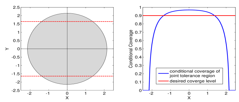
Figure 1: Joint prediction set and pointwise conditional coverage for bivariate independent Gaussian. Left panel: the gray area is the optimal (with smallest Lebesgue measure) prediction set with coverage 0.9, the two red lines are the upper and lower 5% quantiles of the marginal distribution of $Y$. Right panel: the blue curve plots $P(Y\in C(x)|X=x)$ against $x$; the red line is the desired coverage level 0.9.

Figure 1 shows the case of a bivariate independent Gaussian. According to (5), when $X,Y$ are independent standard normals, the level set for any $C^{(\alpha)}$ is a circle centered at the origin as described by the gray area in the left panel of Figure 1. But intuitively since observing $X$ provides no information about $Y$, the best prediction band at level $\alpha$ should be $C(x)=[-z_{\alpha/2},z_{\alpha/2}]$, for all $x$, where $z_{\tau}$ is the $\tau$-th upper quantile of standard normal. This band is the set between two red dashed lines in the left panel of Figure 1 for $\alpha=0.1$.

In prediction, another important notion of coverage is the conditional coverage $P(Y\in C(x)|X=x)$. The pointwise conditional coverage $P(Y\in C(x)|X=x)$ is plotted in the right panel of Figure 1 for the joint prediction set (blue curve). We see that the “optimal” joint prediction set tends to overestimate the set when $x$ is in the high density area and to underestimate for low density $x$. Let us now consider conditional validity in more detail.

2.2 Conditional Validity

Only requiring (2) for prediction bands is not enough. We will refer to (2) as marginal validity or joint validity. This is the type of validity used in Shafer & Vovk (2008). As illustrated in the example above, it may be tempting to insist on a more stringent probability guarantee such as

$$\mathbb{P}(Y_{n+1}\in C_{n}(x)|X_{n+1}=x)\geq 1-\alpha\ \ \ {\rm for\ all\ }P\ {\rm and\ }{\rm almost\ all\ }x,$$ (6)

which we call conditional validity. If the joint distribution of $(X,Y)$ is known, one can define an oracle band as the counterpart of (2) for conditionally valid bands:

$$C_{P}(x)=\Bigl{\{}y:p(y|x)\geq t^{(\alpha)}(x)\Bigr{\}}$$ (7)

where $t^{(\alpha)}(x)$ satisfies

$$\int 1{\hskip-2.5pt}\hbox{I}\left\{p(y|x)\geq t^{(\alpha)}(x)\right\}p(y|x)dy=1-\alpha.$$

We call $C_{P}=\{C_{P}(x):\ x\in\mathbb{R}^{d}\}$ the conditional oracle band. It is easy to prove that $C_{P}$ minimizes $\mu[C(x)]$ for all $x$ among all bands satisfying $\inf_{x}P(Y\in C(x)|X=x)\geq 1-\alpha$. Note that $C_{P}$ depends on $P$ but does not depend on the observed data. For an estimator $\widehat{C}$, asymptotic efficiency requires $\widehat{C}(x)$ be close to $C_{P}(x)$ uniformly over all $x$:

$$\sup_{x}\mu\Bigl{[}\widehat{C}(x)\triangle C_{P}(x)\Bigr{]}\stackrel{{\scriptstyle P}}{{\rightarrow}}0.$$ (8)

However, we will show that there do not exist any prediction bands $\widehat{C}$ that satisfy both (6) and (8). In fact, the following claim, proved in Subsection 8.2, is even stronger.

Let $P_{X}$ denote the marginal distribution of $X$ under $P$. A point $x$ is a non-atom for $P$ if $x$ is in the support of $P_{X}$ and if $P_{X}[B(x,\delta)]\to 0$ as $\delta\to 0$, where $B(x,\delta)$ is the Euclidean ball centered at $x$ with radius $\delta$. Let $N(P)$ denote the set of non-atoms. We show that if $C_{n}$ is conditionally valid then the length of $C_{n}(x)$ is infinite for all $x\in N(P)$.

Lemma 1 (Impossibility of non-trivial finite sample conditional validity).

Suppose that an estimator $C_{n}$ has $1-\alpha$ conditional validity. For any $P$ and any $x_{0}\in N(P)$,

$$\mathbb{P}\Biggl{(}\lim_{\delta\to 0}\operatorname*{ess\,sup}_{||x_{0}-x||\leq\delta}\mu[C_{n}(x)]=\infty\Biggr{)}=1.$$

Thus, non-trivial finite sample conditional validity is impossible for continuous distributions. We shall instead construct prediction bands with an asymptotic version of (6) together with finite sample marginal validity. We say that $\widehat{C}$ is asymptotically conditionally valid if

$$\sup_{x}\Bigl{[}\mathbb{P}(Y_{n+1}\notin C_{n}(x)|X_{n+1}=x)-\alpha\Bigr{]}_{+}\stackrel{{\scriptstyle P}}{{\to}}0$$ (9)

as $n\to\infty$. Here, the supremum is taken over the support of $P_{X}$. We note that if the conditional density $p(y|x)$ is uniformly bounded for all $(x,y)$, then asymptotic conditional validity is a consequence of asymptotic efficiency defined as in (8).

In Section 3 we construct a prediction band that satisfies:

1. finite sample marginal validity,

2. asymptotic conditional validity and

3. asymptotic efficiency.

Our method is based on the notion of local validity, which naturally interpolates between marginal and conditional validity.

Definition 2 (Local validity).

Let $\mathcal{A}=\{A_{j}:j\geq 1\}$ be a partition of ${\rm supp}(P_{X})$ such that each $A_{j}$ has diameter at most $\delta$. A prediction band $C_{n}$ is locally valid with respect to $\cal A$ if

$$\mathbb{P}(Y_{n+1}\in C_{n}(X_{n+1})|X_{n+1}\in A_{j})\geq 1-\alpha,\leavevmode\nobreak\ \leavevmode\nobreak\ {\rm for\ all\ }j\leavevmode\nobreak\ {\rm and\leavevmode\nobreak\ all\leavevmode\nobreak\ }P.$$ (10)

Remark. From the insight of Lemma 1, it is possible to construct finite sample locally valid prediction sets because $X\in A_{j}$ is an event with positive probability and hence repeated observations are available.

Remark. Consider the limiting case of $\delta\rightarrow\infty$, which can be thought as having $A_{1}={\rm supp}(P_{X})$, and local validity becomes marginal validity. On the other hand, in the extremal case $\delta\rightarrow 0$, $A_{j}$ shrinks to a single point $x\in\mathbb{R}^{d}$, and local validity approximates conditional validity. We also note that local validity is stronger than marginal validity but weaker than conditional validity. We state the following proposition whose proof is elementary and omitted.

Proposition 3.

If $C$ is conditionally valid, then it is also locally valid for any partition $\cal A$. If $C$ is locally valid for some partition $\cal A$, then it is also marginally valid.

The relationship between local validity and asymptotic conditional validity is more complicated and is one of the technical contributions of this paper. In Section 3 we construct a specific class of locally valid bands. In Theorem 9 of Section 4 we show that under mild regularity conditions, these bands are also asymptotically conditionally valid. To summarize, if $C$ is locally valid then it is also marginally valid. And under regularity conditions, it can also be asymptotically conditionally valid. See Figure 2.

Figure 2: Relationship between different types of validity.

How can we construct finite sample locally valid prediction bands? A straightforward approach is to apply the method developed in Lei et al. (2011) to $P_{j}\equiv\mathcal{L}(X,Y|X\in A_{j})$, the joint distribution of $(X,Y)$ conditional on the event $X\in A_{j}$. Note that we are mostly interested in the case $\max_{j}{\rm diam}(A_{j})\rightarrow 0$, therefore the marginal density of $X$ within $P_{j}$ becomes increasingly close to uniform. Therefore, the approach can be simplified to finding $C_{j}\in\mathbb{R}^{1}$, such that $P(Y\in C_{j}|X\in A_{j})\geq 1-\alpha$. This approach is detailed in Section 3 and analyzed in Section 4.

3 Methodology

3.1 A Marginally Valid Prediction Band

We start by recalling the construction of joint prediction sets using kernel density together with the idea of conformal prediction, as described in Lei et al. (2011), using the idea of conformal prediction developed in Shafer & Vovk (2008), Vovk et al. (2005) and Vovk et al. (2009). This approach is shown to have finite sample validity as well as asymptotic efficiency under regularity conditions. Suppose we observe

$$Z_{1},\ldots,Z_{n}\sim P$$

and we want a prediction set for $Z_{n+1}$. The idea is to test $H_{0}:Z_{n+1}=z$ for each $z$ and then invert the test. Specifically, for any $z$ let $\widehat{p}_{n}^{z}(\cdot)$ be a density estimator based on the augmented data ${\sf aug}(\mathbf{Z};z)=(Z_{1},\ldots,Z_{n},z)$. Define

$$C_{n}\equiv C_{n}(Z_{1},\ldots,Z_{n})=\left\{z:\ \pi_{n}(z)\geq\alpha\right\}$$

where

$$\pi_{n}(z)=\frac{1}{n+1}\sum_{i=1}^{n+1}1{\hskip-2.5pt}\hbox{I}(\sigma_{i}(z)\leq\sigma_{n+1}(z))$$

is the p-value for the test, $\sigma_{i}(z)=\widehat{p}_{n}^{z}(Z_{i})$ for $i=1,\ldots,n$ and $\sigma_{n+1}(z)=\widehat{p}_{n}^{z}(z)$. The statistic $\sigma_{i}$ is an example of a conformity measure. More generally, a conformity measure $\sigma_{i}(z)=\sigma({\sf aug}(\mathbf{Z},z),Z_{i})$ indicates how well a data point $Z_{i}$ agrees with the augmented data set ${\sf aug}(\mathbf{Z},z)$. In principle $\sigma(\cdot,\cdot)$ can be any function but usually it makes sense to use the fitted residual or likelihood at $Z_{i}$ with respect to a model estimated from ${\sf aug}(\mathbf{Z},z)$.

The intuition for $C_{n}$ is the following. Fix an arbitrary value $z$. To test $H_{0}:Z_{n+1}=z$ we use the heights of the density estimators $\sigma_{i}(z)=\widehat{p}_{n}^{z}(Z_{i})$ as a test-statistic. (Note that $\sigma_{1},\ldots,\sigma_{n+1}$ are functions of ${\sf aug}(\mathbf{Z},z)$.) Under $H_{0}$, the ranks of the $\sigma_{i}$ are uniform, because the joint distribution of $(Z_{1},...,Z_{n},Z_{n+1})$ does not change under permutations. Hence the vector $(\sigma_{1},...,\sigma_{n+1})$ is exchangeable. Therefore, under $H_{0}$, $\pi_{n}(z)$ is uniformly distributed over $[0,1]$ and is a valid p-value for the test. The set $C_{n}$ is obtained by inverting the hypothesis test, that is, $C_{n}$ consists of all values $z$ that are not rejected by the test. It then follows that $\mathbb{P}(Z_{n+1}\in C_{n})\geq 1-\alpha$ for all $P$.

In Lei et al. (2011), the density $\widehat{p}_{n}^{z}$ is obtained from kernel density estimators with bandwidth $h$. Lei et al. (2011) show that $\widehat{C}^{(\alpha)}$ is also efficient meaning that it is close to $C^{(\alpha)}$ with high probability where $C^{(\alpha)}$ is the smallest set with probability content $1-\alpha$ as defined in (5).

Computing $\widehat{C}^{(\alpha)}$ is expensive since we need to find the the p-value $\pi_{n}(z)$ for every $z$. Lei et al. (2011) proposed the following approximation $C_{n}^{+}$ to $C_{n}$—called the sandwich approximation— which avoids the augmentation step altogether but preserves finite sample validity. Let $Z_{(1)},Z_{(2)},\ldots,$ denote the data ordered increasingly by $\widehat{p}(Z_{i})$. Let $j=\lfloor n\alpha\rfloor$ and define

$$C_{n}^{+}=\Biggl{\{}z:\ \widehat{p}(z)\geq\widehat{p}(Z_{(j)})-\frac{K(0)}{nh^{d}}\Biggr{\}}.$$ (11)

Lei et al. (2011) show that $\widehat{C}^{(\alpha)}\subseteq C_{n}^{+}$ and hence $C_{n}^{+}$ also has finite sample validity. Moreover, $C_{n}^{+}$ has the same efficiency properties as $C_{n}$ if $h$ is chosen appropriately. This result, known as the “Sandwich Lemma”, provides a simple characterization of the conformal prediction set $\widehat{C}^{(\alpha)}$ in terms of the plug-in density level set. In this paper, a specific version of the Sandwich Lemma for the conditional density is stated in Lemma 8. Thus, using the sandwich approximation we get a fast method for constructing a valid band, based on slicing the joint density.

Now let $Z=(X,Y)$. The $x$-slices of the joint region for $Z$ define a marginally valid band. Specifically, let $K_{x}$ and $K_{y}$ be two kernel functions in $\mathbb{R}^{d}$ and $\mathbb{R}^{1}$, respectively. Consider the kernel density estimator: For any $(u,v)\in\mathbb{R}^{d}\times\mathbb{R}^{1}$:

$$\widehat{p}_{n;X,Y}(u,v)=\frac{1}{n}\sum_{i=1}^{n}\frac{1}{h_{n}^{d+1}}K_{x}\left(\frac{u-X_{i}}{h_{n}}\right)K_{y}\left(\frac{v-Y_{i}}{h_{n}}\right).$$ (12)

For any $(x,y)\in\mathbb{R}^{d}\times\mathbb{R}^{1}$, let $({\bf X,Y})=(X_{1},Y_{1},\ldots,X_{n},Y_{n})$ be the data set and ${\sf aug}({\bf X},{\bf Y};(x,y))$ be the augmented data with $X_{n+1}=x$ and $Y_{n+1}=y$. Define $\widehat{p}^{(x,y)}_{n;X,Y}$ be the kernel density estimator from the augmented data:

$$\widehat{p}_{n;X,Y}^{(x,y)}(u,v)=\frac{n}{n+1}\widehat{p}_{n;X,Y}(u,v)+\frac{1}{(n+1)h_{n}^{d+1}}K_{x}\left(\frac{u-x}{h_{n}}\right)K_{y}\left(\frac{v-y}{h_{n}}\right)\,.$$ (13)

Define the conformity measure

$$\sigma_{i}(x,y):=\widehat{p}_{n;X,Y}^{(x,y)}(X_{i},Y_{i}).$$ (14)

and p-value

$$\pi_{i}=\frac{1}{n+1}\sum_{j=1}^{n+1}1{\hskip-2.5pt}\hbox{I}(\sigma_{j}(x,y)\leq\sigma_{i}(x,y))\,,\quad{\rm for}\quad 1\leq i\leq n+1.$$ (15)

Let $\widetilde{\alpha}=\lfloor(n+1)\alpha\rfloor/(n+1).$ Since $(X_{i},Y_{i})_{i=1}^{n+1}$ are iid, by exchangeability, we have, for all $i$,

$$\mathbb{P}(\pi_{i}\geq\widetilde{\alpha})\geq 1-\alpha.$$ (16)

Define

$$\widehat{C}^{(\alpha)}(x)=\left\{y:\pi_{n+1}(x,y)\geq\widetilde{\alpha}\right\},$$

where $\pi_{n+1}\equiv\pi_{n+1}\left[{\sf aug}({\bf X,Y};(x,y))\right]$. From (16) we have:

Lemma 4.

$\widehat{C}^{(\alpha)}(x)$ is finite sample marginally valid:

$$\mathbb{P}\left[Y_{n+1}\in\widehat{C}^{(\alpha)}(X_{n+1})\right]\geq 1-\alpha\ \ \ {\rm for\ all\ }P.$$

Now we use the sandwich approximation to the joint conformal region for $(X,Y)$. The resulting band $C_{n}^{+}(x)$ is obtained by fixing $X=x$ and taking slices of the joint region and is then a marginally valid band. See Algorithm 1.

Algorithm 1. Sandwich Slicer Algorithm 1. Let $\widehat{p}(x,y)$ be the joint density estimator. 2. Let $Z_{i}=(X_{i},Y_{i})$ and let $Z_{(1)},Z_{(2)},\ldots,$ denote the sample ordered increasingly by $\widehat{p}(X_{i},Y_{i})$. 3. Let $j=\lfloor n\alpha\rfloor$ and define $$C_{n}^{+}(x)=\left\{y:\ \widehat{p}(x,y)\geq\widehat{p}(X_{(j)},Y_{(j)})-\frac{K_{x}(0)K_{y}(0)}{nh^{d+1}}\right\}.$$ (17)

To summarize: the band given in Algorithm 1 is marginally valid. But it is not efficient nor does it satisfy asymptotic conditional validity. This leads to the subject of the next section.

3.2 Locally Valid Bands

Now we extend the idea of conformal prediction to construct prediction bands with local validity. These bands will also be asymptotically efficient and have asymptotic conditional validity. For simplicity of presentation, we assume that ${\rm supp}(P_{X})=[0,1]^{d}$ where ${\rm supp}(P_{X})$ denotes the support of $P_{X}$ and we consider partitions $\mathcal{A}=\{A_{k},k\geq 1\}$ in the form of cubes with sides of length $w_{n}$. Let $n_{k}=\sum_{i=1}^{n}\mathbf{1}(X_{i}\in A_{k})$ be the histogram count.

Given a kernel function $K(\cdot):\mathbb{R}^{1}\mapsto\mathbb{R}^{1}$ and another bandwidth $h_{n}$, consider the estimated local marginal density of $Y$:

$$\widehat{p}(y|A_{k})=\frac{1}{n_{k}h_{n}}\sum_{i=1}^{n}1{\hskip-2.5pt}\hbox{I}(X_{i}\in A_{k})K\left(\frac{Y_{i}-y}{h_{n}}\right).$$

The corresponding augmented estimate is, for any $(x,y)\in A_{k}\times\mathbb{R}^{1}$,

$$\widehat{p}^{(x,y)}(v|A_{k})=\frac{n_{k}}{n_{k}+1}\widehat{p}(v|A_{k})+\frac{1}{(n_{k}+1)h_{n}}K\left(\frac{v-y}{h_{n}}\right).$$ (18)

For any $(x,y)\in A_{k}\times\mathbb{R}^{1}$, consider the following local conformity rank

$$\pi_{n,k}(x,y)=\frac{1}{n_{k}+1}\sum_{i=1}^{n+1}1{\hskip-2.5pt}\hbox{I}(X_{i}\in A_{k})1{\hskip-2.5pt}\hbox{I}\left[\widehat{p}^{(x,y)}(Y_{i}|A_{k})\leq\widehat{p}^{(x,y)}(Y_{n+1}|A_{k})\right]\,,$$ (19)

which can be interpreted as the local conditional density rank. It is easy to check that the $\pi_{n,k}(x,y)$ has a sub-uniform distribution if $(X_{n+1},Y_{n+1})=(x,y)$ is another independent sample from $P$. Therefore, the band

$$\widehat{C}(x)=\{\pi_{n,k}(x,y)\geq\alpha\}$$ (20)

for $x\in A_{k}$ has finite sample local validity.

Proposition 5.

For $x\in A_{k}$, let $\widehat{C}(x)=\{y:\pi_{n,k}(x,y)\geq\alpha\}$, where $\pi_{n,k}(x,y)$ is defined as in (19), then $\widehat{C}(x)$ is finite sample locally valid and hence finite sample marginally valid.

Proof.

Fix $k$, let $\{i_{1},...,i_{n_{k}}\}=\{i:1\leq i\leq n,\leavevmode\nobreak\ X_{i}\in A_{k}\}$. Let $(X_{n+1},Y_{n+1})\sim P$ be another independent sample. Define $i_{n_{k}+1}=n+1$ and $\sigma_{i_{\ell}}=\widehat{p}^{(x,y)}(Y_{i_{\ell}}|A_{k})$ for all $1\leq\ell\leq n_{k}+1$. Then conditioning on the event $X_{n+1}\in A_{k}$ and $(i_{1},...,i_{n_{k}})$, the sequence $(\sigma_{i_{1}},...,\sigma_{i_{n_{k}}},\sigma_{i_{n_{k}+1}})$ is exchangeable. ∎

We call $\widehat{C}$ the Conformal Optimized Prediction Set (COPS) estimator, where the word “optimized” stands for the effort of minimizing the average interval length $\mathbb{E}_{X}\widehat{C}(X)$.

We give a fast approximation algorithm that is analogous to Algorithm 1. The resulting approximation also satisfies finite sample local validity as well as asymptotic efficiency as shown in Section 4. See Algorithm 2.

Algorithm 2: Local Sandwich Slicer Algorithm 1. Divide ${\cal X}$ into bins $A_{1},\ldots,A_{m}$. 2. Apply Algorithm 1 separately on all $Y_{i}$’s within each $A_{k}$. 3. Output $C_{n}^{+}(x)$: the resulting set of $A_{k}$ for all $x\in A_{k}$.

Remark 6.

In the approach described above, the local conformity measure is $\widehat{p}^{(x,y)}(v|A_{k})$. In principle one can use any conformity measure that does not need to depend on the partition $A_{k}$, as long as the symmetry condition is satisfied. For example, one can use either the estimated joint density $\widehat{p}^{(x,y)}(u,v)$ or the estimated conditional density $\widehat{p}^{(x,y)}(v|u)$. We note that when ${\sf diam}(A_{k})$ is small, these choices of conformity measure are close to each other since $p_{X}(x)$ and $p(\cdot|x)$ change very little when $x$ varies inside $A_{k}$.

Remark 7.

Although one can choose any conformity measure, in order to have local validity the ranking must be based on a local subset of the sample. When $A_{k}$ is small and the distribution is smooth enough, the local sample $(X_{i_{\ell}}:1\leq\ell\leq n_{k})$ approximates independent observations from $p(\cdot|X=x)$ for $x\in A_{k}$, which can be used to approximate the conditional oracle $C_{P}(x)$.

4 Asymptotic Properties

In this section we investigate the asymptotic efficiency of the locally valid prediction band given in (20). The efficiency argument is similar for other choices of conformity measures, such as joint density or conditional density. Again, we focus on cases where ${\rm supp}(P_{X})=[0,1]^{d}$ and $\mathcal{A}$ is a cubic histogram with width $w_{n}$. The conformity measure is $\widehat{p}^{(x,y)}(Y_{i}|A_{k})$ for $x\in A_{k}$, where $\widehat{p}^{(x,y)}(v|A_{k})$ is defined as in equation (18) with kernel bandwidth $h_{n}$.

4.1 Notation

In the subsequent arguments, $p_{X}(\cdot)$ denotes the marginal density of $X$, $p(y|x)$ the conditional density of $Y$ given $X=x$, and $p(y|A_{k})$ the conditional density of $Y$ given $X\in A_{k}$. The kernel estimator of $p(y|A_{k})$ is denoted by $\widehat{p}(\cdot|A_{k})$ and $\widehat{P}(\cdot|A_{k})$ is the empirical distribution of $(Y|X\in A_{k})$.

The upper and lower level sets of conditional density $p(y|x)$ are denoted by $L_{x}(t)\equiv\{y:p(y|x)\geq t\}$ and $L_{x}^{\ell}(t)\equiv\{y:p(y|x)\leq t\}$, respectively; $\widehat{L}_{k}(t)$, $\widehat{L}_{k}^{\ell}(t)$ are the counterparts of $L_{x}(t)$ and $L_{x}^{\ell}(t)$, defined for $\widehat{p}(\cdot|A_{k})$. As in the definition of conditional oracle, $t_{x}^{(\alpha)}$ is solution to the equation $P_{x}(L_{x}(t))=1-\alpha$. Its existence and uniqueness is guaranteed if the contour $\{y:p(y|x)=t\}$ has zero measure for all $t>0$. Finally we let $G_{x}(t)=P_{x}(L_{x}^{\ell}(t))$.

4.2 The Sandwich Lemma

Heuristically, $\widehat{p}(y|A_{k})\approx p(y|x)$ for $x\in A_{k}$ when ${\rm diam}(A_{k})$ is small and $p(y|x)$ varies smoothly in $x$. As a result, the estimated densities $\widehat{p}^{(x,y)}(Y_{i}|A_{k})$ can be viewed as roughly a sample from $p(Y|x)$, and hence $\widehat{C}(x)$ approximates the conditional oracle $C_{P}(x)$. First we show that $\widehat{C}(x)$ can be approximated by two plug-in conditional density level sets (Lemma 8). For a fixed $A_{k}\in\mathcal{A}$, conditioning on $(i_{1},...,i_{n_{k}})$, let $(X_{(k,\alpha)},Y_{(k,\alpha)})$ be the element of $\{(X_{i_{1}},Y_{i_{1}}),$ $...,(X_{i_{n_{k}}},Y_{i_{n_{k}}})\}$ such that $\widehat{p}(Y_{(k,\alpha)}|A_{k})$ ranks $\lfloor n_{k}\alpha\rfloor$ in ascending order among all $\widehat{p}(Y_{i_{j}}|A_{k})$, $1\leq j\leq n_{k}$.

Lemma 8 (The Sandwich Lemma (Lei et al., 2011)).

For any fixed $\alpha\in(0,1)$, if $\widehat{C}(x)$ is defined in (20) and $||K||_{\infty}=K(0)$, then $\widehat{C}(x)$ is “sandwiched” by two plug-in conditional density level sets:

$$\widehat{L}\left(\widehat{p}\left(X_{(k,\alpha)},Y_{(k,\alpha)}|A_{k}\right)\right)\subseteq\widehat{C}(x)\subseteq\widehat{L}\left(\widehat{p}(X_{(k,\alpha)},Y_{(k,\alpha)}|A_{k})-(n_{k}h_{n})^{-1}\psi_{K}\right),$$ (21)

where $\psi_{K}=\sup_{x,x^{\prime}}|K(x)-K(x^{\prime})|$.

The Sandwich Lemma provides simple and accurate characterization of $\widehat{C}(x)$ in terms of plug-in conditional density level sets, which are much easier to estimate. The asymptotic properties of $\widehat{C}(x)$ can be obtained by those of the sandwiching sets.

4.3 Rates of convergence

To show the asymptotic efficiency of $\widehat{C}(x)$, it suffices to show efficiency for both sandwiching sets in Lemma 8. We need regularity conditions to quantify and control the approximations $p(y|x)\approx p(y|A_{k})$, $\widehat{p}(y|A_{k})\approx p(y|A_{k})$, and $\widehat{L}_{k}(t)\approx L_{x}(t)$.

The following assumption puts boundedness and smoothness conditions on the marginal density $p_{X}$, conditional density $p(y|x)$, and its derivatives.

Assumption A1 (regularity of marginal and conditional densities)

1. The marginal density of $X$ satisfies $0<p_{0}\leq p_{X}(x)\leq p_{1}<\infty$ for all $x$.

2. For all $x$, $p(\cdot|x)$ is Hölder class $\mathcal{P}(\beta,L)$. Correspondingly, the kernel $K$ is a valid kernel of order $\beta$.

3. For any $0\leq s\leq\lfloor\beta\rfloor$, $p^{(s)}(y|x)$ is continuous and uniformly bounded by $L$ for all $x,y$.

4. The conditional density is Lipschitz in $x$: $||p(\cdot|x)-p(\cdot|x^{\prime})||_{\infty}\leq L||x-x^{\prime}||$.

The Hölder class of smooth functions and valid kernels are common concepts in nonparametric density estimation. We give their definitions in Appendix 8.1. Assumptions A1(b) and A1(c) implies that $p(\cdot|A_{k})$ is also in a Hölder class and can be estimated well by kernel estimators. A2(d) enables us to approximate $p(\cdot|x)$ by $p(\cdot|A_{k})$ for all $x\in A_{k}$.

The next assumption gives sufficient regularity condition on the level sets $L_{x}(t)$.

Assumption A2 (regularity of conditional density level set)

1. There exist positive constants $\epsilon_{0}$, $\gamma$, $c_{1}$, $c_{2}$, such that

   $$c_{1}(t_{2}-t_{1})^{\gamma}\leq G_{x}(t_{2})-G_{x}(t_{1})\leq c_{2}(t_{2}-t_{1})^{\gamma},$$

   for all $t_{x}^{(\alpha)}-\epsilon_{0}\leq t_{1}\leq t_{2}\leq t_{x}^{(\alpha)}+\epsilon_{0}$.

2. There exist positive constants $t_{0}$ and $C$, such that $0<t_{0}<\inf_{x}t_{x}^{(\alpha)}$ and $\mu(L_{x}(t_{0}))<C$ for all $x$.

Assumption A2(a) is related to the notion of “$\gamma$-exponent” condition introduced by Polonik (1995) and widely used in the density level set literature (Tsybakov, 1997; Rigollet & Vert, 2009). It ensures that the conditional density function $p(\cdot|x)$ is neither too flat nor too steep near the contour at level $t_{x}^{(\alpha)}$, so that the cut-off value $t_{x}^{(\alpha)}$ and the conditional density level set $C_{P}(x)$ can be approximated from a finite sample. As mentioned in Audibert & Tsybakov (2007), if Assumption A1(b) also holds, the oracle band $C_{P}(x)$ is non-empty only if $\gamma(\beta\wedge 1)\leq 1$, which holds for the most common case $\gamma=1$. Part (b) simply simply puts some constraints on the optimal levels as well as the size of the level sets.

The following critical rate will be used repeatedly in our analysis.

$$r_{n}=\left(\frac{\log n}{n}\right)^{\frac{\beta}{\beta(d+2)+1}}.$$ (22)

The rate may appear to be non-standard. This is because we are assuming difference amounts of smoothness on $y$ and $x$. This seems to be necessary to achieve both marginal and local validity. We do not know of any procedure that uses a smoother construction and still retains finite sample validity. The next theorem gives the convergence rate on the asymptotic efficiency of the locally valid prediction band constructed in Subsection 3.2.

Theorem 9.

Let $\widehat{C}$ be the prediction band given by the local conformity procedure as described in (20). Choose $w_{n}\asymp r_{n}$, $h_{n}\asymp r_{n}^{1/\beta}$. Under Assumptions A1-A2, for any $\lambda>0$, there exists constant $A_{\lambda}$, such that

$$\mathbb{P}\left(\sup_{x\in\mathcal{X}}\mu\left(\widehat{C}(x)\triangle C_{\rm P}(x)\right)\geq A_{\lambda}r_{n}^{\gamma_{1}}\right)=O(n^{-\lambda}),$$

where $\gamma_{1}=\min(1,\gamma)$.

Thus, in the common case $\gamma=1$, the rate is $r_{n}$. The following lemma follows easily from the previous result.

Lemma 10.

Under assumptions A1 and A2, the local band is asymptotically conditionally valid.

Remark 11.

It follows from the proof that the output of Algorithm 2 also satisfies the same asymptotic efficiency and conditional validity results.

4.4 Minimax Bound

The next theorem says that in the most common case $\gamma=1$, the rate given in Theorem 9 is indeed minimax rate optimal. We define the minimax risk by

$$\inf_{\widehat{C}\in{\cal C}_{n,\alpha}}\sup_{P\in\mathcal{P}(\beta,L)}\mathbb{E}_{P}\mu\left[\widehat{C}(x)\triangle C(x)\right]$$ (23)

where ${\cal C}_{n,\alpha}$ is the set of all valid prediction sets, and $\mathcal{P}(\beta,L)$ is the class of distributions satisfying A1 and A2 with $\gamma=1$. We can obtain a lower bound on the minimax risk by taking the infimum over all set estimators $\widehat{C}$, as in the following result.

Theorem 12 (Lower bound on estimation error).

Let $\mathcal{P}(\beta,L)$ be the class of distributions on $[0,1]^{d}\times\mathbb{R}^{1}$ such that for each $P\in\mathcal{P}(\beta,L)$, $P_{X}$ is uniform on $[0,1]^{d}$, and satisfies Assumptions A1-A2 with $\gamma=1$. Fix an $\alpha\in(0,1)$, there exist constant $c=c(\alpha,\beta,L,d)>0$ such that

$$\inf_{\widehat{C}}\sup_{P\in\mathcal{P}(\beta,L)}\mathbb{E}_{P}\mu\left[\widehat{C}(x)\triangle C(x)\right]\geq cr_{n}.$$

Hence, our procedure achieves the same rate as the lower bound and so is minimax rate optimal over the class $\mathcal{P}(\beta,L)$. The proof of Theorem 12 is in Section 8.4 and uses a somewhat non-standard construction.

5 Tuning Parameter Selection

In the band given by (20), there are two bandwidths to choose: $w_{n}$ and $h_{n}$. Note that since each bin $A_{k}$ can use a different $h_{n}$ to estimate the local marginal density $\widehat{p}(\cdot|A_{k})$, we can consider $h_{n,k}$, allowing a different kernel bandwidth for each bin.

Since all bandwidths give local validity, one can choose the combination of $(w_{n},h_{n,k})$ such that the resulting conformal set has smallest Lesbesgue measure. Such a two-stage procedure of selecting $w_{n}$ and $h_{n,k}$ from discrete candidate sets $\mathcal{W}=\{w^{1},...,w^{m}\}$ and $\mathcal{H}=\{h^{1},...,h^{\ell}\}$ is detailed in Algorithm 3. To preserve finite sample marginal validity with data-driven bandwidths, we split the sample into two equal-sized subsamples, and apply the tuning algorithm on one subsample and use the output bandwidth on the other subsample to obtain the prediction band.

Algorithm 3: Bandwidth Tuning for COPS Input: Data $\mathcal{Z}$, level $\alpha$, candidate sets $\mathcal{W}$, $\mathcal{H}$. 1. Split data set into two equal sized subsamples, $\mathcal{Z}_{1}$, $\mathcal{Z}_{2}$. 2. For each $w\in\mathcal{W}$ (a) Construct partition $\mathcal{A}^{w}$. (b) For each $k$ and $h$ construct local conformal prediction set $\widehat{C}_{h,k}^{1}$, each at level $1-\alpha$, using data $\mathcal{Z}_{1}$. (c) Let $h^{*}_{w,k}=\arg\min_{h\in\mathcal{H}}\mu\big{(}\widehat{C}_{h,k}^{1}\big{)}$, for all $k$. (d) Let $Q(w)=\frac{1}{n}\sum_{k}n_{k}\mu\big{(}\widehat{C}^{1}_{h^{*}_{w,k},k}\big{)}$. 3. Choose $\widehat{w}=\arg\min Q(w)$; $\widehat{h}_{\widehat{w},k}=h^{*}_{\widehat{w},k}$. 4. Construct partition $\mathcal{A}^{\widehat{w}}$. For $x\in A_{k}$, output prediction band $\widehat{C}(x)=\widehat{C}_{\widehat{h}_{\widehat{w},k},k}^{2}$, where $\widehat{C}_{h,k}^{2}$ is the local conformal prediction set estimated from data $\mathcal{Z}_{2}$ in local set $A_{k}$.

Following Remark 6, one can use different conformity measures to construct $\widehat{C}$. In principle, the above sample splitting procedure works for any conformity measures.

It is straightforward to show that the band $\widehat{C}$ constructed as above using data-driven tuning parameters is locally valid and marginally valid, because the bandwidth $(w,h)$ used is independent of the training data $\mathcal{Z}_{2}$. From the construction of $\widehat{C}$, it will have small excess risk if the conformal prediction set is stable under random sampling. Then asymptotic efficiency follows if one can relate the excess risk to the symmetric difference risk. A rigorous argument is beyond the scope of this paper and will be pursued in a separate paper.

6 Data Examples

In this section we apply our method to some examples.

6.1 A Synthetic Example

The procedure is illustrated by the following example in which $d=1$, and

$$\begin{array}[]{rl}X\sim&{\sf Unif}[-1.5,1.5]\,,\\ (Y|X=x)\sim&0.5N\left[f(x)-g(x),\sigma^{2}(x)\right]+0.5N\left[f(x)+g(x),\sigma^{2}(x)\right]\,,\end{array}$$ (24)

where

$$f(x)= (x-1)^{2}(x+1),$$

$$g(x)= 2\sqrt{x+0.5}\times 1{\hskip-2.5pt}\hbox{I}(x\geq-0.5),$$

$$\sigma^{2}(x)= 1/4+|x|.$$

For $x\leq-0.5$, $(Y|X=x)$ is a Gaussian centered at $f(x)$ with varying variance $\sigma^{2}(x)$. For $x\geq-0.5$, $(Y|X=x)$ is a two-component Gaussian mixture, and for large values of $x$, the two components have little overlap.

Figure 3: Conditional and marginal prediction bands. The bottom left panel shows the relationship between bandwidth and Lebesgue measure of the prediction band. The bottom right panel shows the conditional coverage of the estimated set $\widehat{C}(x)$ as a function of $x$.

The performance of prediction bands using local conformity is plotted and compared with the marginal valid band in Figure 3, with $n=1000$, $\alpha=0.1$. The conformity measure used here is $\widehat{p}^{(x,y)}(Y_{i}|X_{i})$. The locally valid prediction band is constructed by partitioning the support of $P_{X}$ into 10 equal sized bins, whereas the marginally valid band is constructed by a global ranking with the same conformity measure. We see that although the locally valid band has larger Lebesgue measure, it gives the desired coverage for all values $x$. The marginally valid band over covers for smaller values of $x$, and under covers for larger values of $x$. We also plot the effect of bandwidth on the size of prediction set (lower left panel of Figure 3).

6.2 Car Data

Next we consider an example on car mileage. The original data contains features for about 400 cars. For each car, the data consist of miles per gallon, horse power, engine displacement, size, acceleration, number of cylinders, model year, origin of manufacture. These data have been used in statistics text books (for example, DeGroot & Schervish (2012), Chapter 11) to illustrate the art of linear regression analysis. Here we reproduce the linear model built in Example 11.3.2 of DeGroot & Schervish (2012), where we want to predict the miles per gallon by the horse power. Clearly, the relationship between miles per gallon and horse power is far from linear (Figure 4) so some transformation must be applied prior to linear model fitting. It makes sense to assume, both from intuition and data plots, that the inverse of miles per gallon, namely, gallons per mile, has roughly a linear dependence on the horse power.

In the right panel of Figure 4 we plot the level 0.9 prediction band obtained from the linear regression prediction band. The overall coverage is reasonably close to the nominal level. However, due to the non-uniform noise level, the band is too wide for small values of horse power and too narrow for large values. In the left panel, we plot the nonparametric conformal prediction band using conformity measure $\widehat{p}_{h}^{y}(Y_{i}|X_{i})$ to enhance smoothness of the estimated band. Such a band is asymptotically close to the one given in (20). The bandwidths are $h_{x}=14$ and $h_{y}=1.4$. The partition $\mathcal{A}$ is constructed by partitioning the range of horse power into several intervals to ensure each set $A_{k}$ contains roughly same number of sample points. Here the tuning parameter is the number of partitions and is set to 8.

The advantage of our method is clear. First, it automatically outputs good prediction bands without involving choosing the variable transformation. The tuning parameters can be chosen in either an automated procedure as described in Algorithm 3, or by conventional choices (kernel bandwidth selectors). Second, the conformal prediction band is truly distribution free, with valid coverage for all distribution and all sample sizes.

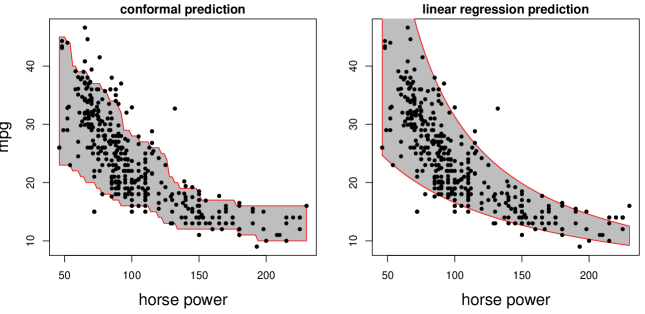
Figure 4: Level $.9$ prediction bands using local conformal prediction (left) and linear regression with variable transformation (right).

7 Final Remarks

We have constructed nonparametric prediction bands with finite sample, distribution free validity. With regularity assumptions, the band is efficient in the sense of achieving the minimax bound. The tuning parameters are completely data-driven. We believe this is the first prediction band with these properties.

An important open question is to establish a rigorous result on the asymptotic efficiency for the data-driven bandwidth. A sketch of such an argument can be given by combining two facts. First, the empirical average excess loss $n^{-1}\sum_{k}n_{k}\mu(\widehat{C}_{h,k})$ is a good approximation to the excess risk $\mathbb{E}\left[\int\mu(\widehat{C}_{h,k}(x))P_{X}(dx)\right]$ for all $w$ and $h$. This problem is technically similar to those considered by Rinaldo et al. (2010) in the study of stability of plug-in density level sets and prediction sets. Second, one can show that the excess risk provides an upper bound of the symmetric difference risk $\mathbb{E}(\widehat{C}\triangle C_{P})$, as given in Lei et al. (2011) (see also Scott & Nowak (2006)).

The bands are not suitable for high-dimensional regression problems. In current work, we are developing methods for constructing prediction bands that exploit sparsity assumptions. These will yield valid prediction and variable selection simultaneously.

8 Appendix

In the appendix, we give supplementary technical details.

8.1 Technical Definitions

Now we give formal definitions of some technical terms used in the asymptotic analysis, including Hölder class of functions and valid kernel functions of order $\beta$. These definitions can be found in standard nonparametric inference text books such as (Tsybakov, 2009, Section 1.2).

Definition 13 (Hölder Class).

Given $L>0$, $\beta>0$. Let $\ell=\lfloor\beta\rfloor$. The Hölder class $\Sigma(\beta,L)$ is the family of functions $f:\mathbb{R}^{1}\mapsto\mathbb{R}^{1}$ whose derivative $f^{(\ell)}$ satisfies

$$|f^{(\ell)}(x)-f^{(\ell)}(x^{\prime})|\leq L|x-x^{\prime}|^{\beta-\ell},\leavevmode\nobreak\ \forall\leavevmode\nobreak\ x,x^{\prime}.$$

Remark: If $f\in\Sigma(\beta,L)$, then $f$ can be uniformly approximated by its local polynomials of order $\ell$. Define

$$f_{x_{0}}^{(\ell)}(x)=f(x_{0})+f^{\prime}(x_{0})(x-x_{0})+....+\frac{f^{(\ell)}(x_{0})}{\ell!}(x-x_{0})^{\ell}.$$

Then

$$|f(x)-f_{x_{0}}^{(\ell)}(x)|\leq\frac{L}{\ell!}|x-x_{0}|^{\beta}.$$

Definition 14 (Valid Kernels of Order $\beta$).

Let $\beta>0$ and $\ell=\lfloor\beta\rfloor$. Say that $K:\mathbb{R}^{1}\mapsto\mathbb{R}^{1}$ is a valid kernel of order $\beta$ if the functions $u\mapsto u^{j}K(u)$, $j=1,...,\ell$, are integrable and satisfy

$$\int K(u)du=1,\leavevmode\nobreak\ \leavevmode\nobreak\ \int u^{j}K(u)du=0,\leavevmode\nobreak\ j=1,...,\ell.$$

Remark: The relationship between a Hölder class $\Sigma(\beta,L)$ and a valid kernel $K$ of order $\beta$ is that for any $p\in\Sigma(\beta,L)$, and $h=o(1)$, $||p-p\star K_{h}||_{\infty}\leq\frac{L}{\ell!}h^{\beta}$, where $\star$ is the convolution operator and $K_{h}(x)=h^{-1}K(x/h)$.

8.2 Proof of Lemma 1

Proof of Lemma 1.

For simplicity we prove the case where $d=1$. Let

$${\sf TV}(P,Q)=\sup_{A}|P(A)-Q(A)|$$

denote the total variation distance between $P$ and $Q$. Given any $\epsilon>0$ define

$$\epsilon_{n}=2[1-(1-\epsilon^{2}/8)^{1/n}].$$

From Lemma A.1 of Donoho (1988), if ${\sf TV}(P,Q)\leq\epsilon_{n}$ then ${\sf TV}(P^{n},Q^{n})\leq\epsilon$.

Fix $\epsilon>0$. Let $x_{0}$ be a non-atom and choose $\delta$ be such that $0<P_{X}\left[B(x_{0},\delta)\right]<\epsilon_{n}$ where $\epsilon_{n}=2[1-(1-\epsilon^{2}/8)^{1/n}]$. It follows that ${\sf TV}(P^{n},Q^{n})\leq\epsilon$.

Fix $B>0$ and let $B_{0}=B/(2(1-\alpha))$. Define another distribution $Q$ by

$$Q(A)=P(A\cap S^{c})+U(A\cap S)$$

where

$$S=\Bigl{\{}(x,y):\ x\in B(x_{0},\delta),\ y\in\mathbb{R}\Bigr{\}}$$

and $U$ has total mass $P(S)$ and is uniform on $\{(x,y):\ x\in B(x_{0},\delta),\ |y|<B_{0}\}$. Note that $P(S)>0$, $Q(S)>0$ and ${\sf TV}(P,Q)\leq\epsilon_{n}$. It follows that ${\sf TV}(P^{n},Q^{n})\leq\epsilon$.

Note that, for all $x\in B(x_{0},\delta)$, $\int_{C(x)}q(y|x)dy\geq 1-\alpha$ implies that $\mu[C(x)]\geq 2(1-\alpha)B_{0}=B$. Hence,

$$Q^{n}\Biggl{(}\operatorname*{ess\,sup}_{x\in B(x_{0},\delta)}\mu[C(x)]\geq B\Biggr{)}=1.$$

Thus,

$$P^{n}\Biggl{(}\operatorname*{ess\,sup}_{x\in B(x_{0},\delta)}\mu[C(x)]\geq B\Biggr{)}\geq Q^{n}\Biggl{(}\operatorname*{ess\,sup}_{x\in B(x_{0},\delta)}\mu[C(x)]\geq B\Biggr{)}-\epsilon=1-\epsilon.$$

Since $\epsilon$ and $B$ are arbitrary, the result follows. ∎

8.3 Proofs of asymptotic efficiency

Lemma 15.

Given $\lambda>0$, under condition A2 and A4, there exists numerical constant $\xi_{\lambda}$ such that,

$$\mathbb{P}\left(\sup_{k}||\widehat{p}(\cdot|A_{k})-p(\cdot|A_{k})||_{\infty}\geq\xi_{\lambda}r_{n}\right)=O(n^{-\lambda}).$$

Proof.

for any fixed $k$, $Y_{i_{1}},...,Y_{i_{n_{k}}}$ is a random sample from $P(y|A_{k})$ conditioning on $n_{k}$.

Let $\bar{p}(y|A_{k})$ be the convolution density $p(\cdot|A_{k})\star K_{h_{n}}(\cdot)$, then using a result from Giné & Guillou (2002), there exists numerical constants $C_{1}$, $C_{2}$ and $\xi_{0}$ such that for all $\xi\geq\xi_{0}$,

$$\mathbb{P}\left(||\widehat{p}(\cdot|A_{k})-\bar{p}(\cdot|A_{k})||_{\infty}\geq\xi\sqrt{\log n_{k}/(n_{k}h_{n})}\right)\leq C_{1}h_{n}^{C_{2}\xi^{2}}.$$ (25)

On the other hand, by Hölder condition of $p(y|x)$ and hence on $p(\cdot|A_{k})$, we have:

$$||\bar{p}(\cdot|A_{k})-p(\cdot|A_{k})||_{\infty}\leq Lh_{n}^{\beta}.$$

Put together with union bound on all $A_{k}\in\mathcal{A}_{n}$

$$\mathbb{P}\left(\exists k:\leavevmode\nobreak\ ||\widehat{p}(\cdot|A_{k})-p(\cdot|A_{k})||_{\infty}\geq\xi\sqrt{\log n_{k}/(n_{k}h_{n})}+Lh_{n}^{\beta}\right)\leq C_{1}h_{n}^{C_{2}\xi^{2}}w_{n}^{-d}.$$

Consider event $E_{0}$:

$$E_{0}=\{b_{1}nw_{n}^{d}/2\leq n_{k}\leq 3b_{2}nw_{n}^{d}/2\},$$

where the constants $b_{1}$ and $b_{2}$ is defined as in Assumption A1(a). By Lemma 20 we have

$$\mathbb{P}(E_{0}^{c})\leq C_{3}w_{n}^{-d}\exp(-C_{4}nw_{n}^{d}),$$

with constants $C_{3}$, $C_{4}$ defined in lemma 20.

On $E_{0}$ and for $n$ large enough we have

$$\sqrt{\frac{\log n_{k}}{n_{k}h_{n}}}\leq 2\sqrt{\frac{2\beta+1}{c_{1}\left[\beta(d+2)+1\right]}}\sqrt{\frac{\log n}{nw_{n}^{d}h_{n}}}.$$

Note that under Assumption A4, $\sqrt{\frac{\log n}{nw_{n}^{d}h_{n}}}=h_{n}^{\beta}=r_{n}$.

Let

$$\xi_{\lambda}=2\sqrt{\frac{2\beta+1}{c_{1}\left[\beta(d+2)+1\right]}}\left(\sqrt{\frac{\lambda(\beta(d+2)+1)+\beta d}{C_{2}}}\bigvee\xi_{0}\right)+L,$$

where the constant $c_{1}$ is defined in Assumption A1(a), $C_{2}$ defined in equation (25), and $L$ defined in A2(a).

Then we have

$$\mathbb{P}\left(\sup_{k}||\widehat{p}(\cdot|A_{k})-p(\cdot|A_{k})||_{\infty}\leq\xi_{\lambda}r_{n}\right)$$

$$\geq \mathbb{P}\left(\sup_{k}||\widehat{p}(\cdot|A_{k})-p(\cdot|A_{k})||_{\infty}\leq(\xi_{\lambda}-L)\sqrt{\frac{\log n}{nw_{n}^{d}h_{n}}}+Lh_{n}^{\beta},\leavevmode\nobreak\ E_{0}\right)$$

$$\geq \mathbb{P}\left(\sup_{k}||\widehat{p}(\cdot|A_{k})-p(\cdot|A_{k})||_{\infty}\leq\frac{\xi_{\lambda}-L}{2\sqrt{\frac{2\beta+1}{c_{1}\left[\beta(d+2)+1\right]}}}\sqrt{\frac{\log n_{k}}{n_{k}h_{n}}}+Lh_{n}^{\beta},\leavevmode\nobreak\ E_{0}\right)$$

$$\geq 1-\mathbb{P}\left(\exists k:||\widehat{p}(\cdot|A_{k})-p(\cdot|A_{k})||_{\infty}\geq\frac{\xi_{\lambda}-L}{2\sqrt{\frac{2\beta+1}{c_{1}\left[\beta(d+2)+1\right]}}}\sqrt{\frac{\log n_{k}}{n_{k}h_{n}}}+Lh_{n}^{\beta}\right)-\mathbb{P}(E_{0}^{c})$$

$$= 1-O(n^{-\lambda}),$$

∎

Corollary 16.

Let $R_{n}(x)=||\widehat{p}_{n}(y|A_{k})-p(y|x)||_{\infty}$, then for any $\lambda>0$, there exists $\xi_{1,\lambda}>0$ such that

$$\mathbb{P}\left[\sup_{x\in B_{k}}R_{n}(x)\geq\xi_{1,\lambda}r_{n}\right]=O(n^{-\lambda}).$$

Proof.

First by Lipschitz condition A2(c) on $p(y|x)$,

$$||p(y|A_{k})-p(y|x)||_{\infty}\leq\sqrt{d}Lw_{n}.$$

Note that $w_{n}=r_{n}$, the claim then follows by applying Lemma 15 and choose $\xi_{1,\lambda}=\xi_{\lambda}+\sqrt{d}L$. ∎

Lemma 17.

Let

$$V_{n}(x)=\sup_{t\geq t_{0}}\left|\widehat{P}(L^{\ell}_{x}(t)|A_{k})-P(L^{\ell}_{x}(t)|x)\right|,$$

then, for any $\lambda>0$, there exists $\xi_{2,\lambda}$ such that

$$\mathbb{P}\left(\sup_{x\in\mathcal{X}}V_{n}(x)\geq\xi_{2,\lambda}r_{n}^{\gamma_{1}}\right)=O(n^{-\lambda}),$$

with $\gamma_{1}=\min(\gamma,1)$.

Proof.

Consider a fixed $A_{k}$ and an $x\in A_{k}$. Note that $\{L^{\ell}_{x}(t):t\geq t_{0}\}$ is a nested class of sets with VC dimension 2. By classical empirical process theory, for all $B>0$ we have

$$\mathbb{P}\left(\sup_{t}\left|\widehat{P}(L^{\ell}_{x}(t)|A_{k})-P(L^{\ell}_{x}(t)|A_{k})\right|\geq B\sqrt{\frac{\log n_{k}}{n_{k}}}\right)\leq C_{0}n_{k}^{-(B^{2}/32-2)},$$ (26)

for some universal constant $C_{0}$.

On the other hand

$$\left|P(L_{x}^{\ell}(t)|A_{k})-P(L_{x}^{\ell}(t)|x)\right| =\left|\int_{L^{\ell}_{x}(t)}(p(y|A_{k})-p(y|x))dy\right|$$

$$\leq\sqrt{d}Lw_{n}\mu(L_{x}(t))$$

$$\leq\sqrt{d}Lw_{n}\mu(L_{x}(t_{0}))$$

$$\leq CL\sqrt{d}w_{n},$$ (27)

where the constant $C$ is defined in Assumption A3(b).

Note that on $E_{0}$ we have $\sqrt{\log n_{k}/n_{k}}=o(r_{n})$ and hence $\sqrt{\log n_{k}/n_{k}}\leq r_{n}$ for $n$ large enough.

Consider any $x^{\prime}\in A_{k}$.

$$\left|\widehat{P}(L_{x^{\prime}}^{\ell}(t)|A_{k})-P(L_{x^{\prime}}^{\ell}(t)|x^{\prime})\right|$$

$$\leq \left|\widehat{P}(L_{x^{\prime}}^{\ell}(t)|A_{k})-\widehat{P}(L_{x}^{\ell}(t)|A_{k})\right|+\left|\widehat{P}(L_{x}^{\ell}(t)|A_{k})-P(L_{x}^{\ell}(t)|x)\right|+\left|P(L_{x}^{\ell}(t)|x)-P(L_{x^{\prime}}^{\ell}(t)|x^{\prime})\right|$$

$$\leq ||\widehat{p}(\cdot|A_{k})||_{\infty}\mu\left(L_{x}^{\ell}(t)\triangle L_{x^{\prime}}^{\ell}(t)\right)+V_{n}(x)+|G_{x}(t)-G_{x^{\prime}}(t)|$$

$$\leq ||\widehat{p}(\cdot|A_{k})||_{\infty}\frac{c_{2}(2L)^{\gamma}}{t_{0}}w_{n}^{\gamma}+V_{n}(x)+C\sqrt{d}Lw_{n}+\frac{c_{2}2^{\gamma}L^{\gamma+1}}{t_{0}}w_{n}^{\gamma},$$ (28)

where the last step uses Lemma 18 to control $\mu\left(L_{x}^{\ell}(t)\triangle L_{x^{\prime}}^{\ell}(t)\right)$ and $G_{x}(t)-G_{x^{\prime}}(t)$.

Lemma 15 implies that, except for a probability of $O(n^{-\lambda})$, $\sup_{k}||\widehat{p}(\cdot|A_{k})||_{\infty}=L+o(1)$ with $L$ defined in A2(b). Combining (26), (8.3), and (8.3), we have, for some constant $\xi_{2,\lambda}$

$$\mathbb{P}\left(\sup_{x}V_{n}(x)\geq\xi_{2,\lambda}r_{n}^{\gamma_{1}}\right)=O(n^{-\lambda}),$$

where $\gamma_{1}=\min(\gamma,1)$.

∎

Lemma 18.

Under assumptions A1-A3,

$$\sup_{k}\sup_{t\geq t_{0},x,x^{\prime}\in A_{k}}|G_{x}(t)-G_{x^{\prime}}(t)|=O(w_{n}^{\gamma\wedge 1}).$$

Proof.

$$L_{x}(t)\triangle L_{x^{\prime}}(t)$$

$$= \{y:p(y|x)>t,p(y|x^{\prime})\leq t\}\cup\{y:p(y|x)\leq t,p(y|x^{\prime})>t\}$$

$$= \{y:t<p(y|x)\leq t+Lw_{n},p(y|x^{\prime})\leq t\}\cup\{y:t-Lw_{n}<p(y|x)\leq t,p(y|x^{\prime})>t\}$$

$$\subseteq \{y:t-Lw_{n}<p(y|x)\leq t+Lw_{n}\},$$ (29)

where the first step uses the fact that $||p(\cdot|x)-p(\cdot|x^{\prime})||_{\infty}\leq L||x-x^{\prime}||$ and the constant $L$ is from Assumption A2(c).

$$\left|G_{x}(t)-G_{x^{\prime}}(t)\right|$$

$$\leq \left|P(L_{x}^{\ell}(t)|x)-P(L_{x}^{\ell}(t)|x^{\prime})\right|+\left|P(L_{x}^{\ell}(t)|x^{\prime})-P(L_{x^{\prime}}^{\ell}(t)|x^{\prime})\right|$$

$$= \left|P(L_{x}(t)|x)-P(L_{x}(t)|x^{\prime})\right|+\left|P(L_{x}^{\ell}(t)|x^{\prime})-P(L_{x^{\prime}}^{\ell}(t)|x^{\prime})\right|$$

$$\leq \mu(L_{x}(t))||p(\cdot|x)-p(\cdot|x^{\prime})||_{\infty}+||p(\cdot|x^{\prime})||_{\infty}\mu(L_{x}^{\ell}(t)\triangle L_{x^{\prime}}^{\ell}(t))$$

$$\leq C\sqrt{d}Lw_{n}+L\frac{G_{x^{\prime}}(t+Lw_{n})-G_{x^{\prime}}(t-Lw_{n})}{t_{0}}$$

$$\leq C\sqrt{d}Lw_{n}+\frac{c_{2}2^{\gamma}L^{\gamma+1}}{t_{0}}w_{n}^{\gamma},$$ (30)

where the constant $L$ is from Assumption A2 and $(c_{2},C,\gamma)$ are defined in Assumption A3. ∎

We complete the argument using Cadre et al. (2009) and Lei et al. (2011).

Lemma 19.

Fix $\alpha>0$ and $t_{0}>0$. Suppose $p$ is a density function satisfying Assumption A3(a). Let $\widehat{p}$ be an estimated density such that $||\widehat{p}-p||_{\infty}\leq\nu_{1}$, and $\widehat{P}$ be a probability measure satisfying $\sup_{t\geq t_{0}}\left|\widehat{P}(L^{\ell}(t))-P(L^{\ell}(t))\right|\leq\nu_{2}$. Define $\widehat{t}^{(\alpha)}=\inf\{t\geq 0:\widehat{P}(\widehat{L}^{\ell}(t))\geq\alpha\}$. If $\nu_{1},\nu_{2}$ are small enough such that $\nu_{1}+c_{1}^{-1/\gamma}\nu_{2}^{1/\gamma}\leq t^{(\alpha)}-t_{0}$ and $c_{1}^{-1/\gamma}\nu_{2}^{1/\gamma}\leq\epsilon_{0}$ (where $c_{1}$, $\gamma$ are constants in Assumption A3(a)), then

$$\left|\widehat{t}^{(\alpha)}-t^{(\alpha)}\right|\leq\nu_{1}+c_{1}^{-1/\gamma}\nu_{2}^{1/\gamma}.$$ (31)

Moreover, for any $\widetilde{t}^{(\alpha)}$ such that $|\widetilde{t}^{(\alpha)}-\widehat{t}^{(\alpha)}|\leq\nu_{3}$, if $2\nu_{1}+c_{1}^{-1/\gamma}\nu_{2}^{1/\gamma}+\nu_{3}\leq\epsilon_{0}$, then there exist constants $\xi_{1}$, $\xi_{2}$ and $\xi_{3}$ such that

$$\mu\left(\widehat{L}(\widetilde{t}^{(\alpha)})\triangle L(t^{(\alpha)})\right)\leq\xi_{1}\nu_{1}^{\gamma}+\xi_{2}\nu_{2}+\xi_{3}\nu_{3}^{\gamma}.$$

Proof.

The proof follows essentially from Lei et al. (2011), which is a modified version of the argument used in Cadre et al. (2009).

For $t\geq t_{0}$, let $\widehat{L}^{\ell}(t)=\{y:\widehat{p}(y)\leq t\}$. By the assumptions in the lemma we have

$$L^{\ell}(t-\nu_{1})\subseteq\widehat{L}^{\ell}(t)\subseteq L^{\ell}(t+\nu_{1})$$

$$\Rightarrow \widehat{P}(L^{\ell}(t-\nu_{1}))\leq\widehat{P}(\widehat{L}^{\ell}(t))\leq\widehat{P}(L^{\ell}(t+\nu_{1}))$$

$$\Rightarrow P(L^{\ell}(t-\nu_{1}))-\nu_{2}\leq\widehat{P}(\widehat{L}^{\ell}(t))\leq P(L^{\ell}(t+\nu_{1}))+\nu_{2}.$$

Hence,

$$\widehat{P}(\widehat{L}^{\ell}(t^{(\alpha)}-\nu_{1}-c_{1}^{-1/\gamma}\nu_{2}^{1/\gamma}))\leq P(L^{\ell}(t^{(\alpha)}-c_{1}^{-1/\gamma}\nu_{2}^{1/\gamma}))+\nu_{2}\leq\alpha,$$

where the last step uses Assumption A3(a).

Therefore, we must have $\widehat{t}^{(\alpha)}\geq t^{(\alpha)}-\nu_{1}-c_{1}^{-1/\gamma}\nu_{2}^{1/\gamma}$. A similar argument gives $\widehat{t}^{(\alpha)}\leq t^{(\alpha)}+\nu_{1}+c_{1}^{-1/\gamma}\nu_{2}^{1/\gamma}.$ This proves the first part.

For the second part, note that

$$\widehat{L}(\widetilde{t}^{(\alpha)})\triangle L(t^{(\alpha)})=\{y:\widehat{p}(y)\geq\widetilde{t}^{(\alpha)},p(y)<t^{(\alpha)}\}\cup\{y:\widehat{p}(y)<\widetilde{t}^{(\alpha)},p(y)\geq t^{(\alpha)}\}.$$

By the assumption on $\widetilde{t}^{(\alpha)}$ and the first result,

$$\{\widehat{p}(y)\geq\widetilde{t}^{(\alpha)}\}\subseteq\{p(y)\geq t^{(\alpha)}-2\nu_{1}-c_{1}^{-1/\gamma}\nu_{2}^{1/\gamma}-\nu_{3}\},$$

$$\{\widehat{p}(y)<\widetilde{t}^{(\alpha)}\}\subseteq\{p(y)<t^{(\alpha)}+2\nu_{1}+c_{1}^{-1/\gamma}\nu_{2}^{1/\gamma}+\nu_{3}\}.$$

As a result,

$$\mu\left(\widehat{L}(\widetilde{t}^{(\alpha)})\triangle L(t^{(\alpha)})\right) \leq \mu\left(\left\{y:|p(y)-t^{(\alpha)}|\leq 2\nu_{1}+c_{1}^{-1/\gamma}\nu_{2}^{1/\gamma}+\nu_{3}\right\}\right)$$

$$\leq t_{0}^{-1}c_{2}(4\nu_{1}+2c_{1}^{-1/\gamma}\nu_{2}^{1/\gamma}+2\nu_{3})^{\gamma}\leq\xi_{1}\nu_{1}^{\gamma}+\xi_{2}\nu_{2}+\xi_{3}\nu_{3}^{\gamma},$$

where $(\xi_{1},\xi_{2},\xi_{3})$ are functions of $(t_{0},c_{1},c_{2},\gamma)$. ∎

Proof of Theorem 9.

The proof is based on a direct application of Lemma 19 to the density $p(\cdot|x)$ and the empirical measure $\widehat{P}(\cdot|A_{k})$ and estimated density function $\widehat{p}(\cdot|A_{k})$.

Here we use $\widehat{L}$ for upper level sets of $\widehat{p}(\cdot|A_{k})$ and omit the dependence on $k$.

Conditioning on $(i_{1},...,i_{n_{k}})$, then one can show that the local conformal prediction set $\widehat{C}^{(\alpha)}(x)$ is “sandwiched” by two estimated level sets:

$$\widehat{L}\left(\widehat{p}\left(X_{(i_{\alpha})},Y_{(i_{\alpha})}|A_{k}\right)\right)\subseteq\widehat{C}^{(\alpha)}(x)\subseteq\widehat{L}\left(\widehat{p}(X_{(i_{\alpha})},Y_{(i_{\alpha})}|A_{k})-(n_{k}h_{n})^{-1}\psi_{K}\right),$$

where $\psi_{K}=\sup_{x,x^{\prime}}|K(x)-K(x^{\prime})|$. So the asymptotic properties of $\widehat{C}^{(\alpha)}(x)$ can be obtained by those of the sandwiching sets.

Recall that $(X_{(i_{\alpha})},Y_{(i_{\alpha})})$ is the element of $\{(X_{i_{1}},Y_{i_{1}}),...,(X_{i_{n_{k}}},Y_{i_{n_{k}}})\}$ such that $\widehat{p}(Y_{(i_{\alpha})}|A_{k})$ ranks $\lfloor n_{k}\alpha\rfloor$ in ascending order among all $\widehat{p}(Y_{i_{j}}|A_{k})$, $1\leq j\leq n_{k}$. Let $\widehat{t}^{(\alpha)}=\widehat{p}(X_{(i_{\alpha})},Y_{(i_{\alpha})})$. It is easy to check that

$$\widehat{t}^{(\alpha)}=\inf\left\{t\geq 0:\widehat{P}\left(\widehat{L}^{\ell}(t)\big{|}A_{k}\right)\geq\alpha\right\}.$$

Consider event

$$E_{1}=\left\{\sup_{x}R_{n}(x)\leq\xi_{1,\lambda}r_{n},\leavevmode\nobreak\ \sup_{x}V_{n}(x)\leq\xi_{2,\lambda}r_{n}^{\gamma_{1}}\right\},$$

where $\xi_{1}$ and $\xi_{2}$ are defined as in the statement of Corollary 16 and Lemma 17. We have $\mathbb{P}(E_{1}^{c})=O(n^{-\lambda})$.

Let $\nu_{1}=\xi_{1,\lambda}r_{n}$, $\nu_{2}=\xi_{2,\lambda}r_{n}^{\gamma_{1}}$. Note that $r_{n}\rightarrow 0$ as $n\rightarrow\infty$, so for $n$ large enough, we have $\nu_{1}$ and $\nu_{2}$ satisfying the requirements in Lemma 19. Let $\nu_{3}=0$ in this case, then we have, for some constants $\xi_{1,\lambda}^{\prime}$, $\xi_{2,\lambda}^{\prime}$, that

$$\mathbb{P}\left(\sup_{x}\mu\left(\widehat{L}(\widehat{t}^{(\alpha)})\triangle L_{x}(t^{(\alpha)})\right)\geq\xi_{1,\lambda}^{\prime}r_{n}^{\gamma}+\xi_{2,\lambda}^{\prime}r_{n}^{\gamma_{1}}\right)=O(n^{-\lambda}),$$

which is equivalent to

$$\mathbb{P}\left(\sup_{x}\mu\left(\widehat{L}(\widehat{t}^{(\alpha)})\triangle L_{x}(t^{(\alpha)})\right)\geq\xi_{\lambda}^{\prime}r_{n}^{\gamma_{1}}\right)=O(n^{-\lambda}),$$

for some constant $\xi_{\lambda}^{\prime}$ independent of $n$.

Now let $\widetilde{t}^{(\alpha)}=\widehat{t}^{(\alpha)}-(n_{k}h_{n})^{-1}\psi_{K}$. Applying Lemma 19 with $\nu_{3}=\nu_{3,n}=(n_{k}h_{n})^{-1}\psi_{K}$, we obtain, for some constants $\xi_{j,\lambda}^{\prime\prime}$, $j=1,2,3$,

$$\mathbb{P}\left(\mu\left(\widehat{L}(\widehat{t}^{(\alpha)})\triangle L_{x}(t^{(\alpha)})\right)\geq\xi_{1,\lambda}^{\prime\prime}r_{n}^{\gamma}+\xi_{2,\lambda}^{\prime\prime}r_{n}^{\gamma_{1}}+\xi_{3,\lambda}^{\prime\prime}\nu_{3,n}^{\gamma}\right)=O(n^{-\lambda}).$$

Note that on $E_{0}$, $\nu_{3,n}=o(r_{n})$, so the above inequality reduces to

$$\mathbb{P}\left(\mu\left(\widehat{L}(\widehat{t}^{(\alpha)})\triangle L_{x}(t^{(\alpha)})\right)\geq\xi_{\lambda}^{\prime\prime}r_{n}^{\gamma_{1}}\right)=O(n^{-\lambda}).$$

The conclusion of Theorem 9 follows from the sandwiching property:

$$\mu\left(\widehat{C}^{(\alpha)}(x)\triangle L_{x}(t_{x}^{(\alpha)})\right)\leq\mu\left(\widehat{L}\left(\widehat{t}^{(\alpha)}\right)\triangle L_{x}(t_{x}^{(\alpha)})\right)+\mu\left(\widehat{L}\left(\widetilde{t}^{(\alpha)}\right)\triangle L_{x}(t_{x}^{(\alpha)})\right),$$

where $\widehat{t}^{(\alpha)}=\widehat{p}(X_{(i_{\alpha})},Y_{(i_{\alpha})})$ and $\widetilde{t}^{(\alpha)}=\widehat{t}^{(\alpha)}-(n_{k}h_{n})^{-1}\psi_{K}$. ∎

Lemma 20 (Lower bound on local sample size).

Under assumption A1:

$$\mathbb{P}\left(\forall k:b_{1}nw_{n}^{d}/2\leq n_{k}\leq 3b_{2}nw_{n}^{d}/2\right)\geq 1-C_{3}w_{n}^{-d}e^{-C_{4}nw_{n}^{d}},$$

where $C_{3}=2\left[{\sf Diam}({\rm supp}(P_{X}))\right]^{d}$ and $C_{4}=b_{1}^{2}/(8b_{2}+4b_{1}/3)$ with $b_{1}$, $b_{2}$ defined in Assumption A1(a).

Proof.

Let $p_{k}=P_{X}(A_{k})$. Use Bernstein’s inequality, for each $k$,

$$\mathbb{P}\left(|n_{k}-np_{k}|\geq t\right)\leq\exp\left(-\frac{t^{2}/2}{np_{k}(1-p_{k})+t/3}\right).$$

The result follows by taking $t=c_{1}nw_{n}^{d}/2$ and union bound. ∎

8.4 Proof of Theorem 12

In the following proof we focus on the rate and ignore the tuning on constants. The proof uses Generalized Fano’s Lemma and the construction follows these key steps.

1. Let the marginal of $X$ be uniform on $[0,1]^{d}$. Divide $[0,1]^{d}$ into cubes of size $w>0$.

2. Choose a density function $p_{0}(y)$ such that:

   1. $p_{0}(y)$ is symmetric and Hölder smooth of order $\beta$.

   2. There exists $y_{0}<0$ and $\delta>0$, such that $p_{0}^{\prime}(y)=1$ for all $y\in(y_{0}-\delta,y_{0}+\delta)$.

3. For $x\in A_{j}$, let $x_{j}$ be the center of $A_{j}$. Define conditional density:

   $$p(y|x)=p(y,x-x_{j})=p_{0}(y)+h(x-x_{j})K\left(\frac{y-y_{0}}{h^{\frac{1}{\beta}}(x-x_{j})}\right)-h(x-x_{j})K\left(\frac{y+y_{0}}{h^{\frac{1}{\beta}}(x-x_{j})}\right),$$

   where $h(x)$ is a function defined on $R^{d}$ with support on $[-w/2,w/2]^{d}$, attaining its maximum at $0$, and satisfying $||h^{\prime}||_{\infty}\leq M<\infty$, $h^{\prime}(x)=0$ for $||x||_{\infty}\geq w/2$. In particular, take $h(x)=w\eta(2x/w),$ where $\eta(x)$ is a $d$-dimensional kernel function supported on $[-1,1]^{d}$. It is easy to verify that the following conditions hold:

   1. $p(\cdot|x)$ is a density function for all $x$.

   2. $p(y|x)$ is Hölder smooth of order $\beta$. This can be verified by noting that both $p_{0}$ and $h(x-x_{j})K\left(\frac{y-y_{0}}{h^{\frac{1}{\beta}}(x-x_{j})}\right)$ are Hölder smooth of order $\beta$.

   3. $|p(y|x)-p(y|x^{\prime})|\leq L||x-x^{\prime}||$. This can be verified by noting that

      $$\left|\frac{\partial}{\partial x}p(y|x)\right|$$

      $$= \left|h^{\prime}(x)K\left(\frac{y-y_{0}}{h^{1/\beta}(x-x_{j})}\right)-h(x)K^{\prime}\left(\frac{y-y_{0}}{h^{1/\beta}(x-x_{j})}\right)\frac{1}{\beta}h^{-\frac{1}{\beta}-1}(x-x_{j})(y-y_{0})\right|$$

      $$\leq ||h^{\prime}||_{\infty}||K||_{\infty}+||h^{\prime}||_{\infty}||K^{\prime}||_{\infty}\left|(y-y_{0})h^{-\frac{1}{\beta}}(x-x_{j})\right|$$

      $$\leq ||h^{\prime}||_{\infty}||K||_{\infty}+||h^{\prime}||_{\infty}||K^{\prime}||_{\infty}$$

4. For $j=1,...,w^{-d}$, let $P_{j}$ be the distribution of $(X,Y)$ such that

   1. $P_{X}$ is uniform.

   2. $p_{j}(y|X=x)=p_{0}(y)$ for $x\notin A_{j}$.

   3. $p_{j}(y|X=x)=p(y|x)$ for $x\in A_{j}$.

   We can verify that the Lipschitz condition $|p(y|x)-p(y|x^{\prime})|\leq L||x-x^{\prime}||$ still holds if we require $h^{\prime}=0$ on the border of the histogram cube.

5. (Pairwise separation) For $i\neq j$, The conditional density level sets at $p_{0}(y_{0})$ differ at least $ch$ for some constant $c$ (Consider $p_{j}(y|X=x_{j})$ and $p_{i}(y|X=x_{j})$ and note that they corresponds to the same level $\alpha$ as prediction bands).

6. (K-L divergence) Let $h=h(0)$. Condition (b) in step 2 implies that there exists a constant $c>0$ such that $\inf_{y:|y-y_{0}|\leq h^{1/\beta}}p_{0}(y)\geq c$ for $h$ small enough. For any $i\neq j$,

   $$\int\log\frac{p_{0}(y)}{p(y|x_{j})}p_{0}(y)dy$$

   $$= -\int_{y_{0}-h^{1/\beta}}^{y_{0}+h^{1/\beta}}\log\left(1+\frac{hK((y-y_{0})/h^{1/\beta})}{p_{0}(y)}\right)p_{0}(y)dy$$

   $$\qquad-\int_{-y_{0}-h^{1/\beta}}^{-y_{0}+h^{1/\beta}}\log\left(1-\frac{hK((y+y_{0})/h^{1/\beta})}{p_{0}(y)}\right)p_{0}(y)dy$$

   $$\leq -\int_{y_{0}-h^{1/\beta}}^{y_{0}+h^{1/\beta}}\left(\frac{hK((y-y_{0})/h^{1/\beta})}{p_{0}(y)}-\frac{h^{2}K^{2}((y-y_{0})/h^{1/\beta})}{p_{0}^{2}(y)}\right)p(y)dy$$

   $$\qquad+\int_{-y_{0}-h^{1/\beta}}^{-y_{0}+h^{1/\beta}}\left(\frac{hK((y+y_{0})/h^{1/\beta})}{p_{0}(y)}+\frac{h^{2}K^{2}((y+y_{0})/h^{1/\beta})}{p_{0}^{2}(y)}\right)p(y)dy$$

   $$\leq \frac{2}{c}h^{2+\frac{1}{\beta}}\int_{-1}^{1}K^{2}(u)du=Ch^{2+\frac{1}{\beta}}.$$

   As a result

   $$KL(P_{i}||P_{j})\leq Ch^{2+\frac{1}{\beta}}w^{d}.$$

7. Using the generalized Fano’s lemma (see also Tsybakov (2009, Chapter 2)):

   $$\inf_{\widehat{C}}\sup_{P}\mathbb{E}_{P}\sup_{x}\mu(\widehat{C}(x)\triangle C(x))\geq\frac{h}{2}\left(1-\frac{Cnh^{2+\frac{1}{\beta}}w^{d}+\log 2}{-d\log w}\right),$$ (32)

   where the supremum is over all $P$ such that $p(y|x)$ is Lipschtiz in $x$ in sup-norm sense, and $p(y|x)$ is Hölder smooth of order $\beta$.

   Choosing $h=w=c(\log n/n)^{1/(d+2+1/\beta)}$ with constant $c$ small enough, we have

   $$\inf_{\widehat{C}}\sup_{P}\mathbb{E}_{P}\sup_{x}\mu(\widehat{C}(x)\triangle C(x))\geq c^{\prime}\left(\frac{\log n}{n}\right)^{\frac{1}{d+2+\frac{1}{\beta}}}.$$

   Note that the choice $h\asymp w$ is required by the condition

   $$hK(0)=p(y_{0}|x_{j})-p(y_{0}|x_{j}+w/2)\leq Lw.$$

References

-
Akritas & Van Keilegom (2001)
Akritas, M. G., & Van Keilegom, I. (2001).
Non-parametric estimation of the residual distribution.
Scandinavian Journal of Statistics, 28(3), 549–567.
URL http://dx.doi.org/10.1111/1467-9469.00254 - Audibert & Tsybakov (2007) Audibert, J., & Tsybakov, A. (2007). Fast learning rare for plug-in classifiers. The Annals of Statistics, 35, 608–633.
- Cadre et al. (2009) Cadre, B., Pelletier, B., & Pudlo, P. (2009). Clustering by estimation of density level sets at a fixed probability. manuscript.
-
Carroll & Ruppert (1991)
Carroll, R. J., & Ruppert, D. (1991).
Prediction and tolerance intervals with transformation and/or
weighting.
Technometrics, 33(2), pp. 197–210.
URL http://www.jstor.org/stable/1269046 - Chatterjee & Patra (1980) Chatterjee, S. K., & Patra, N. K. (1980). Asymptotically minimal multivariate tolerance sets. Calcutta Statist. Assoc. Bull., 29, 73–93.
-
Davidian & Carroll (1987)
Davidian, M., & Carroll, R. J. (1987).
Variance function estimation.
Journal of the American Statistical Association, 82(400), pp. 1079–1091.
URL http://www.jstor.org/stable/2289384 - DeGroot & Schervish (2012) DeGroot, M., & Schervish, M. (2012). Probability and Statistics. Addison Wesley.
- Di Bucchianico et al. (2001) Di Bucchianico, A., Einmahl, J. H., & Mushkudiani, N. A. (2001). Smallest nonparametric tolerance regions. The Annals of Statistics, 29, 1320–1343.
- Donoho (1988) Donoho, D. L. (1988). One-sided inference about functionals of a density. The Annals of Statistics, 16, 1390–1420.
- Fan & Gijbels (1996) Fan, J., & Gijbels, I. (1996). Local Polynomial Modelling and Its Applications. Chapman and Hall.
- Genovese & Wasserman (2008) Genovese, C., & Wasserman, L. (2008). Adaptive confidence bands. The Annals of Statistics, 36, 875–905.
- Giné & Guillou (2002) Giné, E., & Guillou, A. (2002). Rates of strong uniform consistency for multivariate kernel density estimators. Annales de l’Institut Henri Poincare (B) Probability and Statistics, 38, 907–921.
-
Hall & Rieck (2001)
Hall, P., & Rieck, A. (2001).
Improving coverage accuracy of nonparametric prediction intervals.
Journal of the Royal Statistical Society: Series B (Statistical
Methodology), 63(4), 717–725.
URL http://dx.doi.org/10.1111/1467-9868.00308 - Koenker & Hallock (2001) Koenker, R., & Hallock, K. (2001). Quantile regression. Journal of Economic Perspectives, 15, 143–156.
- Krishnamoorthy & Mathew (2009) Krishnamoorthy, K., & Mathew, T. (2009). Statistical Tolerance Regions. Wiley & Sons.
-