Incremental Collaborative Filtering Considering Temporal Effects

Abstract

Recommender systems require their recommendation algorithms to be accurate, scalable and should handle very sparse training data which keep changing over time. Inspired by ant colony optimization, we propose a novel collaborative filtering scheme: Ant Collaborative Filtering that enjoys those favorable characteristics above mentioned. With the mechanism of pheromone transmission between users and items, our method can pinpoint most relative users and items even in face of the sparsity problem. By virtue of the evaporation of existing pheromone, we capture the evolution of user preference over time. Meanwhile, the computation complexity is comparatively small and the incremental update can be done online. We design three experiments on three typical recommender systems, namely movie recommendation, book recommendation and music recommendation, which cover both explicit and implicit rating data. The results show that the proposed algorithm is well suited for real-world recommendation scenarios which have a high throughput and are time sensitive.

1 Introduction

Recommender systems help to overcome information overload by providing personalized suggestions based on the user’s history/user’s interest. Because recommender systems can increase user experience by providing more relative information or even find information user can’t find otherwise, they are deployed on many websites, especially e-commerce websites [28] . According to relying on the content of the item to be recommended or not, the underlying recommendation algorithms are generally classified into two main categories: content based and collaborative filtering (CF) recommendations. In this paper, we focus on the collaborative filtering algorithms. In the essence, they make recommendations to the current user by fusing the opinions of the users who have similar choices or tastes. It is a more natural way of personalization because people are social animals. There are always persons who share common interests with us that reliable recommendations can be made upon.

The problem settings of collaborative filtering are simply described as follows. The user set is denoted as $U$ and the item set is denoted as $I$. Users give ratings $r\in[1,Max]$ to the items that they have seen indicating their preference. So the ratings form a rating matrix $R^{|U|\times|I|}$ where the unknown ratings are left as $0$. Each row of the rating matrix represents a user and each column represents an item. The goal of collaborative filtering is therefore to choose and recommend the items that the current user would probably like most according to this rating matrix. The existing CF algorithms are divided into two categories: memory-based methods and model-based methods. Memory-based CF algorithms directly use the rating matrix for recommendation. They predict the unknown preference by first finding similar users or similar items denoted as user neighbors and item neighbors, respectively; by fusing these already known and similar ratings they can guess the unknown ratings. On the other hand, model-based CF algorithms learn an economical models representing the rating matrix. These models are refereed to as user profile or item profile. Recommendation thus becomes easy and intuitive on these lower dimension attributes.

Whilst considered to be one of most successful recommendation methods, collaborative filtering suffers from two severe problems, namely sparsity and scalability [8]. Please note that for a single user it is impossible for her to rate all the items and it is impossible for a single item been rated by all the user either. Actually, most values in the rating matrix are unknown, i.e., $0$. Since our recommendations are solely depending on this very sparse rating matrix, how to leverage these data to generate good recommendations is challenging. On the other hand, real-world recommender systems often have millions of users and items. For many recommendation algorithms, the training model needs hours even days to be updated. Unchanging and outdated recommendations are likely to disappoint our users. So we require the algorithms to be as fast as possible in both training and recommendation phases.

In real world recommender systems, another practical but often overlooked issue related to high quality recommendation is how to consider the evolution of user interests over time. Take news recommender systems such as Google personalized news for example, there are at least two reasons to consider time effects in their recommendation algorithms [27]. First, people always want to read the latest news. To recommend a piece of news happened ten days ago is not likely of equal interest as the news happened just now. (Using a slicing time window to cut the old news off may be one trivial solution, but obviously not the ideal solution.) More importantly, people’s tastes are always changing. A young man would like to see recommendations about digital cameras if he plans to buy one. But after he already owns it, he will not take interest in the recommendations on buying a new digital camera. So time factors are of vital importance for the success of recommender systems in many applications, especially e-commerce, advertisement and news services.

To recommend using these sparse and evolving preference data, we propose a novel collaborative filtering algorithm named Ant Collaborative Filtering (ACF) which is inspired by Ant Colony Optimization algorithms. Similar to other swarm intelligence algorithms, ACF could handle very sparse rating data by virtue of pheromone transmission and is a natural extension of other CF techniques in recommender systems in which preferences keep changing. We make an analogy of users to ants which carry specific pheromone initially. When the user rates a movie or simply reads a piece of news on the web, our algorithm links the user and the item by the mechanism of pheromone transmission from the user to the item and vice versa. So the types of pheromone and their amounts constitute a clear clue of historical preference and turn out to be a strong evidence for finding similar users and items.

The remainder of this paper is structured as follows: we first introduce some preliminaries. In Section 3 we present our Ant Collaborative Filtering algorithm and in Section 4 we improve this algorithm using dimension reduction technique. In Section 5, some related works are described. We then report the experimental results on two different datasets in Section 6. Finally, we conclude the paper with some future works.

2 Preliminaries

2.1 Rating-based vs. Ranking-based Recommendation

The majority of collaborative filtering algorithms follows the rating prediction manner, i.e., predicting the ratings for all the unseen items for the current user and then recommend the items with the highest prediction scores. Yet an alternative view of the recommendation task is to generate a top $N$ list of items that the user is most likely interested in, where $N$ is the length of final recommendation list. In this regard, collaborative filtering can be directly cast as a relevance ranking problem [1]. These two types of algorithms are called rating-based and ranking-based recommendations, respectively.

One of the disadvantages of rating-based CF algorithms is that they can not make good recommendations in the situation of implicit user preference data. We should notice that explicit user rating data that rating-based algorithms rely on are not always available or are far from enough. In most cases, users express their preference by implicit activities (such as a single click, browsing time, etc.) instead of giving a rating. As the consequence of lack of these rating data, rating-based CF algorithms cannot work properly. In this sense, ranking-based algorithms are as important as rating-based algorithms, if not more important.

[24] proposed an item ranking algorithm by computing their similarity with the items that the customers have already bought. [15] proposed a learning to rank algorithm that can find a function $f:U\times V\rightarrow\mathbb{R}$ that correctly ranks the items as many as possible for the users. For every item pair $v_{j}$ and $v_{l}$, if user $u_{i}$ likes $v_{j}$ more than $v_{l}$, we have $f(u_{i},v_{j})>f(u_{i},v_{l})$, otherwise the ranking error increases. Although similar algorithms have been applied to ranking problem for search engine, the size of both users and items in recommender systems makes this personal ranking algorithm intimidating for implementation.

In general, ranking-based CF hasn’t been paid enough attention to in academia although it is already popular in commercial recommender systems compared to rating-based recommendation. We deem the reason for this is that it is relatively difficult to define a proper loss function as their rating prediction counterpart. In this paper, both types of algorithms are concerned.

2.2 Recommendation using Bipartite Graph

Recommendation activity often involves two disjoint sets of entities: the user set $U$ and the items set $V$. A natural representation of these two groups is by means of bipartite graph [4], where one set of nodes are items and the other set are users. Links go only between nodes of different sets, in case that the user selects the item or rates the item. The rating matrix of collaborative filtering domain therefore could be elegantly represented by this weighed undirected bipartite graph and the original matrix is actually the adjacency matrix of this graph. As for implicit preference matrix, the generated bipartite graph is unweighted and undirected. The two scenarios are shown in Fig. 1 (a) and (b).

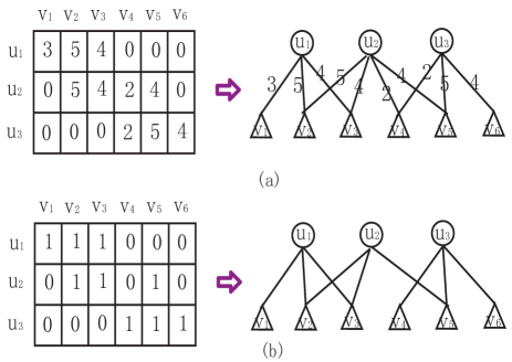
Figure 1: (a) Explicit rating matrix and the corresponding weighted bipartite graph, (b) Implicit preference matrix and the corresponding unweighed bipartite graph

For rating prediction problem, we are interested in finding the user neighbors and item neighbors in both modes of the graph simultaneously. For ranking-based recommendation, we are interested in finding the missing edges between the two partite indicating potential interests between user and item. Hereafter, we cast the CF problem as bipartite graph mining problem without special explanation.

2.3 Considering Time effects

The data in recommender systems keep changing. Not only new users and new items are continuously added to the system, the preferences of existing users and the features of existing items are also changing over time. To make better recommendations, algorithms should update the learned model efficiently and appropriately. By “efficiently” we mean the algorithm has the ability for fast or even real-time update. On the other hand, “appropriately” means we must take time factor into consideration when deciding on what to recommend to the users. For example, we can not expect users are equally satisfied with the recommendations of a very old movie and a brand new movie, even they have similar ratings.

In spite of its importance, time factors gain little attention in recommendation research area until recently. The authors of [16] proposed an incremental update method to compute the proximity of any two given nodes in the bipartite graph changing on the year base. [17] analyzed the evolution of ratings in the Netflix movie recommender system. It proposed two CF algorithms that consider time effects: item-item neighborhood method and rating matrix factorization method. Both the methods are elaboratively tailored for Netflix movie rating data and achieve the best results so far.

As pointed out in [17], preference evolution is subtle and delicate. For a single user, what we can use are often just a few preference instances inundated by millions of non-relevant data. The above mentioned methods have been designed and tested for special recommendation scenarios. However, in a more general sense, a robust recommendation algorithm considering time evolution for a wider range of applications including both rating-based and ranking-based recommender systems is still absent and is the main focus of our research.

3 Ant Collaborative Filtering

Before proceeding on a more detailed description, we first introduce notations and Ant Colony Algorithm which sheds some light on our proposed methods.

Table 1: Notations

Notation	Meaning
$u_{i}$, $v_{j}$	A user and an item
$r_{i,j}$	The rating that user $u_{i}$ gives to item $v_{j}$, $0$ if unknown
$\overline{r}$, $\overline{r}_{u_{i}}$, $\overline{r}_{v_{j}}$	The average rating for all the ratings, user $u_{i}$ and item $v_{j}$
$\mathscr{K}$, $K$	Total number of types of pheromone and maximum of types of pheromones attached to a user or an item, $\mathscr{K}\geq K$
$C(u_{i})$	Neighborhood user set for user $u_{i}$
$C(v_{j})$	Neighborhood item set for item $v_{j}$
$\mathbf{Ph(u_{i})}$, $\mathbf{Ph(v_{j})}$	The pheromones attached to user $u_{i}$ and item $v_{j}$, they are vectors of pheromones
$\gamma$, $\lambda$, $\sigma$	Parameters in our model, controlling the transmission rate, evaporating rate and disappearing rate
$TopN$	The recommenced top $N$ items
$Hitting$	The subset that user likes in the recommended list
$rank(v_{j})$	The final rank position for item $v_{j}$ in rank-based recommendation

3.1 Ant Colony Algorithm

Ant Colony Optimization (ACO) algorithms are proposed after observing the automatic accumulation or communication phenomena common to ant colony which thereafter have been widely applied in various domains such as clustering and information retrieval [11]. They belong to a more general group of simulation algorithms named swarm intelligence algorithms. In the typical settings of ACO, every ant is identified by some kind of indicators for communication often referred to as pheromone. The pheromone is used as an indirect communication medium. Taking Traveling Salesman Problem (TSP) which finds the shortest path on a graph for an example, while each ant walks on the graph, it leaves a pheromone signal through the path it used. Shorter paths will leave stronger signals. The next ants, when deciding which path to take, tend to choose paths with stronger signals with a higher probability, so that shorter paths are found.

ACO has several enticing properties. The most prominent one is that they are dynamic and self-organizing in nature. So it suits to solve the problems that are too complex and dynamic to be solved using other machine learning methods directly optimize some utility function.

There are applications of ACO in many information retrieval domains such as web search and social network. For example, [12] proposed a framework that models the web surfing activity as an ant colony group behavior. They took an analogy of users as ants and web pages as food. Similar analogy can be mapped onto users and items in the CF context.

3.2 Ant Collaborative Filtering

The intuition of our Ant Collaborative Filtering (ACF) algorithm is that given pheromone representing a user or a group of users, the item shares the user’s pheromone when she rates the item. Meanwhile, item transfers the pheromone already attached on it to the user. So after some time, similar items receive similar pattern of pheromone and then users with similar tastes become alike in respect to the pattern of pheromone on them. The pheromone transimission process is illustrated in Fig. 2, note that the ratings are learnt one by one in their original time order. Thus far, recommendation can be generated after two strategies: (1) Provided similar users and similar items found, we can estimate the current user’s rating on the items that she hasn’t seen before by simply employing memory based CF methods; (2) We can rank the items according to the similarity of its pheromones to the user’s. These two strategies correspond to rating-based and ranking-based recommendation mentioned above, respectively.

Figure 2: Pheromone transmission between users and items after several steps, the numbers in the circle indicate the timestamp, the triangles contain user pheromones and the rectangles contain item pheromones

3.2.1 Training

The training process is relatively simple and intuitive. Partial reason is that we need to retrain the model whenever there are new rating data available. In other words, our training process is incremental and is completed online.

First we initialize user pheromone by allocating every single user a unique pheromone with value $1.0$. The item pheromone is empty for every item. When a user $u_{i}$ gives a rating $r_{i,j}$ to item $v_{j}$, they exchange their pheromones, i.e., the user updates her pheromone by adding the item’s pheromones times by rating adjustment and a constant $\gamma$ which is introduced to control the spreading rate. For the item, similar update is computed. Because the bigger the gap between the rating and the average rating is, the stronger it bears user’s preference. If the rating is much higher than the average, the transmission will be a strong positive “plus”; on the other hand, if the rating is much less than the average, the transmission will be a strong negative “minus” which means the user and the item are not alike. So there are negative values for the pheromones.

As mentioned before, user’s interests change over time. Old interests fade out and new interests develop. We capture this evolution by the mechanism of pheromone evaporation. Before pheromone exchange between the user and the item, existing pheromones evaporate in a rate according the ratio of their amounts to the highest concentration among all the existing pheromones.

Therefore, for the rating-based recommendation scenario, the complete pheromone update formulae for the item and the user is described in Equ. (1) and Equ. (2).

$$\mathbf{Ph_{v_{j}}^{(t+1)}}=\mathbf{Ph_{v_{j}}^{(t)}}\times\exp\left(\frac{amount_{v_{j},k}+\lambda}{Max_{k\in K}(amount_{v_{j},k})+\lambda}-1\right)\\ +(r_{i,j}-\overline{r}_{u_{i}})\times\gamma\times\mathbf{Ph_{u_{i}}^{(t)}}$$ (1)

$$\mathbf{Ph_{u_{i}}^{(t+1)}}=\mathbf{Ph_{u_{i}}^{(t)}}\times\exp\left(\frac{amount_{u_{i},k}+\lambda}{Max_{k\in K}(amount_{u_{i},k})+\lambda}-1\right)\\ +(r_{i,j}-\overline{r}_{v_{j}})\times\gamma\times\mathbf{Ph_{v_{j}}^{(t)}}$$ (2)

For the 0/1 preference data, similarly, we rewrite the pheromone update formula as follows:

$$\mathbf{Ph_{v_{j}}^{(t+1)}}=\mathbf{Ph_{v_{j}}^{(t)}}\times\exp\left(\frac{amount_{v_{j},k}+\lambda}{Max_{k\in K}(amount_{v_{j},k})+\lambda}-1\right)\\ +\gamma\times\mathbf{Ph_{u_{i}}^{(t)}}$$ (3)

$$\mathbf{Ph_{u_{i}}^{(t+1)}}=\mathbf{Ph_{u_{i}}^{(t)}}\times\exp\left(\frac{amount_{v_{j},k}+\lambda}{Max_{k\in K}(amount_{u_{i},k})+\lambda}-1\right)\\ +\gamma\times\mathbf{Ph_{u_{i}}^{(t)}}$$ (4)

After evaporation and transmission, we delete the pheromones whose amount is less than our threshold $\sigma$ to keep our model simple and robust to rating noise. This process is referred to as threshold cut off. In our experiment, $\sigma$ is set to $0.01$. The training algorithm is shown below.

Input: $Ratings$, $U$, $V$

Output: Updated user pheromone and item pheromone

//Initialization

for $u_{i}\in U$  do

       $Ph_{u_{i}}^{(0)}=\{u_{i}:1.0\}$;

end for

for $v_{j}\in V$ do

       $Ph_{v_{j}}^{(0)}=\{\}$;

end for

//Training

for $rating\in Ratings$ do

       $u_{i}=rating[user]$;

       $v_{j}=rating[item]$;

       $value=rating[value]$;

       // Update user pheromones

       for $Pheromone\in\mathbf{Ph_{u_{i}}^{(t)}}$ do

             // Evaporation and Transmission

             $Pheromone=Pheormone\times\exp(\frac{amount_{Pheromone}+\lambda}{Max_{Ph_{u_{i}}}+\lambda}-1)+\gamma\times(value-\overline{r}_{v_{j}})\times Ph_{v_{j}}^{(t)}$

             // Cut off

             if $abs(Pheromone)<\sigma$ then

                   $Pheromone=0$;

             end if

            $\mathbf{Ph_{u_{i}}^{(t+1)}}\leftarrow Pheromone$;

       end for

      // Update item pheromones

       for $Pheromone\in\mathbf{Ph_{v_{j}}^{(t)}}$ do

             // Evaporation and Transmission

             $Pheromone=Pheromone\times\exp(\frac{amount_{Pheromone}+\lambda}{Max_{Ph_{v_{j}}}+\lambda}-1)+\gamma\times(value-\overline{r}_{u_{i}})\times Ph_{u_{i}}^{(t)}$

             // Cut off

             if $abs(Pheromone)<\sigma$ then

                   $Pheromone=0$;

             end if

            $\mathbf{Ph_{v_{j}}^{(t+1)}}\leftarrow Pheromone$;

       end for

      

end for

Algorithm 1 Training phase of ACF

3.2.2 Recommendation

We give recommendation algorithms for both explicit rating prediction and implicit relevance ranking tasks.

We can calculate the following three types of similarities though pheromone comparison:

• User-User similarity, $\mathbf{s(u_{i},u_{k})}$: to what extent any two given users $u_{i}$ and $u_{k}$ are alike, computed by comparison the user pheromones;

• Item-Item similarity, $\mathbf{s(v_{j},v_{l})}$: to what extent any two given items $v_{j}$ and $v_{l}$ are alike, computed by comparison the item pheromones;

• User-Item similarity, $\mathbf{s(u_{i},v_{j})}$: to what extent user $u_{i}$ and item $v_{j}$ are alike, computed by comparison the corresponding user and item pheromones.

For rating prediction, we employ memory based methods, i.e., using ratings from similar users to similar items to predict the current user $u_{i}$’s rating on current item $v_{j}$. The central problem is to find the best user neighbors and item neighbors that have similar rating patterns. In our experiments, the neighbor number is fixed as $20$ for both user neighbors and item neighbors. We first give rating-based recommendation in Alg. 2.

Input: $u_{i},v_{j},Ph(U),Ph(V)$

Output: $r_{i,j}$

// Find user neighbors

for $user\in U$ do

       $s_{u_{i},user}=\frac{\mathbf{Ph_{u_{i}}}\circ\mathbf{Ph_{user}}}{|\mathbf{Ph_{u_{i}}}|\times|\mathbf{Ph_{user}}|}$;

end for

// Sort users according to their similarity to the current // user in descendant order

$\mathbf{users}=sort(s_{u_{i},user})$;

$C(u_{i})=\mathbf{users}[0:Neighborhood\_size]$;

// Find item neighbors

for $item\in I$ do

       $s_{v_{j},item}=\frac{\mathbf{Ph_{v_{j}}}\circ\mathbf{Ph_{item}}}{|\mathbf{Ph_{v_{j}}}|\times|\mathbf{Ph_{item}}|}$;

end for

// Sort items according to their similarity to the current // item in descendant order

$\mathbf{items}=sort(s_{v_{j},item})$;

$C(v_{j})=\mathbf{items}[0:Neighborhood\_size]$;

// Fusing ratings

$user\_prediction=0;$

$user\_similarity=0;$

for $user\in C(u_{i})$ do

       if $user\ has\ rated\ item\ v_{j}$ then

             $user\_prediction\ +=abs(s(u_{i},user))*(r_{user,v_{j}}-\overline{r}_{user})$; $user\_similartity\ +=abs(s(u_{i},user))$;

       end if

      $user\_prediction\ /=user\_similarity$;

end for

$item\_prediction=0;$

$item\_similarity=0;$

for $item\in C(v_{j})$ do

       if $u_{i}\ has\ rated\ item$ then

             $item\_prediction\ +=abs(s(item,v_{j}))*(r_{u_{i},item}-\overline{r}_{item})$; $item\_similartity\ +=abs(s(item,v_{j}))$;

       end if

      $item\_prediction\ /=item\_similarity$;

end for

$prediction=\overline{r}+user\_prediction+item\_prediction;$

Algorithm 2 Rating-based recommendation

On the other hand, relevance ranking task concerns about how relevant that the current user and an item are. This problem equals to ranking the items according to their similarities to the current user. The detailed algorithm is shown in Alg. 3.

Input: $u_{i},Ph(U),Ph(V)$

Output: Recommendation list

// Calculate user-item similarities

for $item\in I$ do

       $s(u_{i},item)=\frac{\mathbf{Ph_{u_{i}}}\circ\mathbf{Ph_{item}}}{|\mathbf{Ph_{u_{i}}}|\times|\mathbf{Ph_{item}}|}$;

end for

// Ranking

$\mathbf{return}$ $Top\ N$ list of items ranked by $s(u_{i},item)$ in descendant order

Algorithm 3 Ranking-based recommendation

4 Ant Collaborative Filtering with Dimension Reduction

In the previous section, we have explained the basic Ant Collaborative Filtering algorithm. Taking one step further to solve the sparsity problem, we try to improve the ACF by introducing dimension reduction technique into our previous scheme.

4.1 Dimension Reduction Version for ACF

In Algorithm ACF, for every single user we allocate a unique type of pheromone. Since we intend to represent preference patterns using different pheromones, much less types of pheromones are actually needed. We can reduce the number of types of pheromones and thus can help alleviate sparsity problem. This improved version of ACF is named IACF.

We first cluster the users into $\mathscr{K}$ clusters according to their rating pattern, where $\mathscr{K}$ is the desired number of types of pheromones. Because user clustering is for pheromone initialization and principally we can use various clustering techniques [22]. We have tested several clustering methods such as K-means and spectral clustering. We implemented these two methods and found K-means is more suitable for our dataset because it generated more balanced clusters. Without special explantation, we use K-means as initialization process in our following IACF algorithms.

The detailed IACF algorithm is shown in Alg. 4. The difference between ACF and IACF is in their pheromone initialization phase, the rest of the algorithm is kept unchanged as Alg. 1.

Input: $Ratings$, $U$, $V$, $\mathscr{K}$

Output: Updated user pheromone and item pheromone

// Clustering users

Cluster users into $\mathscr{K}$ clusters according to their rating patterns using K-means;

//Initialization

for $user\in U$ do

       // The user belongs to cluster $k$

       $\mathbf{Ph_{user}}=\{Pheromone_{k}:1.0\}$;

end for

for $item\in I$ do

       $\mathbf{Ph_{item}}=\{\}$;

end for

// The rest of the algorithm is the same as Alg. 1

Algorithm 4 IACF training algorithm

4.2 Complexity Analysis

For batched training phase the time complexities for both ACF and IACF are $O(K\times\#ratings)$, where $K$ is the maximum number of types of pheromones that a user and item carry for both ACF and IACF. Typically, we have $k<<\#users$. For online update, the update complexity is only $O(K)$. Generally speaking, IACF is a little faster because typically there are less types of pheromones attached to the user and item.

In the recommendation phase, for the rating-based recommendation, the time complexity is $O(\#users+\#items)$, but the computations could be significantly reduced if we maintain user neighbors and item neighbors explicitly in memory or in database. For the ranking-based recommendation, the time complexity is $O(\#items)$. This is the lower bound for the recommendation algorithms because we must scan all the item list before generating a $TopN$ recommendation list.

5 Related Works

5.1 Bipartite Graph based Collaborative Filtering

Modeling data mining task as a bipartite graph analysis problem has a long tradition. [3] might be the earliest work that applied graphic analysis technique in CF recommendation. Comparing with one mode graph, it is more natural and precise to model CF problem as a bipartite graph with users and items as two disjoint groups of nodes. The methods following this direction CF based on generally fall into three categories: spectral analysis of the associated matrix, random walks and Activation Spreading.

[21] introduced bipartite graph co-clustering algorithm based on the usage the second smallest eigenvector of the associated matrix of the graph. It achieves the optimal clustering results in the sense of minimization the cuts of edges between any two clusters. [14] followed this direction and applied this technique on the task of finding missing links in a movie rating bipartite graph.

The most well known bipartite graph algorithm in Information Retrieval may be HITS [20] proposed in 1998. It calculates the stationary status of both groups of nodes through mutual reinforcement on the bipartite graph. It is a typical random walk method on the bipartite graph. Similar works include [9] and [6]. [6] try to find most relevant users using the user-item Bipatite graph which recommendations are generated upon. Interestingly, [10] links the random walks methods and spectral based methods. Actually, spectral methods are often implemented using random walks iterations.

Another important technique in graph mining is Activation Spreading (AS) which models the relationships among the nodes in the graph through iteratively propagation of activation value. [8] surveyed several AS methods and compared them on a CF task. Their conclusion is that Hopfield net algorithm outperforms others on their book recommendation data set. [7] applied AS technique on rating-based CF and proposed a novel HITS-like CF algorithm: RSM. We will compare it with our proposed ACF algorithm in the experiments. In addition, ACF can also be viewed as a AS extension in recommender systems, the major difference is that we view the Bipartite user-item relationship as a dynamic network and learn the training data incrementally.

The underline principal of the latter two categories is to use smooth techniques to alleviate the insufficiency of known value of either the vertices or the edges. This direction is specially important for collaborative filtering because of sparsity of rating data.

5.2 Dimension Reduction in Collaborative Filtering

Finding a lower rank representation of the original rating data is an often used way to combat sparsity. The bulk of model based collaborative filtering are dimension reduction methods in their essence. The underlying reason is there are much fewer factors than the dimension of the rating data that actually govern users’ choices. So in practice, dimension reduction can improve both the performance and efficiency of recommendation algorithms.

Model based recommendation algorithms include probabilistic methods and matrix factorization methods. The probabilistic methods assume there are some latent topics that both the users and the items belong to. The crux is to learn these probabilities that similar users and similar items are in similar topics. Probabilistic Latent Semantic Analysis (PLSA) [25] is one of such algorithms. Another model-based algorithm, Non-negative Matrix Factorization (NMF) [26] belongs to the matrix factorization methods that also have many extensions and applications in CF domain. By restricting the rank of the factorized matrices as the user profile and item profile, these methods are themselves the well known dimension reduction techniques and are considered to be the state-of-art of CF algorithms [17].

5.3 Swarm Intelligence Recommendation

To our best knowledge, there are few works that directly related to our model in the CF domain. But in a more general sense, several swarm intelligence algorithms have been applied to recommendation tasks.

[18] applied heat diffusion model on online advertisement task. The basic idea is that heat always flows from a position with high temperature to a position with low temperature. Influence transmission between friends in a social network is similar to this diffusion process. [19] used particle swarm optimization algorithm to model every user as a particle in a multi-dimensional space with each dimension representing a movie genre. Its advantage is that every particle have a unique position and velocity, so the system is dynamic and to a certain extent probabilistic in nature, which is preferable in recommender systems.

5.4 Comparing with ACF

Through the analysis above, we can see the relationships between ACF and other existing methods including bipartite graph based and swarm intelligence based CF methods especially Activation Spreading algorithms. The improvements of ACF are three-fold: (1) Comparing with Activation Spreading algorithms, because of the mechanism of pheromone evaporation we don’t have over-spreading problem which results in too strong relationship between users and items to find high quality neighbors; (2) Our training process is performed online and in accordance with the real time sequence of the user preferences; (3) Both rating-based and ranking-based algorithms are considered. For the systems with both two types of preference data like Amazon and Douban, these two methods can be complement to each other.

6 Experiments

As mentioned in Section 2.1, collaborative filtering methods follow either of two different strategies: rating prediction and top-N ranking. We experiment our proposed methods on both of two different scenarios.

6.1 Rating-based Recommendation

We experiment the rating prediction algorithms on a popular movie recommendation dataset: MovieLens (http://www.grouplens.org/node/73). The MovieLens data we use consist of $1,000,000$ ratings from $6,040$ users on $3,706$ movies. Ratings are made on a five-star scale. Of these ratings, $90\%$ are used for the model training, and the rest $10\%$ constitute test set.

The evaluation metric is Root Mean Square Error (RMSE) as follows (the smaller, the better):

$$RMSE=\sqrt{\frac{1}{n}\sum_{(u_{i},v_{j})\in TestSet}(r_{i,j}-estimated\_rating)^{2}}.$$

We have some parameters in our algorithm, namely transmission rate $\gamma$, evaporation rate $\lambda$ and the cluster number for IACF to be tuned. The transmission rate $\gamma$ controls the speed of pheromones that are transferred from the user to the item and vice versa. The bigger, the faster the pheromones transmit. The evaporation rate $\lambda$ controls the speed of the pheromone evaporation both on users and items. Bigger value results in slower evaporation, which means weaker time influences in recommendation. In our experiments, $\gamma$ is set to be $0.2$ and $\lambda$ is 1. For IACF, the cluster number is $20$.

We compare our proposed methods with two memory based methods: classic user-based CF and item-based CF [23], two model based methods: Probabilistic Latent Semantic Analysis (PLSA) [25], Non-negative Matrix Factorization (NMF) [26] and an Activation Spreading method: RSM [7]. The comparison results are shown in Table 2.

Table 2: Rating Results Evaluation

Algorithm	RMSE	Time (s)
User-based	$0.993\pm 0.02$	$98.5$
Item-based	$0.979\pm 0.01$	$1990.0$
NMF	$1.127\pm 0.05$	$1605.0$
PLSA	$1.093\pm 0.02$	$102541.0$
RSM	$1.016\pm 0.02$	$581.0$
ACF	$1.008\pm 0.03$	$85.4$
IACF	$\mathbf{0.953\pm 0.03}$	$\mathbf{60.2}$

Although MovieLens data have timestamp information attached to each rating, we don’t consider time effects because the timestamp don’t reflect the evolving of user interests at all. So all the algorithms are trained in a batched fashion without special time consequence. We will see the influences of time in the following experiments.

6.2 Ranking-based Recommendation

In order to evaluate the performance of our method on ranking-based recommendation scenario, we experiment our ranking-based recommendation algorithm on two real-world recommender systems: book recommendation and music recommendation. The book recommendation data are crawled from the largest Chinese book recommendation website: Douban (http://www.douban.com). For experiment, we use part of the readers and books as our training/testing dataset. The music recommendation data are crawled from the largest online music recommender system: Last.FM (http://www.last.fm). We use these two datasets because: (1) they are of higher quality than experimental dataset in terms of reflecting real user preferences; (2) they symbolize two types of popular recommender systems; (3) they both contain time information in their implicit ratings that we are interested in. Table 3 shows some statistics of the datasets.

Table 3: Dataset Properties

	Douban	Last.FM
#User	$124$	$675$
#Item	$14843$	$8010$
#Preference	$24862$	$14007$
Time Span	$2005.3.7\sim 2009.6.22$	$2006.3.3\sim 2009.6.22$
Sparsity	$98.65$%	$99.74$%

However, one of the flaws for ranking-based recommendation is lack of evaluation metrics as effective as rating-based recommendation. In order to be less subjective, we use two metrics: Precision [1] and Ranking Accumulation (RA) [4] defined as follows.

$$Precision=\frac{\#\ Hitting}{N},$$

$$RA=\sum_{item\in Hitting}\frac{rank(item)}{N}+\sum_{item\not\in Hitting}\frac{N+1}{N}.$$

Apparently, $Precision\in[0,1]$, the higher the better; $RA\in[\frac{N+1}{2},N+1]$, and smaller value is better. (Note that the $Hitting$ set only contains the items that both are interesting to the user and already in our test set. So the measured precision and ranking accumulation both underestimates the real performance.) We compare our methods with the three ranking-based CF methods reported in [4, 7, 1] respectively together with classic user-based and item-based CF algorithms. The methods proposed in [4] and [7] belong to the general Activation Spreading and are denoted as NBI and RSM , respectively. We also implemented the BM25-Item algorithm in [1]. Similarly, we hold $10\%$ data for testing. All the results are obtained by averaging 5 different runs. The comparison results are shown in Table 4 below.

Table 4: Ranking Results Comparison

Dataset	Algorithm	Precision	RA	Time (s)
	User-based	$0.045$	$20.415$	$\mathbf{17.5}$
	Item-based	$0.006$	$20.923$	$155.7$
	NBI	$0.002$	$20.966$	$928.0$
Douban	RSM	$0.035$	$20.571$	$27.2$
	BM25-Item	$0.014$	$20.850$	$202.0$
	ACF	$0.062$	$20.320$	$31.1$
	IACF	$\mathbf{0.065}$	$\mathbf{20.231}$	$29.4$
	User based	$0.050$	$20.386$	$\mathbf{6.4}$
	Item based	$0.040$	$20.433$	$84.6$
	NBI	$0.003$	$20.957$	$255.7$
Last.FM	RSM	$0.049$	$20.356$	$18.4$
	BM25-Item	$0.028$	$20.726$	$219.8$
	ACF	$0.076$	$20.102$	$25.1$
	IACF	$\mathbf{0.081}$	$\mathbf{19.915}$	$22.3$

For all the algorithms in the above experiments we use batched training data without considering time influence. Since the personalize recommendations such as book and music recommendation performances are heavily depending on the time, results can be further improved by updating our IACF model using preference data in their original time order. The IACF with and without considering time sequence are referred to as time and timeless version. We choose 15 time points within the time span, denoted as $1\sim 15$ from $2006.3.3$ to $2009.6.22$. The results are shown in the Fig. 3. From the results we could see a clear increase of precision as time goes on. It means when users keep using our recommender systems, the recommendation will be more and more accurate.

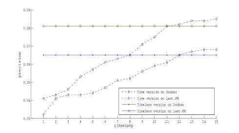
Figure 3: Precision comparison of time and timeless versions for IACF on the Douban and Last.FM dataset

7 Conclusion and Future Works

Recommendation is becoming of more importance for many Internet services. We have seen plenty of researches concerning on improving the accuracy of recommendation algorithms on static, rating-based data. But as pointed out in the very recent paper [17], improved accuracy is not a panacea, there are also other challenges for collaborative filtering. Scalability is one of most mentioned concerns and time effects are also a indispensable factor to be considered in dynamic recommender systems. In this paper, we proposed a novel CF algorithm inspired by the ant colony behavior. By pheromone transmission between users and items and evaporation of those pheromones on both users and items over time, ACF could flexibly reflect the latest user preference and thus make most reliable recommendations.

In a nutshell, our major contributions are:

• It introduced the concepts in Ant Colony Optimizations (such as Pheromone, Evaporation and etc.) into recommendation domain and proposed an incremental, scalable collaborative filtering algorithm that can nicely handle sparse and evolving rating data;

• It fused dimension reduction with the Ant Collaborative Filtering algorithm above mentioned;

• The algorithm proposed in this paper could recommend with both strategies: rating-based and ranking-based recommendation which are used in explicit user preference and implicit user preference scenarios respectively;

• Last but not least, ACF algorithm is easy to be deployed on distributed computational resources, even in a Peer-to-peer environment, which means a higher scalability and more importantly, user privacy protection.

There are also some unexplored possibilities to improve the algorithm proposed in this paper. First, the initialization of pheromones does affect the final recommendation results as shown in the dimension reduction version of ACF. There may be other initialization schemes that we can make further improvements. Second, evaporation is an interesting while hard-to-tune mechanism that applications should find the most suitable rate to their own needs. Last but not least, Bipartite based ranking methods including ours are flexible and can often fuse user preference data other than user ratings [5]. This is also a promising direction.

8 Acknowledgements

We thank State Key Laboratory of Computer Science for subsidizing our research under the Grant Number: CSZZ0808, the National Science and Technology Major Project under Grand Number:2010ZX01036-001-002-2 and the Grand Project Network Algorithms and Digital Information of the Institute of Software, Chinese Academy of Sciences under Grant Number:YOCX285056.

References

- [1] J. Wang, S. Robertson, A.P. De Vries, and M.J.T. Reinders. Probabilistic relevance ranking for collaborative filtering. In Information Retrieval 11(6): 477-497, 2008.
- [2] B. Marlin. Collaborative Filtering: A Machine Learning Perspective. Master’s thesis, University of Toronto, 2004.
- [3] C.C. Aggarwal, J.L. Wolf, K.-L. Wu, and P.S. Yu. Horting Hatches an Egg: A New Graph-Theoretic Approach to Collaborative Filtering. In Proceedings of the Fifth ACM SIGKDD: 201-212, 1999.
- [4] T. Zhou, J. Ren, M. Medo, and Y. Zhang. Bipartite network projection and personal recommendation. In Physical Review E (Statistical, Nonlinear, and Soft Matter Physics), 76(4), 2007.
- [5] H.B. Deng, M.R. Lyu, and I. King. A Generalized Co-HITS Algorithm and Its Application to Bipartite Graphs. In Proceedings of the 15th ACM SIGKDD Conference on Knowledge Discovery and Data Mining, 2009.
- [6] B.J. Mirza, B.J. Keller, and N. Ramakrishnan. Studying Recommendation Algorithms by Graph Analysis. In Journal of Intelligent Information Systems 20(2): 131-160, 2003.
- [7] P. Han, B. Xie, F. Yang, and R.M. Shen. An Adaptive Spreading Activation Scheme for Performing More Effective Collaborative Recommendation. In Proceeding of International conference on database and expert systems applications: 95-104, 2005.
- [8] Z. Huang, H. Chen, and D. Zeng. Applying Associative Retrieval Techniques to Alleviate the Sparsity Problem in Collaborative Filtering. In ACM Transactions on Information Systems 22(1): 116-142, 2004.
- [9] N. Craswell, and M. Szummer. Random Walks on the Click Graph. In Proceedings of the 30th annual international ACM SIGIR conference: 239 - 246, 2007.
- [10] Marina Meila, Jianbo Shi. Learning Segmentation by Random Walks. In Proceedings of Advances in Neural Information Processing Systems: 873-879, 2000.
- [11] M. Dorigo. Optimization, Learning and Natural Algorithms. Ph.D.Thesis, Politecnico di Milano, Italy, 1992.
- [12] J. Wu, and K. Aberer. Swarm Intelligent Surfing in the Web. In Proceedings of International Conference on Web Engineering: 277-284, 2003.
- [13] B. Eric, D. Marco, and T. Guy. Swarm intelligence: from natural to artificial systems. Oxford University Press, New York, NY, USA, 1999.
- [14] T. Liu, Y.H. Tian, and W. Gao. A Two-Phase Spectral Bigraph Co-clustering Approach for the ”Who Rated What” Task in KDD Cup 2007. In Proceedings of ACM KDDCup.07: 63-68, 2007.
- [15] J.F. Pessiot, V. Truong, and etc. Learning to Rank for Collaborative Filtering. In Proceedings of International Conference on Enterprise Information Systems: 145-151, 2007.
- [16] H.H. Tong, S. Papadimitriou, P.S. Yu, and C. Faloutsos. Proximity Tracking on Time-Evolving Bipartite Graphs. In SIAM, 2008.
- [17] Y. Koren. Collaborative Filtering with Temporal Dynamics. In Proceedings of 15th ACM SIGKDD Conference, 2009.
- [18] H. Ma, H.X. Yang, M.R. Lyu, and I. King. Mining Social Networks Using Heat Diffusion Processes for Marketing Candidates Selection. In Proceeding of the 17th CIKM Conference: 233-242, 2008.
- [19] S. Ujjin, and P.J. Bentley. Particle Swarm Optimization Recommender System. In Proceeding of the IEEE Swarm Intelligence Symposium: 124-131, 2003.
- [20] J. Kleinberg. Authoritative Sources in a Hyperlinked Environment. In Proceedings of the ACM-SIAM Symposium on Discrete Algorithms: 668-677, 1998.
- [21] I.S. Dhillon. Co-clustering Documents and Words using Bipartite Spectral Graph Partitioning. In Proceeding of ACM SIGKDD: 269-274, 2001.
- [22] Rui Xu, Wunsch, D..Survey of clustering algorithms. IEEE Transactions on Neural Networks, 16(3): 645-678, 2005.
- [23] B. Sarwar, G. Karypis, J. Konstan, and J. Riedl. Item-based collaborative filtering recommendation algorithms. In Proceedings of the 10th WWW Conference: 285-295, 2001.
- [24] G. Karypis. Evaluation of Item-Based Top-N Recommendation Algorithms. In Proceedings of the 10th CIKM Conference: 247-254, 2001.
- [25] T. Hofmann. Latent Semantic Models for Collaborative Filtering. In ACM Transaction Information System 22(1): 89-115, 2004.
- [26] S. Zhang, W.H. Wang, J. Ford, F. Makedon. Learning from Incomplete Ratings Using Non-negative Matrix Factorization. In 6th SIAM Conference on Data Mining : 548-552, 2006.
- [27] A. Das, M. Datar, A. Garg, and S. Rajaram. Google News Personalization: Scalable Online Collaborative Filtering. In Proceedings of the 16th WWW Conference: 271-280, 2007.
- [28] J. Ben Schafer, Joseph A. Konstan, John Riedl. E-Commerce Recommendation Applications. Data Mining and Knowledge Discovery, Vol. 5 (1-2), 2001:115-153.