Gauge invariants of eigenspace and eigenvalue anholonomies: Examples in hierarchical quantum circuits

Abstract

A set of gauge invariants are identified for the gauge theory of quantum anholonomies, which comprise both the Berry phase and an exotic anholonomy in eigenspaces. We examine these invariants for hierarchical families of quantum circuits whose qubit size can be arbitrarily large. It is also found that a hierarchical family of quantum circuits generally involves an NP-complete problem.

1 Introduction

An adiabatic time evolution of a quantum system along a closed loop may induce a nontrivial change. The best known among them is the phase anholonomy, which is also referred to as the Berry phase: a stationary state acquires an extra phase of geometrical origin as a result of an adiabatic cycle [1]. It has been recognized that the eigenvalue and eigenspace of a bound state can be also changed by an adiabatic cycle [2]: When we keep track of an eigenvalue along a cycle, discrepancies may appear between the initial and finial eigenvalues. Such a change, which is called an eigenvalue anholonomy, implies the interchange of the eigenvalues, which is in fact allowed because of the periodicity of the spectrum for the cycle. Furthermore, due to the correspondence between eigenvalues and eigenspaces, the eigenvalue anholonomy implies the eigenspace anholonomy, where an adiabatic cycle delivers one stationary state into another stationary state.

The earliest example of the eigenvalue and eigenspace anholonomies is found in a family of Hamiltonians with generalized point interactions [3]. Later, it is recognized that there is another examples of anholonomy in Hamiltonian systems that involve crossings of eigenenergies [4, 5]. Further examples are found recently in periodically driven systems and quantum circuits, where a stationary state is an eigenvector of a unitary operator that describes the evolution for a unit time interval [6, 7, 8]. The spectral degeneracies are known to make both the phase anholonomy [9] and the eigenspace anholonomies more interesting. However, throughout this paper, we will focus on the case where no spectral degeneracy exists along adiabatic cycles.

We have recently developed a unified gauge theoretic formalism of eigenspace anholonomy [10], extending the Fujikawa’s approach to the phase anholonomy [11]. The key quantity for the formalism is the holonomy matrix $M(C)$, whose elements are given by overlapping integrals between stationary states and their adiabatic transports along a cyclic path $C$. Because $M(C)$ is gauge covariant  [10], only a part of $M(C)$ is observable [12].

In this paper, we show how we extract gauge invariants from $M(C)$. Let us suppose that all stationary states in $N$-dimensional Hilbert space are connected by the $N$-repetition of the adiabatic cycle. It can be shown that $M(C)$, under an appropriate choice of the gauge, is given in terms of two gauge invariants $\mathfrak{S}(C)$ and $\gamma(C)$:

$$M(C)=\mathfrak{S}(C)\,\rme^{\rmi{}\gamma(C)/N},$$ (1)

where $\mathfrak{S}(C)$ is a permutation matrix that describes the interchange of eigenspaces induced by the adiabatic cycle $C$, and $\gamma(C)$ is the Berry phase gained through the $N$-repetition of the cycle $C$. In general, $M(C)$ is decomposed into the blocks, each of which consists of a permutation matrix and a geometric phase factor as shown in (1).

Also, in this paper, we provide examples of systems that exhibit various types of $\mathfrak{S}(C)$ by extending a recursive construction of hierarchical quantum circuits [8]. Due to its topological nature, $\mathfrak{S}(C)$ remains unchanged under small perturbations, and the eigenspace and eigenvalue anholonomy with various $\mathfrak{S}(C)$ are robust against small imperfections inevitable in experimental implementation.

The plan of this paper is the following. We first lay out the concept of the eigenspace and eigenvalue anholonomies with the minimal model, a quantum circuit on a qubit, in Section 2. In Section 3, we revisit our gauge theoretic formalism [10] to reveal the hidden gauge invariants $\mathfrak{S}(C)$ and $\gamma(C)$ residing in $M(C)$. In the following sections, we attempt to extend the recursive construction of quantum circuits [8] in order to obtain expanded instances of families of systems with variety of $\mathfrak{S}(C)$. In Section 4, we introduce novel families of quantum circuits. The eigenvalue problem of these circuits are also solved. In Section 5, we examine the eigenvalue anholonomy of our hierarchical models, and obtain $\mathfrak{S}(C)$ for each family of quantum circuits. In Section 6, we examine the eigenspace anholonomy of the hierarchical models to obtain $\gamma(C)$ hidden in $M(C)$. In Section 7, several examples are shown. We examine the relationship between our model and the adiabatic quantum computation [13] along the eigenangle [14] in Section 8. In Section 9, we discuss the relationship between our result and a topological characterization of the winding of quasienergies for periodically driven systems [15]. A summary of this paper is found in Section 10. Several technical details are provided in an Appendix.

2 Anholonomies in quantum circuits

We lay out the eigenvalue and eigenspace anholonomies and associated gauge invariants using a family of quantum circuits on a qubit. These quantum circuits provide the simplest case for our analysis shown in latter sections.

We introduce a quantum circuit on a qubit, or, equivalently a quantum map for spin-$\frac{1}{2}$ [10, 16]:

$$\hat{u}(\lambda,p)\equiv\exp\left\{\rmi{}(p-1)\lambda(1-|{}y{}\rangle\langle{}y{}|)+\rmi{}\lambda|{}y{}\rangle\langle{}y{}|\right\}\hat{Z},$$ (2)

where $p$ is an integer. Using orthonormal vectors $|{}0{}\rangle$ and $|{}1{}\rangle$ of the qubit, we define $|{}y{}\rangle\equiv(|{}0{}\rangle-i|{}1{}\rangle)/{\sqrt{2}}$ and $\hat{Z}\equiv|{}0{}\rangle\langle{}0{}|-|{}1{}\rangle\langle{}1{}|$. Because $\hat{u}(\lambda,p)$ is $2\pi$-periodic in $\lambda$, we will examine the eigenvalue and eigenspace anholonomies for the cycle $C$, for which $\lambda$ is increased from $0$ to $2\pi$. We denote an eigenvalue of the unitary operator $\hat{u}(\lambda,p)$ as $\exp\{i\theta(n;\lambda,p)\}$, where an eigenangle $\theta(n;\lambda,p)$ satisfies

$$\theta(n;\lambda,p)=n\pi+\frac{p}{2}\lambda,$$ (3)

for $n=0,1$. The corresponding eigenvectors are the following:

$$|{}0(\lambda,p){}\rangle =|{}0{}\rangle\cos\frac{(2-p)\lambda}{4}+|{}1{}\rangle\sin\frac{(2-p)\lambda}{4},$$ (4a)

$$|{}1(\lambda,p){}\rangle =|{}1{}\rangle\cos\frac{(2-p)\lambda}{4}-|{}0{}\rangle\sin\frac{(2-p)\lambda}{4}.$$ (4b)

First, we examine an anholonomy in the eigenangle $\theta(n;\lambda,p)$. As $\lambda$ is increased from $0$ to $2\pi$ along the closed cycle $C$, we obtain the following change

$$\theta(n;\lambda+2\pi,p)=\theta(s(n;C);\lambda,p)+2\pi r(n;C),$$ (4e)

where we introduce integers

$$s(n;C)\equiv(n+p){{\rm\ mod\ }2},\quad r(n;C)\equiv\left[({n+p})/{2}\right],$$ (4f)

and $[x]$ is the maximum integer less than $x$. Hence, when $p$ is even, $n$-th eigenangle is transported to itself by the cycle $C$. On the other hand, odd $p$ implies the presence of an anholonomy in the eigenangles, i.e., $\theta(n;\lambda+2\pi,p)=\theta(\bar{n};\lambda,p)+2\pi n$, where $\bar{0}=1$ and $\bar{1}=0$.

The eigenangle anholonomy implies an anholonomy in eigenspaces. Namely, the adiabatic transport of an eigenspace along the cycle $C$ induces the change in eigenvectors. Suppose that each eigenvector $|{}n(\lambda,p){}\rangle$ satisfies the parallel transport condition within the eigenspace [17], i.e.,

$$\langle{}n(\lambda,p){}|\left[\partial_{\lambda}|{}n(\lambda,p){}\rangle\right]=0.$$ (4g)

This condition is, in fact, satisfied by the eigenvectors (4a) and (4b). The adiabatic cycle $C$ accordingly transports $|{}n(0,p){}\rangle$ to $|{}n(2\pi,p){}\rangle$. Because of the correspondence between the eigenangle and the eigenspace, $|{}n(2\pi,p){}\rangle$ must agree with $|{}s(n;C)(0,p){}\rangle$ up to a phase factor. When $p$ is odd, $|{}n(2\pi,p){}\rangle$ is orthogonal to $|{}n(0,p){}\rangle$ because of $s(n)\neq n$. Note that the change of the eigenvector occurs in spite of the absence of the spectral degeneracy along the path $C$. Hence this anholonomy is different from Wilczek-Zee’s phase anholonomy. Instead, an anholonomy appears in the eigenspace.

The change in the eigenvectors is characterized by the overlapping integrals between the initial and the finial eigenvector

$$\{M(C)\}_{n^{\prime},n}\equiv\langle{}n^{\prime}(0,p){}|{}n(2\pi,p){}\rangle,$$ (4h)

which we call a holonomy matrix. This involves the interchange of eigenspaces and the accumulation of phases. Although we have assumed the parallel transport condition for each eigenspace in (4h), $M(C)$ is gauge covariant with respect to the gauge transformation for $|{}n(\lambda,p){}\rangle$, as will be explained in Section 3 [10]. Due to the gauge covariance, only a part of $M(C)$ is observable [12].

We now look for the gauge invariants, i.e. observables, of the quantum anholonomies for the adiabatic cycle $C$. They can be identified easily by investigating $M(C)$ closely. One is the permutation matrix $\mathfrak{S}(C)$:

$$\{\mathfrak{S}(C)\}_{n^{\prime},n}\equiv\delta_{n^{\prime},s(n;C)},$$ (4i)

which reflects the interchange of eigenvalues and eigenspaces. Other gauge invariants are the geometric phases. When $M(C)$ is diagonal, i.e., the eigenspace and eigenvalue anholonomies are absent, the $n$-th diagonal element of $M(C)$ is the Berry phase for the $n$-th eigenspace. On the other hand, if the eigenspace and eigenvalue anholonomies occur, $M(C)$ contains the off-diagonal geometric phases, which have been introduced to quantify the phase anholonomy for a noncyclic-path [18] under the presence of the eigenspace interchange [19].

Let us look at the holonomy matrix and the gauge invariants in our model (2). Since eigenvectors (4a) and (4b) satisfy the parallel transport condition (4g), we obtain

$$M(C)=1\cos\frac{\pi(2-p)}{2}-iY\sin\frac{\pi(2-p)}{2},$$ (4j)

where $1$ is the identity matrix (which will be omitted below) and

$$Y=\left(\begin{array}[]{cc}0&-i\\ i&0\end{array}\right).$$ (4m)

Because the integer $p$ is a crucial parameter for the anholonomies as shown above, it is better to classify the cases depending on whether $p$ is even and odd to investigate the gauge invariants. When $p$ is even, we obtain $s(n;C)=n$ for $n=0$ or $1$. Namely the anholonomies apparently disappear, i.e.,

$$\mathfrak{S}(C)=\left(\begin{array}[]{cc}1&0\\ 0&1\end{array}\right).$$ (4p)

The permutation described by $\mathfrak{S}(C)$ consists of two disconnected cycles each of which has a unit length. The holonomy matrix takes block-diagonal form, whose diagonal blocks are two $1\times 1$ matrices, i.e.,

$$M(C)=\left(\begin{array}[]{cc}\sigma(0;C)&0\\ 0&\sigma(1;C)\end{array}\right),$$ (4s)

where $\sigma(n;C)\equiv(-1)^{(2-p)/2}$ is the Berry phase factor acquired through the adiabatic cycle $C$ for the $n$-th eigenspace.

On the other hand, odd $p$ implies $s(0;C)=1$ and $s(1;C)=0$. Hence the eigenvalue and eigenspace anholonomies appear explicitly, i.e.,

$$\mathfrak{S}(C)=\left(\begin{array}[]{cc}0&1\\ 1&0\end{array}\right),$$ (4v)

which is the permutation matrix of the cycle whose length is $2$. The holonomy matrix can be regarded as a product of $\mathfrak{S}(C)$ and a diagonal unitary matrix, i.e.,

$$M(C)=\mathfrak{S}(C)\left(\begin{array}[]{cc}\sigma(0;C)&0\\ 0&\sigma(1;C)\end{array}\right),$$ (4y)

where we set $\sigma(n;C)\equiv(-1)^{n+(1-p)/2}$. Each $\sigma(n;C)$ has no geometric significance since it depends on the choice of the gauge. We can thus construct a gauge invariant quantity $\sigma(0;C)\sigma(1;C)=-1$. This is the Manini-Pistolesi’s off-diagonal geometric phase factor, which is an extension of Berry’s phase factor for the case that the permutation of eigenvectors takes place along an adiabatic evolution [19]. Once we slightly change the phase of eigenvectors as $|{}\tilde{0}(\lambda,p){}\rangle\equiv\rmi|{}0(\lambda,p){}\rangle$ and $|{}\tilde{1}(\lambda,p){}\rangle\equiv|{}1(\lambda,p){}\rangle$, the holonomy matrix in the corresponding gauge takes a canonical form, i.e.,

$$\tilde{M}(C)=\mathfrak{S}(C)\,\rme^{\rmi\gamma(C)/2},$$ (4z)

where $\gamma(C)=\pi p$ agrees with the Manini-Pistolesi off-diagonal geometric phase, up to a modulo $2\pi$.

So far, we have examined specific families of quantum circuits, namely $\hat{u}(\lambda,p)$ (2) with $|{}y{}\rangle=(|{}0{}\rangle-\rmi|{}1{}\rangle)/{\sqrt{2}}$ and $\hat{Z}=|{}0{}\rangle\langle{}0{}|-|{}1{}\rangle\langle{}1{}|$. This analysis can be applied to the whole family of $\hat{u}(\lambda,p)$ with arbitrary $|{}y{}\rangle$ and $\hat{Z}$. For the path $C_{p}$ of the whole family $\hat{u}(\lambda,p)$, $C_{p}$ still has topological invariant, namely either (4p) or (4v). Although we may deform the closed path $C_{p}$ by varying $|{}y{}\rangle$ and $\hat{Z}$ in $\hat{u}(\lambda,p)$, the topological invariant $\mathfrak{S}(C)$ remains intact unless the deformed path encounters a spectral degeneracy. Hence, for every path $C$ obtained by deforming $C_{p}$ with even $p$, $\mathfrak{S}(C)$ is the unit matrix. With odd $p$, $\mathfrak{S}(C)$ is always the permutation matrix of the cycle whose length is $2$. Hence the closed paths are divided into two families related to the value of $\mathfrak{S}(C)$, i.e. the unit or the permutation matrix except the paths that come across spectral degeneracies.

3 Gauge invariants of the quantum anholonomy

In this section, we first review our unified gauge theoretical treatment of quantum anholonomy that is applied both to the Berry phase and the eigenspace anholonomy [10, 16]. This offers a gauge covariant expression of the holonomy matrix $M(C)$ using a non-Abelian gauge connection. Second, we reveal gauge invariants in $M(C)$ using several choices of the gauge. In particular, we will show that Manini-Pistolesi’s off-diagonal geometric phase in $M(C)$ is the Berry phase of a hypothetical closed path.

Because the eigenspace anholonomy involves the interchange of multiple eigenspaces, we need to treat basis vectors of the relevant eigenspaces simultaneously. Our starting point is the sequence of ordered basis vectors

$$f(\lambda)=\left[|{}0(\lambda){}\rangle,\dots,|{}N-1(\lambda){}\rangle\right],$$ (4aa)

where $N$ is the dimension of the Hilbert space of our system and the basis vectors are assumed to be normalized. A non-Abelian gauge connection is then given as

$$A(\lambda)\equiv\left[f(\lambda)\right]^{\dagger}\rmi\partial_{\lambda}f(\lambda),$$ (4ab)

where the $(n^{\prime},n)$-th element of $A(\lambda)$ is $\langle{}n^{\prime}(\lambda){}|\rmi\partial_{\lambda}|{}n(\lambda){}\rangle$. The anti-path-ordered integral of $A(\lambda)$ along $C$,

$$W(C)\equiv\mathop{\rm exp}_{\rightarrow}\left(-\rmi\int_{C}A(\lambda)\rmd\lambda\right),$$ (4ac)

describes the parametric change of $f(\lambda)$ along $C$. Note that $W(C)=\{f(0)\}^{\dagger}f(2\pi)$, where $0$ and $2\pi$ correspond to the initial and final points, respectively, in $C$. We also introduce a diagonal gauge connection

$$\{A^{\mathrm{D}}(\lambda)\}_{n^{\prime},n}\equiv\delta_{n^{\prime},n}\{A(\lambda)\}_{n^{\prime},n},$$ (4ad)

whose $n$-th diagonal element is Mead-Truhlar-Berry’s gauge connection [20, 1] for $n$-th eigenspace. If the eigenspace anholonomy is absent, the path-ordered integral of $A^{\mathrm{D}}(\lambda)$ along $C$,

$$B(C) \equiv\mathop{\rm exp}_{\leftarrow}\left(\rmi\int_{C}A^{\mathrm{D}}(\lambda)\rmd\lambda\right),$$ (4ae)

contains the Berry phases.

In general, neither $W(C)$ nor $B(C)$ is gauge invariant. Indeed, the gauge transformation $|{}n(\lambda){}\rangle\mapsto\rme^{\rmi\phi_{n}(\lambda)}|{}n(\lambda){}\rangle$, when the spectral degeneracy is absent, induces the change $W(C)\mapsto G(0)^{\dagger}W(C)G(2\pi)$ and $B(C)\mapsto G(2\pi)^{\dagger}B(C)G(0)$, where $G(\lambda)$ is the diagonal unitary matrix whose $n$-th diagonal element is $\rme^{\rmi\phi_{n}(\lambda)}$ [10]. This means that

$$M(C)=W(C)B(C)$$ (4af)

is gauge covariant, i.e., $M(C)\mapsto G(0)^{\dagger}M(C)G(0)$. Another proof of the covariance of $M(C)$ is obtained through the investigation of adiabatic time evolution of the basis vectors directly [10, 16].

The holonomy matrix $M(C)$ is also expressed as a product of a permutation matrix $\mathfrak{S}(C)$ and a diagonal unitary matrix $\sigma(C)$, i.e.,

$$M(C)=\mathfrak{S}(C)\sigma(C),$$ (4ag)

because $W(C)$ involves the interchange of the eigenspaces and $B(C)$ is a diagonal unitary matrix. A permutation matrix can be decomposed into cycles, each of which is a cyclic permutation [21]. When $\mathfrak{S}(C)$ is decomposed into $J$ cycles $\mathfrak{S}_{j}(C)$ ($j=1,\dots,J$), $M(C)$ takes a block diagonal structure where $j$-th diagonal component is $\mathfrak{S}_{j}(C)\sigma_{j}(C)$ with a diagonal unitary matrix $\sigma_{j}(C)$ under a suitable choice of a sequence of the basis vectors. In the following, we will focus on a diagonal block, or equivalently, we assume $J=1$, i.e., $\mathfrak{S}(C)$ (4ag) describes a single cycle. Accordingly, Manini-Pistolesi’s off-diagonal geometric phase factor is

$$\rme^{\rmi\gamma(C)}=\det\sigma(C).$$ (4ah)

Both $\mathfrak{S}(C)$ and $\gamma(C)$ are gauge invariants of the adiabatic cycle $C$.

With an appropriate gauge of the basis vectors, $M(C)$ takes a simpler form

$$M(C)=\mathfrak{S}(C)\rme^{\rmi\gamma(C)/N},$$ (4ai)

i.e., the off-diagonal geometric phase $\gamma(C)$ is equally assigned to each eigenspace. This tells us that the two gauge invariants $\mathfrak{S}(C)$ and $\gamma(C)$ are at the heart of $M(C)$. We thus show (4ai) by using a diagonal unitary matrix $U_{\mathrm{d}}$ that satisfies

$$U_{\mathrm{d}}^{\dagger}\{\mathfrak{S}(C)\sigma(C)\}U_{\mathrm{d}}=\mathfrak{S}(C)\rme^{\rmi\gamma(C)/N},$$ (4aj)

where the left hand side describes a gauge transformation of (4ag) induced by $U_{\mathrm{d}}$. First, we assume that the basis vectors are arranged so as to satisfy $\{\mathfrak{S}(C)\}_{n^{\prime},n}=\delta_{n^{\prime},n+1{\rm\ mod\ }N}$. This is always possible for a cyclic $\mathfrak{S}(C)$. Second, we set

$$\{U_{\mathrm{d}}\}_{00}=1,$$

$$\{U_{\mathrm{d}}\}_{11}=\{U_{\mathrm{d}}\}_{00}\{\sigma(C)\}_{00}\rme^{-\rmi\gamma{(C)}/N},$$

$$\{U_{\mathrm{d}}\}_{22}=\{U_{\mathrm{d}}\}_{11}\{\sigma(C)\}_{11}\rme^{-\rmi\gamma{(C)}/N},$$ (4ak)

$$\qquad\qquad\vdots$$

$$\{U_{\mathrm{d}}\}_{\!N\!-\!1,N\!-\!1}=\{U_{\mathrm{d}}\}_{N\!-\!2,N\!-\!2}\{\sigma(C)\}_{\!N\!-\!2,N\!-\!2}\rme^{-\rmi\gamma{(C)}/N}.$$

Hence it is straightforward to confirm (4aj).

Now we construct a gauge that precisely assigns $\mathfrak{S}(C)$ and $\sigma(C)$ to $W(C)$ and $B(C)$, respectively. Let us suppose that such a gauge is chosen. Accordingly $W(C)$ describes only the interchange of eigenspaces. On the other hand, the Manini-Pistolesi off-diagonal phase $\gamma(C)$ is encoded into $B(C)$ because $\det B(C)$ coincides with $\rme^{\rmi\gamma(C)}$. This gauge offers a way to associate $\gamma(C)$ with the gauge connection from (4ae):

$$\gamma(C)=\sum_{n}\int_{C}\{A(\lambda)\}_{nn}\rmd\lambda.$$ (4al)

Note that the argument above does not guarantee that (4al) is gauge invariant because $\det B(C)$ is not gauge invariant in general. Nevertheless we will show that $\gamma(C)$ is indeed gauge invariant below.

For this we examine the origin of the deviation of $W(C)$ from $\mathfrak{S}(C)$ in an arbitrary gauge. First, let us recall $\{W(C)\}_{n^{\prime},n}=\langle{}{n^{\prime}}(0){}|{}n(2\pi){}\rangle$  (4ac). Second, because $C$ is a loop in the parameter space, $\{\mathfrak{S}(C)\}_{n^{\prime},n}=|\{W(C)\}_{n^{\prime},n}|^{2}$ is either $0$ or $1$. We introduce $s(n;C)$ so that $|{}n(2\pi){}\rangle$ is parallel to $|{}s(n)(0){}\rangle$, as is done in the previous section. Hence (4i) is also valid here. Now we obtain $\{W(C)\}_{n^{\prime},n}=\{\mathfrak{S}(C)\}_{n^{\prime},n}\langle{}s(n)(0){}|{}n(2\pi){}\rangle.$ Thus we need to impose $\langle{}s(n)(0){}|{}n(2\pi){}\rangle=1$ using a suitable choice of the phases of the basis vectors, to have $W(C)=\mathfrak{S}(C)$.

We introduce a normalized vector $|{}\xi(\lambda){}\rangle$ to define basis vectors $|{}\xi_{n}(\lambda){}\rangle$ ($n=0,\dots,N-1$), which satisfy $W(C)=\mathfrak{S}(C)$. First, for Once we impose smoothness on $|{}\xi(\lambda){}\rangle$, $|{}\xi(\lambda){}\rangle$ outside $0\leq\lambda<2\pi$ is determined. In particular, the projection $|{}\xi(\lambda){}\rangle\langle{}\xi(\lambda){}|$ is $2\pi N$-periodic in $\lambda$. Next, from $|{}\xi(\lambda){}\rangle$ one can construct $|{}\xi_{n}(\lambda){}\rangle$ in the following way; $|{}\xi_{0}(\lambda){}\rangle=|{}\xi(\lambda){}\rangle$, $|{}\xi_{s(0)}(\lambda){}\rangle=|{}\xi(\lambda+2\pi){}\rangle$, $|{}\xi_{s(s(0))}(\lambda){}\rangle=|{}\xi(\lambda+4\pi){}\rangle$, and so on. At the final step of this construction, we obtain $|{}\xi_{n_{\mathrm{F}}}(\lambda){}\rangle=|{}\xi(\lambda+2\pi(N-1)){}\rangle$, where $n_{\mathrm{F}}$ is defined as $s(n_{\mathrm{F}})=0$. This imposes $\langle{}\xi_{s(n)}(0){}|{}\xi_{n}(2\pi){}\rangle=1$ except for $n=n_{\mathrm{F}}$. The case $n=n_{\mathrm{F}}$ is related to the single-valuedness of $|{}\xi(\lambda){}\rangle$ including the phase factor in $C^{N}$, i.e., $N$-repetitions along the closed cycle $C$. Here we simply assume that there is a gauge that satisfies $|{}\xi(\lambda){}\rangle$ is single-valued in $C^{N}$.

Now we return to (4al) to obtain an intuitive interpretation of $\gamma(C)$. In the gauge specified by the basis vectors $|{}\xi_{n}(\lambda){}\rangle$, we have $\{A(\lambda)\}_{nn}=\rmi\langle{}\xi_{n}(\lambda){}|\partial_{\lambda}|{}\xi_{n}(\lambda){}\rangle$. Because (4al) accumulates the contributions from all $n=0,\dots,N-1$ along $C$, this can be cast into an integration along the extended cycle $C^{N}$:

$$\gamma(C) =\int_{C^{N}}\langle{}\xi(\lambda){}|[\rmi\partial_{\lambda}|{}\xi(\lambda){}\rangle]\rmd\lambda.$$ (4am)

Now it is straightforward to see $\gamma(C)$ is the Berry phase of the adiabatic basis vector $|{}\xi(\lambda){}\rangle$ along $C^{N}$. Hence it is independent of the gauge of $|{}\xi(\lambda){}\rangle$, despite our specific choice.

4 A recursive construction of $N$-qubit examples

In the following sections, we extend the quantum circuit $\hat{u}(\lambda,p)$ (2) to multiple-qubit systems. Our aim is to show a various realization of $\mathfrak{S}(C)$ in many situations. In this section, we explain how to extend it and solve the corresponding eigenvalue problem.

A crucial ingredient of our extension of $\hat{u}(\lambda,p)$ is the so-called “super-operator” $\hat{D}_{p}[\cdot]$ labeled by an integer $p$:

$$\hat{D}_{p}[\hat{U}]\equiv\hat{C}^{y}_{p}[\hat{U}](\hat{Z}\otimes\hat{1}),$$ (4an)

where

$$\hat{C}^{y}_{p}[U]\equiv(\hat{1}-|{}y{}\rangle\langle{}y{}|)\otimes\hat{U}^{p-1}+|{}y{}\rangle\langle{}y{}|\otimes\hat{U}$$ (4ao)

is a generalized controlled-$U$ gate. Here the “axis” of the control-bit is given in the “$y$-direction”. It is worth noting that one can retrieve $\hat{u}(\lambda,p)$ from $\hat{D}_{p}[\cdot]$ through

$$\hat{D}_{p}[\hat{U}_{\rm g}(\lambda)]=\hat{u}(\lambda,p)\otimes\hat{1}_{\rm A},$$ (4ap)

where $\hat{U}_{\rm g}(\lambda)\equiv\rme^{\rmi\lambda}\hat{1}_{\rm A}$ and $\hat{1}_{\rm A}$ are the global phase gate and the the identity operator of the ancilla, respectively.

We examine a family of quantum circuits $\hat{U}^{(N)}(\lambda)$ for a given sequence of integers $\{p_{j}\}_{j=1}^{\infty}$. We define $\hat{U}^{(N)}(\lambda)\equiv\hat{u}(\lambda,p_{1})$ for $N=1$, and

$$\hat{U}^{(N)}(\lambda)\equiv\hat{D}_{p_{N}}[\hat{U}^{(N-1)}(\lambda)]$$ (4aq)

for $N>1$ (see Figure 1). If there is no ambiguity, we will omit $p_{j}$’s.

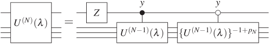
Figure 1: The schematic diagram describing the recursion relation (4aq) of $\hat{U}^{(N)}(\lambda)$. The uppermost line indicates the $N$-th qubit, which plays a role of the control qubit of the controlled unitary operations. When the control qubit is one (zero) the unitary operation connected to the filled (open) circle is applied to the rest of the qubits. $y$ above the circles indicates that the axis of the control-bit is given in the $y$-direction (see  (4ao), the definition of $\hat{C}^{y}_{p}[U]$). In the following, $y$ in circuit diagrams is omitted.

We now solve the eigenvalue problem of $\hat{U}^{(N)}(\lambda)$ recursively. Let $|{}n_{N},\cdots,n_{1};\lambda{}\rangle$ and $\theta^{(N)}(n_{N},\cdots,n_{1};\lambda)$ denote an eigenvector and the corresponding eigenangle of $\hat{U}^{(N)}(\lambda)$, i.e.,

$$\hat{U}^{(N)}(\lambda)|{}n_{N},\cdots,n_{1};\lambda{}\rangle=\rme^{\rmi\theta^{(N)}(n_{N},\cdots,n_{1};\lambda)}|{}n_{N},\cdots,n_{1};\lambda{}\rangle,$$ (4ar)

where $n_{j}\in\left\{0,1\right\}$. We have already solved the case $N=1$ in Section 2 (see (3), (4a) and (4b)): $|{}n_{1};\lambda{}\rangle=|{}n_{1}(\lambda,p_{1}){}\rangle$ and $\theta^{(1)}(n_{1};\lambda)=\theta({n_{1}};\lambda,p_{1})$. For $N>1$, we obtain recursion relations for eigenangles and eigenvectors. Suppose we have an eigenvector $|{}\Psi^{(N-1)}(\lambda){}\rangle$ and the corresponding eigenangle $\Theta^{(N-1)}(\lambda)$ of $\hat{U}^{(N-1)}(\lambda)$. Recall that we obtain $\hat{U}^{(N)}(\lambda)$ by extending $\hat{U}^{(N-1)}(\lambda)$ so as to incorporate one more qubit into it. Let $|{}\phi{}\rangle$ denote a state vector for the qubit newly added to the quantum circuit described by $\hat{U}^{(N-1)}(\lambda)$. A natural candidate of an eigenvector of $\hat{U}^{(N)}(\lambda)$ is $|{}\phi{}\rangle\otimes|{}\Psi^{(N-1)}(\lambda){}\rangle$ because we have

$$\hat{U}^{(N)}(\lambda)\left(|{}\phi{}\rangle\otimes|{}\Psi^{(N-1)}(\lambda){}\rangle\right)=\left[\hat{u}(\lambda^{\prime};p_{N})|{}\phi{}\rangle\right]\otimes|{}\Psi^{(N-1)}(\lambda){}\rangle,$$ (4as)

where $\lambda^{\prime}\equiv\Theta^{(N-1)}(\lambda)$. Accordingly, $|{}n_{N}(\lambda^{\prime},p_{N}){}\rangle\otimes|{}\Psi^{(N-1)}(\lambda){}\rangle$ and $\theta(n_{N};\lambda^{\prime},p_{N})$ with $n_{N}\in\left\{0,1\right\}$ are an eigenvector and the corresponding eigenangle of $\hat{U}^{(N)}(\lambda)$, respectively. This implies the recursion relations

$$\theta^{(N)}(n_{N},\dots,n_{1};\lambda)=\theta(n_{N};\theta^{(N-1)}(n_{N-1},\dots,n_{1};\lambda),p_{N})$$ (4at)

and

$$|{}n_{N},\dots,n_{1};\lambda{}\rangle=|{}n_{N}(\theta^{(N-1)}(n_{N-1},\dots,n_{1};\lambda)){}\rangle\otimes|{}n_{N-1},\dots,n_{1};\lambda{}\rangle,$$ (4au)

for $N>1$.

Assume that the solution of (4at) takes the following form:

$$\theta^{(N)}(n_{N},\dots,n_{1};\lambda)=\frac{2\pi}{2^{N}}\left(m_{N}(n_{N},\dots,n_{1})+d_{N}\frac{\lambda}{2\pi}\right).$$ (4av)

A normalized slope $d_{N}$ of the eigenangle and a “principal quantum number” $m_{N}(n_{N},\dots,n_{1})$ are defined below. For the sake of brevity, we will sometimes omit the arguments $(n_{N},\dots,n_{1})$ of $m_{N}$, so that $\theta^{(N)}(n_{N},\dots,n_{1};\lambda)$ is written as $\theta^{(N)}(m_{N};\lambda)$. For $N=1$, we have $m_{1}(n_{1})=n_{1}$ and $d_{1}=p_{1}$. For $N>1$, (4at) provides the recursion relations:

$$m_{N}=2^{N-1}n_{N}+p_{N}m_{N-1}\qquad\mbox{and}\qquad d_{N}=p_{N}d_{N-1}.$$ (4aw)

Hence we have

$$m_{N} =2^{N-1}n_{N}+\sum_{j=1}^{N-1}\left(\prod_{k=j+1}^{N}p_{k}\right)2^{j-1}n_{j},$$ (4ax)

$$d_{N} =\prod_{k=1}^{N}p_{k}.$$ (4ay)

The solution of the recursion relation (4au) of the eigenvectors is

$$|{}n_{N},\dots,n_{1};\lambda{}\rangle=\bigotimes_{j=1}^{N}|{}n_{j}(\theta^{(j-1)}(m_{j-1};\lambda),p_{j}){}\rangle.$$ (4az)

We remark on the spectral degeneracy of $\hat{U}^{(N)}(\lambda)$. From (4av) and (4ax), the spectral degeneracy is absent if and only if all $p_{2},\dots,p_{N}$ are odd. Note that the degeneracy condition is independent of $p_{1}$ and $\lambda$. Because we focus on the case that there is no spectral degeneracy along the path $C$, we will assume that $p_{2},\dots,p_{N}$ are odd in the following.

5 Eigenangle anholonomy

We here examine the eigenangle anholonomy of the family of quantum circuits described by $\hat{U}^{(N)}(\lambda)$ (4aq). To achieve this, we keep track of the parametric dependence of the eigenangle $\theta^{(N)}(n_{N},\dots,n_{1};\lambda)$ along the cycle $C$, where $\lambda$ is increased by a period $2\pi$. The parametric change of the eigenangle can be expressed as

$$\theta^{(N)}(n_{N},\dots,n_{1};\lambda+2\pi)=\theta^{(N)}(s^{(N)}(n_{N},\dots,n_{1};C);\lambda)+2\pi r^{(N)}(n_{N},\dots,n_{1};C),$$ (4ba)

where $s^{(N)}(n_{N},\dots,n_{1};C)$ is a collection of $N$ quantum numbers and $r^{(N)}(n_{N},\dots,n_{1};C)$ is an integer. In this section, we explain how $s^{(N)}(n_{N},\dots,n_{1};C)$ and $r^{(N)}(n_{N},\dots,n_{1};C)$ are recursively determined. They completely characterize not only the eigenangle anholonomy but also the eigenspace anholonomy when the eigenangles are not degenerate. The reason is that eigenangles have one-to-one correspondence to the eigenspaces if the spectral degeneracy is absent. On the other hand, because the explicit expressions of these quantities are complicated in general, we postpone obtaining explicit solutions; several examples will be shown in Section 7.

The recursive structure in $\hat{U}^{(N)}(\lambda)$ determines $s^{(N)}(n_{N},\dots,n_{1};C)$ and $r^{(N)}(n_{N},\dots,n_{1};C)$. For brevity, we will omit the argument $C$ in the following. Let $s^{(N)}_{j}(n_{N},\dots,n_{1})$ denote the quantum number of $j$-th qubit in $s^{(N)}(n_{N},\dots,n_{1})$ ($1\leq j\leq N$). We note that $s^{(N)}_{j}(n_{N},\dots,n_{1})$ is either $0$ or $1$. For $j<N$, we obtain

$$s^{(N)}_{j}(n_{N},\dots,n_{1})=s^{(N-1)}_{j}(n_{N-1},\dots,n_{1}),$$ (4bb)

using the recursive structure in $\hat{U}^{(N)}(\lambda)$. Hence, $s^{(N)}(n_{N},\dots,n_{1})$ is determined by $s^{(j)}_{j}(n_{j},\dots,n_{1})$ ($1\leq j\leq N$).

We need to find $s^{(N)}_{N}(n_{N},\dots,n_{1})$ and $r^{(N)}(n_{N},\dots,n_{1})$. For $N=1$, we obtain, from the analysis of the single qubit case in Section 2, $s^{(1)}_{1}(n_{1})=s(n_{1},p_{1})$ and $r^{(1)}(n_{1})=r(n_{1},p_{1})$, where $s(n,p)$ and $r(n,p)$ are defined in (4f). In order to clarify the case of $N>1$, we first examine the change of the principal quantum number $m_{N}$ by an increment of $\lambda$ from $0$ to $2\pi$ using  (4ba) and (4av):

$$m_{N}(s^{(N)}(n_{N},\dots,n_{1}))=m_{N}(n_{N},\dots,n_{1})+d_{N}-2^{N}r^{(N)}(n_{N},\dots,n_{1}).$$ (4bc)

Thus we have

$$s^{(N)}_{N}(n_{N},\dots,n_{1}) =s(n_{N},p_{N}r^{(N-1)}(n_{N-1},\dots,n_{1})),$$ (4bda)

$$r^{(N)}(n_{N},\dots,n_{1}) =r(n_{N},p_{N}r^{(N-1)}(n_{N-1},\dots,n_{1})).$$ (4bdb)

We note that it is generally difficult to write down the explicit expressions of the solution of (4bda) and (4bdb). This problem will be dealt with in Section 7.

For the time being, we suppose that we have the solutions $s^{(N)}(n_{N},\dots,n_{1})$ and $r^{(N)}(n_{N},\dots,n_{1})$ to examine gauge invariants. We also assume that the spectral degeneracies are absent, i.e., $p_{2},\dots,p_{N}$ are odd, as explained in the previous section. The permutation matrix $\mathfrak{S}^{(N)}$ is precisely determined by $s^{(N)}(n_{N},\dots,n_{1})$:

$$\{\mathfrak{S}^{(N)}\}_{(n^{\prime}_{N},\dots,n^{\prime}_{1}),(n_{N},\dots,n_{1})}\equiv\prod_{j=1}^{N}\delta_{n^{\prime}_{j},s^{(N)}_{j}(n_{N},\dots,n_{1})}.$$ (4bdbe)

Note that the correspondence between $(n_{N},\dots,n_{1})$ and $m_{N}(n_{N},\dots,n_{1})$ are one-to-one. When we employ the “$m_{N}$”-representation, instead of the $(n_{N},\dots,n_{1})$ representation, the matrix elements of $\mathfrak{S}^{(N)}$ have simpler forms. Because the change induced by a cycle $C$ is represented by the shift of $m_{N}$ by $d_{N}(\mbox{mod\ }2^{N})$, we have

$$\{\mathfrak{S}^{(N)}\}_{m_{N}^{\prime},m_{N}}=\delta_{m_{N}^{\prime},m_{N}+d_{N}{\rm\ mod\ }2^{N}}.$$ (4bdbf)

When $d_{N}$ is odd, or equivalently when $p_{1}$ is odd (see (4ay)), $m_{N}(\mbox{mod $2^{N}$})$ returns to the initial value only after $2^{N}$ repetitions of evolution along $C$. Hence the permutation matrix $\mathfrak{S}$ describes a cycle. On the other hand, if $d_{N}$ is even, $m_{N}\ ({\rm mod\ }2^{N})$ returns with smaller number of repetitions and the period depends on $d_{N}$.

6 Eigenspace anholonomy

We examine the eigenspace anholonomy for $\hat{U}^{(N)}(\lambda)$ along the adiabatic cycle $C$. We find the holonomy matrix $M^{(N)}(C)$ of $\hat{U}^{(N)}(\lambda)$ and the geometric phase $\gamma(C)$ (4am) for the adiabatic cycle $C$ based upon our gauge theoretic formalism described in Section 3.

For the sake of simplicity, we focus on the case that all $p_{j}$’s are odd in this section, which guarantees that the spectral degeneracy is absent. Each eigenvalue and eigenspace returns to their initial ones only after $2^{N}$ cycles along $C$. In other words, this assumption implies the presence of the one-to-one correspondence between quantum numbers $(n_{N},\dots,n_{1})$ and $m_{N}(n_{N},\dots,n_{1})$. Hence we will often abbreviate $(n_{N},\dots,n_{1})$ as $m_{N}$ in the following. Also, for the sake of brevity, we will drop the index $C$.

As shown in Section 3, $M^{(N)}$ can be decomposed into a product of the permutation matrix $\mathfrak{S}^{(N)}$ and a diagonal unitary matrix, i.e.,

$$\{M^{(N)}\}_{m^{\prime}_{N},m_{N}}=\{\mathfrak{S}^{(N)}\}_{m^{\prime}_{N},m_{N}}\sigma^{(N)}(m_{N}),$$ (4bdbg)

where $\sigma^{(N)}(m_{N})$ is a unimodular complex number. Because $\mathfrak{S}^{(N)}$ has been already obtained in the previous section, our task here is to determine the phase factor $\sigma^{(N)}(m_{N})$.

Let us obtain a recursion relation of $M^{(N)}$ ((4bdbq) below) using the gauge connections. The eigenvectors of $\hat{U}^{N}(\lambda)$ form a non-Abelian gauge connection

$$\{A^{(N)}(\lambda)\}_{m^{\prime}_{N},m_{N}} \equiv\langle{}m_{N}^{\prime};\lambda{}|\left[\rmi\partial_{\lambda}|{}m_{N};\lambda{}\rangle\right],$$ (4bdbh)

and the diagonal connection $\{A^{{\rm D}(N)}(\lambda)\}_{m^{\prime}_{N},m_{N}}\equiv\delta_{m^{\prime}_{N},m_{N}}\{A^{(N)}(\lambda)\}_{m^{\prime}_{N},m_{N}},$ which are $2^{N}\times 2^{N}$ Hermite matrices. We now obtain a recursion relation for $A^{(N)}(\lambda)$. For $N=1$, (4a), (4b) and the definition of the gauge connection imply

$$A^{(1)}(\lambda)=\frac{2-p}{4}Y,\quad\mbox{and}\quad A^{\mathrm{D}(1)}(\lambda)=0.$$ (4bdbi)

Namely, for $N=1$, each eigenvector satisfies the parallel transport condition within each eigenspace. For $N>1$, the Leibniz rule suggests a decomposition $A^{(N)}(\lambda)=A_{\rm H}^{(N)}(\lambda)+A_{\rm L}^{(N)}(\lambda)$, where

$$\{A_{\rm H}^{(N)}(\lambda)\}_{m^{\prime}_{N},m_{N}} \equiv\left\{A(\Theta^{\prime}(\lambda),p_{N})\right\}_{n_{N}^{\prime},n_{N}}\partial_{\lambda}\Theta^{\prime}(\lambda)\delta_{m^{\prime}_{N-1},m_{N-1}}$$ (4bdbj)

$$\{A_{\rm L}^{(N)}(\lambda)\}_{m^{\prime}_{N},m_{N}} \equiv\langle{}n_{N}^{\prime}(\Theta^{\prime}(\lambda),p_{N}){}|{}n_{N}(\Theta(\lambda),p_{N}){}\rangle\left\{A^{(N-1)}(\lambda)\right\}_{m^{\prime}_{N-1},m_{N-1}}.$$ (4bdbk)

Here $\Theta(\lambda)\equiv\theta^{(N-1)}(m_{N-1};\lambda)$ and $\Theta^{\prime}(\lambda)\equiv\theta^{(N-1)}(m_{N-1}^{\prime};\lambda)$ are introduced for abbreviations. We also have a similar recursion relation for “diagonal” gauge connection $A^{{\rm D}(N)}(\lambda)$. Because we have chosen the gauge $A^{{\rm D}(N)}(\lambda)=0$ for $N=1$ (see, (4bdbi)), it is straightforward to obtain $A^{{\rm D}(N)}(\lambda)=0$ for an arbitrary $N$ from the recursion relations.

We obtain an explicit expression of $A_{\rm H}^{(N)}(\lambda)$ from the eigenangle of $N$-qubit system (4av) and the gauge connection of the single-qubit system (4bdbi):

$$A_{\rm H}^{(N)}(\lambda) =\frac{(2-p_{N})d_{N-1}}{2^{N+1}}Y\otimes 1^{(N-1)}.$$ (4bdbl)

Next we examine $A_{\rm L}^{(N)}(\lambda)$ in our model. From (4a), (4b) and (4bdbk), we obtain

$$A_{\rm L}^{(N)}(\lambda)=\frac{1+Y}{2}\otimes A_{+}^{(N-1)}(\lambda)+\frac{1-Y}{2}\otimes A_{-}^{(N-1)}(\lambda),$$ (4bdbm)

where

$$A_{\pm}^{(N)}(\lambda) =\rme^{\pm\rmi\pi(2-p_{N+1})2^{-N-1}J_{\rm D}^{(N)}}A^{(N)}(\lambda)\;\rme^{\mp\rmi\pi(2-p_{N+1})2^{-N-1}J_{\rm D}^{(N)}},$$ (4bdbn)

and

$$\left\{J_{\rm D}^{(N)}\right\}_{m^{\prime}_{N},m_{N}}\equiv m_{N}\delta_{m^{\prime}_{N},m_{N}}.$$ (4bdbo)

Accordingly we have

$$A_{\rm L}^{(N)}(\lambda) =\rme^{\rmi{\pi(2-p_{N})}{2^{-N}}Y\otimes J_{\rm D}^{(N-1)}}\left\{1\otimes A^{(N-1)}(\lambda)\right\}\rme^{-\rmi{\pi(2-p_{N})}{2^{-N}}Y\otimes J_{\rm D}^{(N-1)}}.$$ (4bdbp)

Now it is straightforward to prove that $A_{\mathrm{L}}^{(N)}(\lambda)$ and $A^{(N)}(\lambda)$ are independent of $\lambda$. First, we assume the independence of $A^{(N-1)}(\lambda)$ from $\lambda$ for $N>1$. This assumption implies that the $A_{\mathrm{L}}^{(N)}(\lambda)$ is also independent of $\lambda$, from (4bdbp). Because $A_{\mathrm{H}}^{(N)}(\lambda)$ (4bdbl) is also independent of $\lambda$, we conclude the independence of $A^{(N)}(\lambda)$ from $\lambda$. Second, $A^{(1)}(\lambda)$ is independent of $\lambda$ (see, (4bdbi)). Hence we conclude $A_{\mathrm{L}}^{(N)}(\lambda)$ and $A^{(N)}(\lambda)$ for $N\geq 1$ are independent of $\lambda$.

In addition, it is straightforward to see $[A_{\rm H}^{(N)}(\lambda),A_{\rm L}^{(N)}(\lambda)]=0$. Hence the anti-path ordered product is simplified as $M^{(N)}=\rme^{-\rmi 2\pi A_{\rm H}^{(N)}(\lambda)}\rme^{-\rmi 2\pi A_{\rm L}^{(N)}(\lambda)}.$ This implies a recursion relation for the holonomy matrices:

$$M^{(N)} =\frac{1+Y}{2}\otimes\left(\rme^{\rmi{\pi(2-p_{N})}{2^{-N}}J_{\rm D}^{(N-1)}}M^{(N-1)}\rme^{-\rmi{\pi(2-p_{N})}{2^{-N}}(J_{\rm D}^{(N-1)}+d_{N-1})}\right)$$ (4bdbq)

$$\quad{}+\frac{1-Y}{2}\otimes\left(\rme^{-\rmi{\pi(2-p_{N})}{2^{-N}}J_{\rm D}^{(N-1)}}M^{(N-1)}\rme^{\rmi{\pi(2-p_{N})}{2^{-N}}(J_{\rm D}^{(N-1)}+d_{N-1})}\right).$$

From this recursion relation, we obtain the recursion relation for the matrix element of $M^{(N)}$

$$\left\{M^{(N)}\right\}_{m^{\prime}_{N},m_{N}} =\delta_{n_{N}^{\prime},s(n_{N},p_{N}r^{(N-1)})}(-1)^{r(n_{N},p_{N}r^{(N-1)})}\left\{M^{(N-1)}\right\}_{m^{\prime}_{N-1},m_{N-1}},$$ (4bdbr)

which is shown in A.

We now obtain $\sigma^{(N)}(m_{N})$, which is a constituent of $M^{(N)}$ (see (4bdbg)). For $N=1$. it is easy to see $\sigma^{(1)}(n_{1})=(-1)^{r(n_{1},p_{1})}$. From (4bdbr), we find

$$\left\{M^{(N)}\right\}_{m^{\prime}_{N},m_{N}}=\{\mathfrak{S}^{(N)}\}_{m^{\prime}_{N},m_{N}}(-1)^{r^{(N)}}\sigma^{(N-1)}(m_{N-1}),$$ (4bdbs)

which implies a recursion relation for $\sigma^{(N)}$:

$$\sigma^{(N)}(m_{N})=(-1)^{r^{(N)}(m_{N})}\sigma^{(N-1)}(m_{N-1}).$$ (4bdbt)

Hence we have

$$\sigma^{(N)}(n_{N},\dots,n_{1})=(-1)^{\sum_{k=1}^{N}r^{(k)}(n_{k},\dots,n_{1})},$$ (4bdbu)

where we set $r^{(1)}(n_{1})\equiv r(n_{1},p_{1})$. Note that an explicit expression of $r^{(k)}(n_{k},\dots,n_{1})$ depends on $p_{j}$’s.

We examine Manini-Pistolesi’s gauge invariant $\gamma^{(N)}$. From (4ah), we obtain

$$\rme^{\rmi\gamma^{(N)}}=\prod_{n_{N}=0}^{1}\cdots\prod_{n_{1}=0}^{1}\sigma^{(N)}(n_{N},\dots,n_{1}).$$ (4bdbv)

In particular, we have already obtained $\rme^{\rmi\gamma^{(N)}}=-1$ for $N=1$. For $N>1$, (4bdbt) implies $\prod_{n_{N}=0}^{1}\sigma^{(N)}(n_{N},\dots,n_{1})=\prod_{n_{N}=0}^{1}(-1)^{r^{(N)}(n_{N},\dots,n_{1})}$ due to $\left\{\sigma^{(N-1)}(n_{N-1},\dots,n_{1})\right\}^{2}=1$. Thus we have

$$\rme^{\rmi\gamma^{(N)}} =(-1)^{\nu^{(N)}},$$ (4bdbw)

where

$$\nu^{(N)}\equiv\sum_{n_{N}=0}^{1}\cdots\sum_{n_{1}=0}^{1}r^{(N)}(n_{N},\dots,n_{1}).$$ (4bdbx)

Recall that $\nu^{(1)}_{1}=p_{1}$ for $N=1$. From (4bdb), we find $\sum_{n_{N}=0}^{1}r^{(N)}(n_{N},\dots,n_{1})=p_{N}r^{(N-1)}(n_{N-1},\dots,n_{1})$ for $N>1$, because $[j/2]+[(1+j)/2]=j$ holds for an arbitrary integer $j$. It leads us to a recursion relation $\nu^{(N)}=p_{N}\nu^{(N-1)}$, whose solution is

$$\nu^{(N)} =d_{N}.$$ (4bdby)

Since we consider the case that no spectral degeneracy exists implying $d_{N}$ is odd, we find

$$\rme^{\rmi\gamma^{(N)}}=-1$$ (4bdbz)

for $N>0$.

7 Examples

We examine several examples in this section. To complete the characterization of the eigenangle and eigenspace anholonomies of $\hat{U}^{(N)}(\lambda)$, we need to obtain the explicit expressions of $s^{(N)}(n_{N},\dots,n_{1})$ and $r^{(N)}(n_{N},\dots,n_{1})$, as explained in Section 5. This requires to solve (4bda) and (4bdb), whose solution precisely depends on the set of integer parameters $\left\{p_{j}\right\}_{j=1}^{N}$. First, we consider the simplest case $p_{j}=1$ for all $j$. Because we obtain the subsequent cases through the modifications of the simplest one, the study of the first case offers the basis of the following analysis. Second, we replace $p_{1}$ of the simplest case with an even integer. It is shown that the permutation matrix $\mathfrak{S}^{(N)}(C)$ of the second case consists of two cycles. Third, we replace $p_{J}$ in the simplest case with an odd integer. These examples indicates that there are various types of $\mathfrak{S}^{(N)}(C)$ associated with the choices of $\left\{p_{j}\right\}_{j=1}^{N}$.

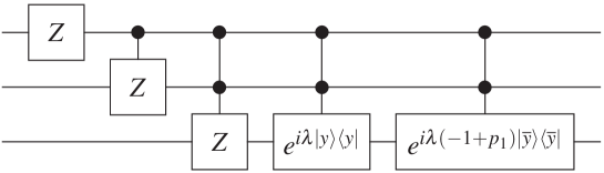
Figure 2: The quantum circuit $\hat{U}^{(3)}(\lambda)$ for three qubits with $p_{2}=p_{3}=1$. $|{}\overline{y}{}\rangle$ is orthogonal to $|{}y{}\rangle$ and normalized. We examine the cases $p_{1}=1$ and $2$ in § 7.1 and § 7.2, respectively. The first examples shown in § 7.3 correspond to the case $p_{1}=3$. The convention for the controlled qubit is explained in the caption of figure 1.

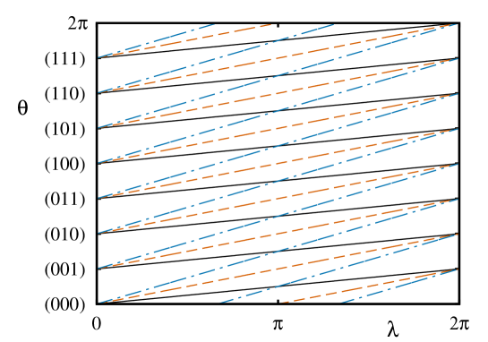
Figure 3: The eigenangles $\theta^{(3)}(n_{3},n_{2},n_{1};\lambda)$ (4av) of $\hat{U}^{(3)}(\lambda)$ with $p_{2}=p_{3}=1$ (see figure 2). The labels of the vertical axis indicate the quantum numbers $(n_{3},n_{2},n_{1})$ of the eigenstates at $\lambda=0$. Three families of lines correspond to $p_{1}=1$ (bold), $p_{1}=2$ (dashed) and $p_{1}=3$ (dash-dotted). Note that $p_{1}$ determines the slope of $\theta^{(3)}(n_{3},n_{2},n_{1};\lambda)$ . Hence different $p_{1}$ induces different itineraries of quantum numbers along adiabatic cycles. In § 7.1, we examine the simplest case $p_{1}=1$. When $p_{1}$ is an even integer, $\mathfrak{S}(C)$ is decomposed into multiple cycles (see (4bdcbcecf) and (4bdcbcecg) in § 7.2). On the other hand, odd $p_{1}$ ensures that $\mathfrak{S}(C)$ describes a cycle (see (4bdcbcecico) in § 7.3, where $p_{1}=3$ is assumed).

7.1 $p_{j}=1$ for all $j$: the simplest case

We here examine the simplest case of $p_{j}=1$ for all $j$ (see figures 2 and 3), which can be reduced to a quantum map under rank-$1$ perturbation [7, 8]. From (4ax), we have

$$m_{N}(n_{N},\dots,n_{1}) =\sum_{j=1}^{N}2^{j-1}n_{j},$$ (4bdca)

which means that $n_{N},\dots,n_{1}$ form coefficients of the binary expansion of the principal quantum number $m_{N}$. This provides a direct relation between $m_{N}$ and $(n_{N},\dots,n_{1})$. It is straightforward to solve (4bda) and (4bdb):

$$s^{(N)}_{N}(n_{N},\dots,n_{1}) =\cases{\overline{n_{N}}&\mbox{for $n_{N-1}\cdots n_{1}=1$}\\ n_{N}&\mbox{otherwise}\\ }$$ (4bdcba)

$$r^{(N)}_{N}(n_{N},\dots,n_{1}) =n_{N}\cdots n_{1},$$ (4bdcbb)

where we define the product of quantum numbers as

$$n_{k}\cdots n_{j} =\cases{\prod_{l=j}^{k}n_{l}&\mbox{for $k\geq j$}\\ 1&\mbox{otherwise}\\ },$$ (4bdcbcc)

throughout this paper.

The principal quantum number $m_{N}$ increases by one after parametric evolution along $C$ once due to $d_{N}=1$: $m_{N}=0\mapsto 1\mapsto\dots 2^{N-1}-1\mapsto 0\mapsto\dots$, whose period is $2^{N}$. On the other hand, the itinerary of $n_{N},\dots,n_{1}$ of $N=3$, for example, is

$$000\mapsto 001\mapsto 010\mapsto 011\mapsto 100\mapsto 101\mapsto 110\mapsto 111\mapsto 000\mapsto\dots.$$

7.2 The simplest case perturbed with $p_{1}\neq 1$: $p_{1}$ is even

We examine the case of $p_{j}=1$ for $j>1$ and $p_{1}$ is an even integer, which corresponds to the simplest case perturbed with a certain even $p_{1}\neq 1$ (see figures 2 and 3). Note that the mapping between $n_{N},\dots,n_{1}$ and $m_{N}$ is independent of $p_{1}$, while the spectrum depends on $p_{1}$:

$$\theta^{(N)}(n_{N},\dots,n_{1}) =\frac{2\pi}{2^{N}}\left(m_{N}(n_{N},\dots,n_{1})+p_{1}\frac{\lambda}{2\pi}\right).$$ (4bdcbcd)

Hence as $\lambda$ increases by every $2\pi$, the principal quantum number $m_{N}$ also increases by $p_{1}$. It means that $m_{N}{\rm\ mod\ }2^{N}$ returns to the initial point after $2^{N-1}$ cycles of $C$. Furthermore, a suitable choice of $p_{1}$ make the period even shorter. This is the crucial difference from the case that $p_{1}$ is odd, as discussed later.

For the sake of simplicity, we assume $p_{1}=2$ so as to find the explicit expressions of $s^{(N)}$ and $r^{(N)}$. For $N=1$, we have $s^{(1)}_{1}(n_{1})=n_{1}$, $r^{(1)}(n_{1})=1$. For $N\geq 2$, one finds

$$s^{(N)}_{N}(n_{N},\dots,n_{1}) =\cases{\overline{n_{N}}&\mbox{for $n_{N-1}\cdots n_{2}=1$}\\ n_{N}&\mbox{otherwise}\\ },$$ (4bdcbcea)

$$r^{(N)}_{N}(n_{N},\dots,n_{1}) =n_{N}\cdots n_{2}.$$ (4bdcbceb)

Hence the first qubit is decoupled from others. The rest of the qubits are equivalent to the simplest case with $N-1$ qubits.

For $p_{1}=2$, the permutation matrix $\mathfrak{S}^{(N)}(C)$ forms two sorts of cycles consisting of even or odd $m_{N}$’s. For $N=3$, the case of even $m_{N}$ reads

$$000\mapsto 010\mapsto 100\mapsto 110\mapsto 000\mapsto\dots,$$ (4bdcbcecf)

while for odd $m_{N}$’s

$$001\mapsto 011\mapsto 101\mapsto 111\mapsto 001\mapsto\dots.$$ (4bdcbcecg)

We remark that $n_{1}$ remains unchanged along these itineraries. Namely, the initial qubit is repeatedly recovered during the evolution.

7.3 The simplest case perturbed with odd $p_{J}$

Here we consider the case that $p_{j}=p\delta_{jJ}+(1-\delta_{jJ})$, where $J$ is an integer ($0<J\leq N$) and $p=1+2^{K}$ ($K$ is a positive integer). In other words, we obtain this model by replacing $p_{J}$ of the simplest case, where we set $p_{j}=1$ for all $j$, with $p$. We examine how such a tiny change affect the eigenangle and eigenspace anholonomies. When this new model consists of smaller number qubits, i.e., $N<J$, it becomes equivalent to the simplest model. The effect of the replacement of $p_{J}$ appears only when the system size is large, i.e., $N\geq J$.

First, we note that

$$m_{N}(n_{N},\dots,n_{1})=\sum_{j=1}^{N}2^{j-1}n_{j}+\sum_{j=1}^{J-1}2^{K+j-1}n_{j},$$ (4bdcbcech)

where the second term in the rhs is defined as $0$ if $J=1$. We also note that the spectral degeneracy is absent since $p$ is odd

We show explicit expressions of $s_{N}^{(N)}(n_{N},\dots,n_{1})$ and $r^{(N)}(n_{N},\dots,n_{1})$, which govern the anholonomy in the quantum number. Because this model agrees with the simplest case for $N<J$, $s^{(N)}_{N}(n_{N},\dots,n_{1})$ and $r^{(N)}_{N}(n_{N},\dots,n_{1})$ satisfy (4bdcba) and (4bdcbb) for $N<J$. The effect of the $p_{J}\neq 1$, which we may call an “impurity” of the simplest model, sets in at $N=J$. For $J\leq N<J+K$, one finds

$$s^{(N)}_{N}(n_{N},\dots,n_{1}) =\cases{\overline{n_{N}}&\mbox{for $n_{N-1}\cdots n_{1}=1$}\\ n_{N}&\mbox{otherwise}\\ },$$ (4bdcbcecia)

$$r^{(N)}(n_{N},\dots,n_{1}) =(n_{N}\cdots n_{J}+2^{K-(N-J)-1})n_{J-1}\cdots n_{1}.$$ (4bdcbcecib)

Hence the effect of the impurity $p_{J}$ on $r^{(N)}$ is largest at $N=J$, and becomes smaller as $N$ increases for $J\leq N<J+K$. In other words, $r^{(N)}$’s of $K$ qubits are directly affected by the impurity. The $J+K$-th qubit is in another regime:

$$s^{(J+K)}_{J+K}(n_{J+K},\dots,n_{1})=\cases{\overline{n_{J+K}}&\mbox{for $n_{J+K-1}\cdots n_{J}=0$ and $n_{J-1}\dots n_{1}=1$}\\ n_{J+K}&\mbox{otherwise}}.$$ (4bdcbcecicj)

The influence of the qubit with index $j$ ($j=J,\dots,J+K$) on the qubits with larger index can be described through a quantum number

$$t^{(J,K)}(n_{J+K},\dots,n_{J})\equiv n_{J+K}+\overline{n_{J+K}}n_{J+K-1}\cdots n_{J},$$ (4bdcbcecick)

which is either $0$ or $1$. It seems that the impurity introduces an effective $(K+1)$-body interaction among the quantum numbers $(n_{J+K},\dots,n_{J})$. This determines $r^{(N)}$ for $N\geq J+K$ as

$$r^{(N)}(n_{N},\dots,n_{1})=n_{N}\dots n_{J+K+1}t^{(J,K)}n_{J-1}\cdots n_{1},$$ (4bdcbcecicl)

where we omit the argument of $t^{(J,K)}(n_{J+K},\dots,n_{J})$. On the other hand, for $N>J+K$, we have

$$s^{(N)}_{N}(n_{N},\dots,n_{1}) =\cases{\overline{n_{N}}&\mbox{for $n_{N-1}\cdots n_{J+K+1}t^{(J,K)}n_{J-1}\cdots n_{1}=1$}\\ n_{N}&\mbox{otherwise}}.$$ (4bdcbcecicm)

We consider two typical cases. The first example is the case of $J=1$ and $K=1$ (see figures 2 and 3), where the principal quantum number $m_{N}$ is unaffected by the impurity due to $J=1$ (see, (4bdcbcech)). As shown above, a cycle $C$ corresponds to the increment of $m_{N}$ by $d_{N}=p_{1}=3$. For example, with $N=3$, we have

$$0\mapsto 3\mapsto 6\mapsto 1\mapsto 4\mapsto 7\mapsto 2\mapsto 5\mapsto 0\mapsto\dots.$$ (4bdcbcecicn)

In terms of $n_{j}$s, the itinerary is

$$000\mapsto 011\mapsto 110\mapsto 001\mapsto 100\mapsto 111\mapsto 010\mapsto 101\mapsto 000\mapsto\dots.$$ (4bdcbcecico)

This itinerary can be understood through the simple correspondence between $n_{N},\dots,n_{1}$ and $m_{N}$, as shown in (4bdcbcech). Namely, $n_{N},\dots,n_{1}$ are coefficients of the binary expansion of $m_{N}$.

The second example is the case of $J=2$ and $K=1$ (see figure 4 and 5), where the effect of $p_{J}\neq 1$ appears not only in the eigenangle but also in $m_{N}(n_{N},\dots,n_{1})$ (see, (4bdcbcech)). On the other hand, the itinerary of $m_{N}$ induced by the repetition of the cycle $C$ remains intact to be equivalent to the case $J=1$ and $K=1$ discussed above; i.e., a cycle $C$ corresponds to the increment of $m_{N}$ by $3$. We depict the itinerary of quantum numbers $n_{j}$ induced by the cycle $C$. For $N=3$, we have $m_{3}=4n_{3}+2n_{2}+3n_{1}$ and

$$000\mapsto 001\mapsto 110\mapsto 111\mapsto 100\mapsto 101\mapsto 010\mapsto 011\mapsto 000\mapsto\dots.$$ (4bdcbcecicp)

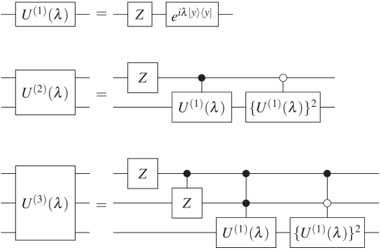
Figure 4: The quantum circuits $\hat{U}^{(N)}(\lambda)$ ($N=1,2$, and $3$) with $p_{1}=p_{3}=1$ and $p_{2}=3$. The cases of $N=2$ and $3$ are rather complicated due to the recursive structure with $p_{2}\neq 1$. This is the second example shown in § 7.3. The convention for the controlled qubit is explained in the caption of figure 1.

Figure 5: The eigenangles $\theta^{(3)}(n_{3},n_{2},n_{1};\lambda)$ (4av) of $\hat{U}^{(3)}(\lambda)$ depicted in figure 4. The labels of the vertical axis indicate the quantum numbers $(n_{3},n_{2},n_{1})$ of the eigenstates at $\lambda=0$. The order of the quantum numbers at the initial point $\lambda=0$ is different from that of figure 3. Namely the initial quantum numbers are scrambled by $p_{2}\neq 1$. The corresponding itinerary of quantum numbers is shown in (4bdcbcecicp).

8 Complexity of the anholonomy

The repetition of the adiabatic cycle $C$ in $\hat{U}^{(N)}(\lambda)$ generates an itinerary of the quantum numbers $(n_{N},\dots,n_{1})$. We point out that the itinerary involves an NP-complete problem in this section.

The examples in the previous sections tells us that the expressions of $s^{(N)}_{N}$’s and $r^{(N)}$’s are rather simple when $p_{j}=1$ for all $j$. In contrast, when we make any $p_{j}$ different from $1$, the expressions of $s^{(N)}_{N}$’s and $r^{(N)}$’s become slightly complicated. One may expect that the more $p_{j}$’s differ from 1, the more complicated they become, so does the itinerary of $(n_{N},\dots,n_{1})$ induced by the adiabatic cycle $C$. However, this is not true because the itinerary of $m_{N}$ remains simple irrespective of variation of $p_{j}$’s; $m_{N}$ increases only by $d_{N}$ for a cycle $C$. How do we justify this? We will show that the cost to obtain $n_{N}\dots n_{1}$ for a given $m_{N}$ is generally equivalent to that of finding the solution of the subset-sum problem, which is a NP-complete problem. We also explain the relationship between their equivalence and the adiabatic quantum computation [13] along an eigenangle [14]. For the sake of simplicity, we focus on the case that all $p_{j}$ is odd. Then, the spectral degeneracy is absent, and the shortest period of the itinerary is $2^{N}$ in the unit of the cycle $C$.

First, we explain our task to find $(n_{N}\dots n_{1})$ for a given $m_{N}$. From (4ax), this is to solve the following equation

$$m_{N} =\sum_{j=1}^{N}w_{j}n_{j},$$ (4bdcbcecicq)

where

$$w_{j}\equiv\left(\prod_{k=j+1}^{N}p_{k}\right)2^{j-1}$$ (4bdcbcecicr)

for $1\leq j<N$, and $w_{N}\equiv 2^{N-1}$.

Second, we explain the subset-sum problem [22]. A subset-sum problem has two parameters $S$ and $t$. $S$ is a finite set of positive integers. $t$ is a positive integer, and is called a target. The problem is to show whether there exists a set $S^{\prime}\subseteq S$ such that $t=\sum_{s\in S^{\prime}}s$. For our purpose, we need to obtain $S^{\prime}$.

Now we explain the equivalence between our problem and the subset-sum. In our case, let $S$ be $\left\{w_{j}\right\}_{j=1}^{N}$, which is a set of positive integers. Finding $(n_{N}\dots n_{1})$ that satisfy (4bdcbcecicq) is essentially equivalent to the problem to find a set of positive integers $S^{\prime}\subseteq S$ such that $m_{N}=\sum_{s\in S^{\prime}}s$. This justifies the equivalence.

This explanation has a subtle point. During a course of the repetition of the cycle $C$, $m_{N}$ can be determined only up to modulo $2^{N}$. However, this does not break the equivalence in the difficulty of the solving the problems

Based upon this equivalence, we examine whether the evolution along the adiabatic increment of $\lambda$ in $\hat{U}^{(N)}(\lambda)$ offers an efficient way to solve the subset-sum problem. It turns out that the adiabatic approach is inefficient. First, when $\lambda$ is varied slow enough, we can prepare $m_{N}$ to be an arbitrary positive integer. Next, appropriate measurements of qubits ascertain $n_{N},\dots,n_{1}$. To make the nonadiabatic error small enough, there is a lower bound of the running time for quantum evolution. This is essentially determined by the gap $\Delta$ between the eigenangles. From the exact expression of the eigenangle (4av), we obtain $\Delta\propto 2^{-N}$ for large $N$. Hence the lower bound of the running time must be exponentially large, i.e., the adiabatic approach is inefficient.

We remark on the inefficiency to obtain $\hat{U}^{(N)}(\lambda)$ from quantum gates. Our construction described in (4aq), of $\hat{U}^{(N)}(\lambda)$ is generally inefficient, because (4aq) requires exponentially many quantum gates for general $\left\{p_{j}\right\}_{j=0}^{\infty}$. On the other hand, if we impose $p_{j}=1$ for most $j$ except for infinitely many $j$, the number of quantum gates required to construct $\hat{U}^{(N)}(\lambda)$ can be a polynomial of $N$. However, we are not certain whether such a $\hat{U}^{(N)}(\lambda)$ involves any NP-complete problem.

9 Discussion

We here discuss the relationship between our result and the recent work on the topological characterization of periodically driven systems [15]. The work in [15] offers an integer

$$\nu(C)\equiv\frac{1}{2\pi\rmi}\oint_{C}\mathop{\mathrm{Tr}}\nolimits[\{\hat{U}(\lambda)\}^{-1}\partial_{\lambda}\hat{U}(\lambda)]\rmd\lambda,$$ (4bdcbcecics)

for a family of Floquet operator $\hat{U}(\lambda)$ in a closed path $C$ in the parameter space of $\lambda$. Because $\nu(C)$ can be regarded as a gauge invariant for the adiabatic cycle $C$, it is worth comparing it with our gauge invariants $\mathfrak{S}(C)$ and $\gamma(C)$.

First, we show that $\nu(C)$ is indeed an integer. Let $\hat{U}(\lambda)$ denote a Floquet operator of a periodically driven system. We assume that $\hat{U}(\lambda)$ is periodic in $\lambda$ and its shortest period is $2\pi$, which guarantees its spectrum $\left\{\rme^{\rmi\theta_{n}(\lambda)}\right\}_{n=0}^{N-1}$ is also periodic in $\lambda$, where $N$ is the dimension of the Hilbert space and $\theta_{n}(\lambda)$ is an eigenangle. Such a spectral periodicity implies

$$\theta_{s(n)}(0)=\theta_{n}(2\pi)+2\pi r(n),$$ (4bdcbcecict)

where $s(n)$ describes a permutation over quantum numbers $\left\{0,\dots,N-1\right\}$, and $r(n)$ is an integer. The latter integer has an integral expression

$$2\pi r(n)=\int_{0}^{2\pi}\frac{\partial\theta_{n}(\lambda)}{\partial\lambda}\rmd\lambda.$$ (4bdcbcecicu)

The derivative of eigenangle is $\partial\theta_{n}(\lambda)/\partial\lambda=-\rmi\langle{}n(\lambda){}|\{\hat{U}(\lambda)\}^{-1}\{\partial_{\lambda}\hat{U}(\lambda)\}|{}n(\lambda){}\rangle,$ where $|{}n(\lambda){}\rangle$ is a normalized eigenvector of $\hat{U}(\lambda)$ corresponding to the eigenangle $\theta_{n}(\lambda)$ [23]. Hence we obtain

$$2\pi r(n)=-\rmi\int_{0}^{2\pi}\langle{}n(\lambda){}|\{\hat{U}(\lambda)\}^{-1}\{\partial_{\lambda}\hat{U}(\lambda)\}|{}n(\lambda){}\rangle\rmd\lambda.$$ (4bdcbcecicv)

A sum rule on $2\pi r(n)$ has a representation-independent expression:

$$2\pi\sum_{n=0}^{N-1}r(n)=\frac{1}{\rmi}\int_{0}^{2\pi}\mathop{\mathrm{Tr}}\nolimits\left[\{\hat{U}(\lambda)\}^{-1}\{\partial_{\lambda}\hat{U}(\lambda)\}\right]\rmd\lambda.$$ (4bdcbcecicw)

We remark that this sum rule is the key to prove the presence of the eigenvalue and eigenspace anholonomies in the quantum map under a rank-$1$ perturbation [6, 7]. (4bdcbcecics) and (4bdcbcecicw) imply

$$\nu(C)\equiv\sum_{n=0}^{N-1}r(n),$$ (4bdcbcecicx)

which is an integer. This argument suggests that $\nu(C)$ characterizes the winding of eigenangles, or equivalently, quasienergies.

We now compare $\nu(C)$ with the permutation matrix $\mathfrak{S}(C)$. We examine the classification of a closed path $C$ for a family of the quantum circuit on a qubit, using $\nu(C)$. We recall that $\mathfrak{S}(C)$ is shown to classify $C$ into two classes in Sec. 2. This is obtained by an inspection of $C_{p}$, which corresponds to the family of unitary $\hat{u}(\lambda,p)$ (2) for $0\leq\lambda\leq 2\pi$. In particular, even and odd $p$ correspond to (4p) and (4v), respectively. As for $\nu(C)$, it is straightforward to see $\nu(C_{p})=p$. The stability of the topological quantity $\nu(C)$ against a small deformation of closed path from $C_{p}$ implies that $\nu(C)$ of a closed path $C$ takes an arbitrary integer. Hence $\nu(C)$ classifies the closed paths into an infinitely many classes. Thus $\nu(C)$ exhibits a detailed structure than $\mathfrak{S}(C)$ as for the closed paths for the space of single-qubit quantum circuits.

This conclusion does not hold for the quantum circuits with multiple qubits. To see this, we examine the quantum circuits $\hat{U}^{(N)}(\lambda)$ introduced in Sec. 4. We have already obtained the corresponding integer $\nu^{(N)}(C)$ in (4bdby) to evaluate the geometric phase $\gamma^{(N)}(C)$. The examples shown in Sec. 7.3 tells us that $\mathfrak{S}^{(N)}(C)$ can take various values even for a certain given $\nu^{(N)}(C)$. Thus we conclude that the role of $\mathfrak{S}^{(N)}(C)$ and $\nu^{(N)}(C)$ are independent in classifying the families of quantum circuits.

In order to provide another comparison of $\mathfrak{S}(C)$ and $\nu(C)$, we show an example in which $C$ contains the crossing of eigenvalues. Note that we have excluded such cases so far in this paper. We will show that $\mathfrak{S}(C)$ is sensitive to the eigenvalue crossing, while $\nu(C)$ is not [15]. Let us examine the following quantum circuit

$$\hat{u}_{Y}(\lambda,p)\equiv\rme^{\rmi(p-1)\lambda(1-|{}y{}\rangle\langle{}y{}|)+\rmi\lambda|{}y{}\rangle\langle{}y{}|}\hat{Y},$$ (4bdcbcecicy)

which is obtained by replacing $\hat{Z}$ with $\hat{Y}\equiv 1-2|{}y{}\rangle\langle{}y{}|$ in $\hat{u}(\lambda,p)$ (2). These quantum circuits are periodic in $\lambda$. Let $C_{{Y}}$ denote the closed path in quantum circuits specified by $\hat{u}_{Y}(\lambda,p)$ with $0\leq\lambda\leq 2\pi$. The crucial point is that $C_{{Y}}$ involves an eigenvalue crossing, because the eigenvalues of $\hat{u}_{Y}(\lambda,p)$ degenerate at $\lambda=0$. Also, the eigenvector of $\hat{u}_{Y}(\lambda,p)$ is independent of $\lambda$. Hence $\mathfrak{S}(C_{{Y}})$ is the identity matrix (4p). We explain that $\mathfrak{S}(C)$ in the vicinity of $C=C_{Y}$ is generically different from the identity matrix. Let us introduce another unitary matrix $\hat{Y}^{\prime}$, which satisfies $[\hat{Y}^{\prime},\hat{Y}]\neq 0$. When we replace $\hat{Y}$ in $\hat{u}_{Y}(\lambda,p)$ with $\hat{Y^{\prime}}$, the corresponding family of quantum circuit exhibits the eigenspace and eigenangle anholonomies, according to the analysis in [6]. Hence $\mathfrak{S}(C)$ is the permutation matrix whose cycle is $2$  (4v). This conclusion holds even when the difference between $\hat{Y}$ and $\hat{Y}^{\prime}$ is arbitrary small. Thus, $\mathfrak{S}(C)$ is sensitive to $C$ in the vicinity of $C_{Y}$. In contrast, $\nu(C)=p$ is independent of $\hat{Y}$ in $\hat{u}_{Y}(\lambda,p)$, as long as $\hat{Y}$ is unitary. In this sense, $\nu(C)$ is stable against the choice of $C$, even when $C$ involves the crossing of eigenvalues.

We close this discussion with a comment on the gauge invariants obtained here. All gauge invariants are determined by the integers $s(n;C)$ and $r(n;C)$, which are defined in (4ba) (see also, (4bdcbcecict)), as for the adiabatic cycle $C$ of quantum circuits $\hat{U}^{(N)}(\lambda)$ (4aq). The permutation matrix $\mathfrak{S}^{(N)}$ contains all $s(n)$’s. On the other hand, $\nu(C)$ (4bdcbcecicx) is the whole sum of $r(n)$’s. We find that $\nu(C)$ determines the geometric phase $\gamma(C)$ through (4bdbw). It remains to be clarified whether the intimate relationship between $\nu(C)$ and $\gamma(C)$ holds in general. Also, it is worth to clarify whether other combinations of $r(n)$’s give us any useful insights on the anholonomies.

10 Summary

In this paper, we have identified the gauge invariants $\mathfrak{S}(C)$ and $\gamma(C)$ that are associated with the eigenvalue and eigenspace anholonomies for the closed path $C$ of a family of unitary operators. The unified theory of quantum anholonomy has been revisited to clarify that $\gamma(C)$ is the Berry phase for the $N$-repetition of closed path $C^{N}$, where $N$ is the dimension of the relevant Hilbert space. By using a family of quantum circuits that are recursively constructed, these gauge invariants have been analyzed in detail. It has been shown that a generic family of the quantum circuits is associated with an NP-complete problem. The relationship between our gauge invariants and Kitagawa et al.’s topological integer $\nu(C)$ has been also discussed.

Appendix A A proof of (4bdbr)

We will obtain the recursion relation (4bdbr) of the matrix element of $M^{(N)}$ from the recursion relation (4bdbq) of $M^{(N)}$.

First, to simplify (4bdbq), we need to evaluate $\rme^{\rmi\alpha J_{\rm D}^{(N)}}M^{(N)}\rme^{-\rmi\alpha J_{\rm D}^{(N)}}$. Because $J_{\rm D}^{(N)}$ (4bdbo) is diagonal and $M^{(N)}$ is the product of a permutation and a diagonal unitary matrices (see,  (4bdbg)), we have

$$\left\{[J_{\rm D}^{(N)},M^{(N)}]\right\}_{m^{\prime}_{N},m_{N}}=\{M^{(N)}\}_{m^{\prime}_{N},m_{N}}\left[m_{N}(s^{(N)}(n_{N},\dots,n_{1}))-m_{N}(n_{N},\dots,n_{1})\right].$$ (4bdcbcecicz)

Furthermore, using the recursion relation (4bc) for $m_{N}$, we obtain

$$\left\{[J_{\rm D}^{(N)},M^{(N)}]\right\}_{m^{\prime}_{N},m_{N}}=\{M^{(N)}\}_{m^{\prime}_{N},m_{N}}\left(d_{N}-2^{N}r^{(N)}\right),$$ (4bdcbcecida)

where $r^{(N)}(n_{N},\dots,n_{1})$ is abbreviated as $r^{(N)}$. Now it is straightforward to show

$$\left\{\rme^{\rmi\alpha J_{\rm D}^{(N)}}M^{(N)}\rme^{-\rmi\alpha J_{\rm D}^{(N)}}\right\}_{m^{\prime}_{N},m_{N}}=\left\{M^{(N)}\right\}_{m^{\prime}_{N},m_{N}}\rme^{\rmi\alpha\left(d_{N}-2^{N}r^{(N)}\right)}.$$ (4bdcbcecidb)

Hence, we obtain from  (4bdbq)

$$\left\{M^{(N)}\right\}_{m^{\prime}_{N},m_{N}}=\left\{\rme^{-\rmi(\pi/2)(2-p_{N})r^{(N-1)}Y}\right\}_{n_{N}^{\prime},n_{N}}\left(M^{(N-1)}\right)_{m^{\prime}_{N-1},m_{N-1}}.$$ (4bdcbcecidc)

When $r^{(N-1)}$ is even, the first factor in rhs of  (4bdcbcecidc) is written as

$$\left\{\rme^{-\rmi\pi(2-p_{N})r^{(N-1)}Y/2}\right\}_{n_{N}^{\prime},n_{N}}=\delta_{n_{N}^{\prime},n_{N}}(-1)^{-(2-p_{N})r^{(N-1)}/2}.$$ (4bdcbcecidd)

On the other hand, when $r^{(N-1)}$ is odd, we have

$$\left\{\rme^{-\rmi\pi(2-p_{N})r^{(N-1)}Y/2}\right\}_{n_{N}^{\prime},n_{N}}=\delta_{n_{N}^{\prime},\overline{n_{N}}}(-1)^{n_{N}}(-1)^{[(2-p_{N})r^{(N-1)}(n_{N-1},\dots,n_{1})-1]/2}.$$ (4bdcbcecide)

We then obtain, using the definition of $r(n,p)$ (4f),

$$\left\{\rme^{-\rmi\pi(2-p_{N})r^{(N-1)}Y/2}\right\}_{n_{N}^{\prime},n_{N}}=\delta_{n_{N}^{\prime},s(n_{N},p_{N}r^{(N-1)})}(-1)^{r(n_{N},p_{N}r^{(N-1)})}.$$ (4bdcbcecidf)

Hence (4bdbr) is proved.

References

References

- [1] Berry M V 1984 Proc. R. Soc. London A 392 45
- [2] Cheon T 1998 Phys. Lett. A 248 285
- [3] Albeverio S, Gesztesy F, Hoegh-Krohn R and Holden H with an appendix by Exner P 2005 Solvable Models in Quantum Mechanics 2nd edn (Rhode Island: AMS Chelsea) Appendix K
- [4] Cheon T, Tanaka A and Kim S W 2009 Phys. Lett. A 374 144
- [5] Tanaka A and Cheon T 2010 Phys. Rev. A 82 022104
- [6] Tanaka A and Miyamoto M 2007 Phys. Rev. Lett. 98 160407
- [7] Miyamoto M and Tanaka A 2007 Phys. Rev. A 76 042115
- [8] Tanaka A, Kim S W and Cheon T 2011 Europhys. Lett. 96 10005
- [9] Wilczek F and Zee A 1984 Phys. Rev. Lett. 52 2111
- [10] Cheon T and Tanaka A 2009 Europhys. Lett. 85 20001
- [11] Fujikawa K 2005 Phys. Rev. D 72 025009
- [12] Bohm A, Mostafazadeh A, Koizumi H, Niu Q and Zwanziger Z 2003 The Geometric Phase in Quantum Systems (Berlin: Springer)
- [13] Farhi E, Goldstone J, Gutmann S and Sipser M 2000 Quantum computation by adiabatic evolution Preprint quant-ph/0001106
- [14] Tanaka A and Nemoto K 2010 Phys. Rev. A 81 022320
- [15] Kitagawa T, Berg E, Rudner M and Demler E 2010 Phys. Rev. B 82 235114
- [16] Tanaka A and Cheon T 2009 Ann. Phys. (N.Y.) 324 1340
- [17] Stone A J 1976 Proc. R. Soc. London A 351 141
- [18] Samuel J and Bhandari R 1988 Phys. Rev. Lett. 60 2339
- [19] Manini N and Pistolesi F 2000 Phys. Rev. Lett. 85 3067
- [20] Mead C and Truhlar D G 1979 J. Chem. Phys. 70 2284
- [21] Georgi H 1999 Lie Algebras in Particle Physics 2nd edn (Colorado: Westview press) Chap 1
- [22] Cormen T H et al. 2009 Introduction to Algorithms 3rd edn (Massachusetts: The MIT Press) § 34.5.5.
- [23] Nakamura K and Lakshmanan M 1986 Phys. Rev. Lett. 57 1661