Spacelike pion form factor from analytic continuation and the onset of perturbative QCD

Abstract

The factorization theorem for exclusive processes in perturbative QCD predicts the behavior of the pion electromagnetic form factor $F(t)$ at asymptotic spacelike momenta $t(=-Q^{2})<0$. We address the question of the onset energy using a suitable mathematical framework of analytic continuation, which uses as input the phase of the form factor below the first inelastic threshold, known with great precision through the Fermi-Watson theorem from $\pi\pi$ elastic scattering, and the modulus measured from threshold up to 3 GeV by the BaBar Collaboration. The method leads to almost model-independent upper and lower bounds on the spacelike form factor. Further inclusion of the value of the charge radius and the experimental value at $-2.45\,\text{GeV}^{2}$ measured at JLab considerably increases the strength of the bounds in the region $Q^{2}\lesssim 10\,\text{GeV}^{2}$, excluding the onset of the asymptotic perturbative QCD regime for $Q^{2}<7\,\text{GeV}^{2}$. We also compare the bounds with available experimental data and with several theoretical models proposed for the low and intermediate spacelike region.

I Introduction

The high-energy behavior along the spacelike axis of the pion electromagnetic form factor is predicted by factorization in perturbative QCD [1, 2, 3, 4], which to leading order (LO) gives

$$F^{\rm LO}_{\rm pert}(-Q^{2})=\frac{8\pi f_{\pi}^{2}\alpha_{s}(\mu^{2})}{Q^{2}},$$ (1)

where $f_{\pi}=130.4\,\text{MeV}$ is the pion decay constant and $\alpha_{s}(\mu^{2})$ the strong coupling at the renormalization scale $\mu^{2}$. Next-to-leading-order (NLO) perturbative corrections have been calculated in [5, 6, 7, 8, 9, 10, 11], using various renormalization schemes and pion distribution amplitudes (DAs). In particular, the result in the ${\overline{\rm MS}}$-renormalization scheme with asymptotic DAs reads [10]

$$F^{\rm NLO}_{\rm pert}(-Q^{2})=\frac{8f_{\pi}^{2}\alpha_{s}^{2}(\mu^{2})}{Q^{2}}\,\left[\frac{\beta_{0}}{4}\left(\ln\frac{\mu^{2}}{Q^{2}}+\frac{14}{3}\right)-3.92\right],$$ (2)

where $\beta_{0}=11-2n_{f}/3$ is the first coefficient in the perturbative expansion of the $\beta$-function, $n_{f}$ being the number of active flavors. The ambiguities that affect the perturbative QCD predictions have been investigated in many papers, where, in particular, the dependence on the renormalization scale $\mu^{2}$ and various prescriptions for scale setting have been discussed [12, 10].

It has been known for a long time that in the case of the pion form factor the asymptotic regime sets in quite slowly, due to the complexity of soft, nonperturbative processes in QCD in the intermediate $Q^{2}$ region. Many nonperturbative approaches have been proposed for the study of the form factor, including QCD sum rules [13], quark-hadron local duality [14, 15, 16, 17], extended vector meson dominance [18], light-cone sum rules [19, 20, 21], sum rules with nonlocal condensates [22, 23, 24], and anti-de Sitter (AdS)/QCD models [25, 26]. The scale of the onset in the presence of Sudakov corrections [27] and large $N_{c}$ Regge approaches [28] suggests that it can be very large. However, constructing a fully valid model to describe the form factor at intermediate energies in fundamental QCD still remains a major theoretical challenge.

On the experimental side, several measurements of the spacelike form factor at various energies are available (see Refs. [29, 30, 31, 32, 33, 34, 35, 36, 37, 38, 39]), the most precise being the recent results of the JLab Collaboration [38, 39] with the highest measurement being at $Q^{2}=2.45\,\text{GeV}^{2}$. The experimental determination of $F$ at larger values of $Q^{2}$ is difficult due to the lack of a free pion target and requires the use of pion electroproduction from a nucleon target. This stems from a virtual photon coupling to a pion in the cloud surrounding the nucleon. In this regard, there are uncertainties associated with the off shellness of the struck pion and the consequent extrapolation to the physical pion mass pole, which leads to uncertainties in the extraction of the value of the form factor at $t=0$, and possible contributions from nonresonant backgrounds. The lack of reliable experimental data in the higher $Q^{2}$ region is a major obstacle to confirm or discard the number of theoretical models already available. In particular, it remains an open question as to at what value of $Q^{2}$ do the nonperturbative contributions become negligible so that the perturbative QCD description of the form factor becomes reliable.

In the recent past, the knowledge of the form factor has improved considerably on the timelike axis. The phase of the form factor in the elastic region of the unitarity cut (below the first inelastic threshold associated with the $\pi\omega$ state) is equal, by the final state interaction theorem also known as the Fermi-Watson theorem, to the $P$-wave phase shift of the elastic $\pi\pi$ scattering amplitude, which has been calculated recently with precision using Roy equations [40, 41, 42, 43]. The modulus has been measured from the cross section of $e^{+}e^{-}\to\pi^{+}\pi^{-}$ by several groups in the past, and more recently to high accuracy by BaBar [44] and KLOE [45, 46] Collaborations. In particular, the high statistics measurement by BaBar yields the modulus at high precision up to an energy of 3 GeV. Therefore, an interesting possibility is to find constraints on the spacelike form factor by the analytic extrapolation of the accurate timelike information.

In the present paper we address precisely this problem. Namely, our aim is to perform an analytic continuation of the form factor from the timelike to the spacelike region using in a most conservative way the available information on the phase and modulus on the unitarity cut, and also spacelike information. The main result of the method will consist of rather stringent upper and lower bounds at values of spacelike momenta, which provide a criterion for finding a lower limit for the onset of the QCD perturbative behavior.

We start by briefly discussing, in Sec.II, several methods of analysis based on the analytic properties of the form factor investigated in the literature [47, 48, 49, 50, 51, 52, 53, 54, 55, 56, 57, 58]. We then present our method, which uses the available input in a very conservative way. As we will explain, the price to be paid is that we are able to derive only upper and lower bounds on the spacelike form factor. The extremal problem leading to these bounds is formulated accordingly.

In Sec.III we present the solution of the extremal problem formulated in the previous section. We use a mathematical technique applied for the first time in [59] and reviewed more recently in [60], which has been exploited also for the investigation of the low-energy shape parameters and the location of the zeros of several hadronic form factors [61, 60, 62, 63, 64]. We emphasize that the solution of the problem is exact, so within the adopted assumptions the bounds are optimal.

In Sec.IV we gather all the theoretical and phenomenological inputs that go into our calculation, and in Sec.V we present the bounds on the form factor in the spacelike region derived using our formalism. In this section we also compare our findings with both experimental and theoretical results available, being able, in particular, to investigate the onset of the asymptotic regime of perturbative QCD and to check the validity of various nonperturbative models proposed in the literature. Finally in Sec.VI, we present a brief discussion on the implication of our results and draw our conclusions.

II Analytic continuation

The standard dispersion relation in terms of the imaginary part on the form factor along the unitarity cut is the simplest way to perform the analytic continuation from the timelike to the spacelike region. This method was applied for a discussion of perturbative QCD in [47], and more recently in [48]. As the imaginary part of the form factor is not directly measurable, the method requires the knowledge of both the phase and the modulus, and is influenced by errors coming from the relatively poor determination of the modulus at low energies, and the lack of knowledge of the phase above the elastic region.

Alternative dispersive analyses applied so far are based on representations either in terms of the phase, the so-called Omnès representation [50, 51, 49], or in terms of the modulus [52]. Both approaches require the knowledge of zeros of the form factor, and are plagued, respectively, by uncertainties related to the unknown phase in the inelastic region, and the uncertainties of the modulus at low energies. Various analytic representations or expansions in terms of suitable sets of functions were also used in [54]-[58] for data analysis and the analytic extrapolation of the form factor.

Our approach aims to use as input in a most conservative way the precise information available on the unitarity cut. First, we consider the relation

$${\rm Arg}[F(t+i\epsilon)]=\delta_{1}^{1}(t),\quad\quad 4M_{\pi}^{2}\leq t\leq t_{\rm in}$$ (3)

where $\delta_{1}^{1}(t)$ is the phase shift of the $P$ wave of $\pi\pi$ elastic scattering. We denoted by $t_{\rm in}$ the upper limit of the elastic region, which can be taken as $t_{\rm in}=(M_{\pi}+M_{\omega})^{2}$ since the first important inelastic threshold in the unitarity relation for the pion form factor is due to the $\omega\pi$ pair.

Under weak assumptions, the asymptotic behavior (1) along the spacelike axis implies a decrease like $|F(t)|\sim 1/t$ also on the timelike axis. Therefore, using the recent experimental data on the modulus up to $\sqrt{t}=3\,\,\text{GeV}$ [44], supplemented with conservative assumptions above this energy, we can obtain a rather accurate estimate of an integral of modulus squared from $t_{\rm in}$ to infinity. More precisely, we assume the following condition,

$$\frac{1}{\pi}\int_{t_{\rm in}}^{\infty}dt\rho(t)|F(t)|^{2}=I,$$ (4)

where $\rho(t)$ is a suitable positive-definite weight, for which the integral converges, and the number $I$ can be estimated with sufficient precision. The optimal procedure is to vary $\rho(t)$ over a suitable admissible class and take the best result. In principle, a large class of positive weights, leading to a convergent integral for $|F(t)|$ compatible with the asymptotic behavior (1) of the pion form factor, can be adopted. A suitable choice is

$$\rho_{b,c}(t,Q_{0}^{2})=\frac{t^{b}}{(t+Q_{0}^{2})^{c}},\quad\quad$$ (5)

with the parameter $Q_{0}^{2}>0$ and $b,c$ in the range $0\leq c-b\leq 2$. In most of our calculations we shall choose the simpler form

$$\rho_{a}(t)=\frac{1}{t^{a}},\quad\quad$$ (6)

with $0\leq a\leq 2$. The constraint (4) and the choice of the optimal weight will be discussed in more detail later.

Additional information inside the analyticity domain can be implemented exactly. In practice we shall use the input

$$F(0)=1,\quad\quad\quad F^{\prime}(0)=\frac{1}{6}\langle r_{\pi}^{2}\rangle,$$ (7)

with the charge radius $\langle r_{\pi}^{2}\rangle$ varied within reasonable limits, and the values of the form factor at some spacelike values

$$F(t_{n})=F_{n}\pm\epsilon_{n},\quad\quad t_{n}<0,$$ (8)

where $F_{n}$ and $\epsilon_{n}$ represent the central value and the experimental uncertainty, known from the most precise experiments [38, 39].

The relations (3), (4), (7) and (8) define a specified class of real analytic functions in the $t$-plane cut for $t>4M_{\pi}^{2}$. The problem is to derive rigorous upper and lower bounds on $F(t)$ in the region $t<0$, for functions $F(t)$ belonging to this class. This extremal problem will be solved exactly in the next section.

III Solution of the mathematical problem

For solving the problem formulated in the previous section, we apply a standard mathematical method [59, 60]. We first define the Omnès function

$${\cal{O}}(t)=\exp\left(\displaystyle\frac{t}{\pi}\int^{\infty}_{4M_{\pi}^{2}}dt^{\prime}\displaystyle\frac{\delta(t^{\prime})}{t^{\prime}(t^{\prime}-t)}\right),$$ (9)

where $\delta(t)=\delta_{1}^{1}(t)$ for $t\leq t_{\rm in}$, and is an arbitrary function, sufficiently smooth (i.e., Lipschitz continuous) for $t>t_{\rm in}$. As shown in [60], the results do not depend on the choice of the function $\delta(t)$ for $t>t_{\rm in}$. The crucial remark is that the function $h(t)$ defined by

$$F(t)={\cal{O}}(t)h(t)$$ (10)

is analytic in the $t$-plane cut only for $t>t_{\rm in}$. Furthermore, equality (4) implies that $h(t)$ satisfies the condition

$$\frac{1}{\pi}\int_{t_{\rm in}}^{\infty}dt\,\rho(t)|{\cal{O}}(t)|^{2}|h(t)|^{2}=I.$$ (11)

This relation can be written in a canonical form, if we perform the conformal transformation

$$\tilde{z}(t)=\frac{\sqrt{t_{\rm in}}-\sqrt{t_{\rm in}-t}}{\sqrt{t_{\rm in}}+\sqrt{t_{\rm in}-t}}\,,$$ (12)

which maps the complex $t$-plane cut for $t>t_{\rm in}$ onto the unit disk $|z|<1$ in the $z$ plane defined by $z\equiv\tilde{z}(t)$, and define a function $g(z)$ by

$$g(z)=w(z)\,\omega(z)\,F(\tilde{t}(z))\,[{\cal{O}}(\tilde{t}(z))]^{-1},$$ (13)

where $\tilde{t}(z)$ is the inverse of $z=\tilde{z}(t)$, for $\tilde{z}(t)$ as defined in (12), and $w(z)$ and $\omega(z)$ are calculable outer functions, i.e., functions analytic and without zeros for $|z|<1$, defined in terms of their modulus on the boundary, related to $\sqrt{\rho(t)}$ and $|{\cal{O}}(t)|$, respectively.

It follows from (10) that the product $F(\tilde{t}(z))\,[{\cal{O}}(\tilde{t}(z))]^{-1}$ appearing in (13) is equal to the function $h(\tilde{t}(z))$ , which is analytic in $|z|<1$. Therefore, the function $g(z)$ defined in (13) is analytic in $|z|<1$.

The outer functions corresponding to the weight functions (5) and (6) can be written in an analytic closed form in the $z$ variable as

$$w_{b,c}(z,Q_{0}^{2})=(2\sqrt{t_{\rm in}})^{1+b-c}\frac{(1-z)^{1/2}}{(1+z)^{3/2-c+b}}\frac{(1+\tilde{z}(-Q_{0}^{2}))^{c}}{(1-z\tilde{z}(-Q_{0}^{2}))^{c}},$$ (14)

and, respectively,

$$w_{a}(z)=(2\sqrt{t_{\rm in}})^{1-a}\,\frac{(1-z)^{1/2}}{(1+z)^{3/2-a}}.$$ (15)

For the outer function $\omega$ we shall use an integral representation in terms of its modulus on the cut $t>t_{\rm in}$, which can be written as [59, 60]

$$\omega(z)=\exp\left(\displaystyle\frac{\sqrt{t_{\rm in}-\tilde{t}(z)}}{\pi}\int^{\infty}_{t_{\rm in}}\displaystyle\frac{\ln|{\cal{O}}(t^{\prime})|\,{\rm d}t^{\prime}}{\sqrt{t^{\prime}-t_{\rm in}}(t^{\prime}-\tilde{t}(z))}\right).$$ (16)

Using the definition of the functions $w(z)$ and $\omega(z)$, it is easy to see that (11) can be written in terms of the function $g(z)$ defined in (13) as

$$\frac{1}{2\pi}\int^{2\pi}_{0}{\rm d}\theta|g(\zeta)|^{2}=I,\quad\quad\zeta={\rm e}^{i\theta}.$$ (17)

We further note that (12) implies that the origin $t=0$ of the $t$ plane is mapped onto the origin $z=0$ of the $z$ plane. Therefore, from (13) it follows that each coefficient $g_{k}\in R$ of the expansion

$$g(z)=g_{0}+g_{1}z+g_{2}z^{2}+g_{3}z^{3}+\dots$$ (18)

is expressed in terms of the coefficients of order lower or equal to $k$, of the Taylor series expansion of the form factor at $t=0$. Moreover, the values $F(t_{n})$ of the form factor at a set of real points $t_{n}<0,\,n=1,2,...,N$ lead to the values

$$g(z_{n})=w(z_{n})\,\omega(z_{n})\,F(t_{n})\,[{\cal{O}}(t_{n})]^{-1},\quad z_{n}=\tilde{z}(t_{n}).$$ (19)

Then the $L^{2}$ norm condition (17) implies the determinantal inequality (for a proof and older references see [60]):

$$\left|\begin{array}[]{c c c c c c}\bar{I}&\bar{\xi}_{1}&\bar{\xi}_{2}&\cdots&\bar{\xi}_{N}\\ \bar{\xi}_{1}&\displaystyle\frac{z^{2K}_{1}}{1-z^{2}_{1}}&\displaystyle\frac{(z_{1}z_{2})^{K}}{1-z_{1}z_{2}}&\cdots&\displaystyle\frac{(z_{1}z_{N})^{K}}{1-z_{1}z_{N}}\\ \bar{\xi}_{2}&\displaystyle\frac{(z_{1}z_{2})^{K}}{1-z_{1}z_{2}}&\displaystyle\frac{(z_{2})^{2K}}{1-z_{2}^{2}}&\cdots&\displaystyle\frac{(z_{2}z_{N})^{K}}{1-z_{2}z_{N}}\\ \vdots&\vdots&\vdots&\vdots&\vdots\\ \bar{\xi}_{N}&\displaystyle\frac{(z_{1}z_{N})^{K}}{1-z_{1}z_{N}}&\displaystyle\frac{(z_{2}z_{N})^{K}}{1-z_{2}z_{N}}&\cdots&\displaystyle\frac{z_{N}^{2K}}{1-z_{N}^{2}}\\ \end{array}\right|\geq 0,$$ (20)

where

$$\bar{I}=I-\sum_{k=0}^{K-1}g_{k}^{2},\quad\quad\bar{\xi}_{n}=g(z_{n})-\sum_{k=0}^{K-1}g_{k}z_{n}^{k},$$ (21)

$K\geq 1$ denoting the number of Taylor coefficients from (18) included as input.

The inequality (20) leads to rigorous bounds on the value of the form factor at one spacelike point using input values at other spacelike points. We can implement also a number $K$ of derivatives at $t=0$, in particular, the normalization and the charge radius from (7). The derivation of the upper and lower bounds amounts to solving simple quadratic equations for the quantities $g(z_{n})$, related to the values $F(t_{n})$ of the form factor through the relation (19). As shown in [60], the inequality (20) holds also if the equality sign in (4) is replaced by the less than or equal sign. Furthermore, as argued in [60], the bounds depend in a monotonic way on the value of the quantity $I$ appearing in (17), becoming weaker when this value is increased.

IV Input

The phase shift $\delta_{1}^{1}(t)$ was determined recently with high precision from Roy equations applied to the $\pi\pi$ elastic amplitude in [40, 41, 42, 43]. We use as phenomenological input the phase parametrized in [42] by

$${\rm cot}\delta_{1}^{1}(t)=\frac{\sqrt{t}}{2k^{3}}(M_{\rho}^{2}-t)\!\!\left(\frac{2M_{\pi}^{3}}{M_{\rho}^{2}\sqrt{t}}+B_{0}+B_{1}\frac{\sqrt{t}-\sqrt{t_{0}-t}}{\sqrt{t}+\sqrt{t_{0}-t}}\!\!\right)\!,$$ (22)

where $k=\sqrt{t/4-M_{\pi}^{2}}$, $\sqrt{t_{0}}=1.05\,\,\text{GeV}$, $B_{0}=1.043\pm 0.011$, $B_{1}=0.19\pm 0.05$ and $M_{\rho}=773.6\pm 0.9\,\,\text{MeV}$. We assume isospin symmetry and take for $M_{\pi}$ the mass of the charged pion.

The function $\delta_{1}^{1}$ obtained from (22) with the central values of the parameters is practically identical with the phase shift obtained in [40] from Roy equations for $\sqrt{t}\leq 0.8\,\,\text{GeV}$, and its uncertainty in the whole elastic region $t<t_{\rm in}$ is very small.

Above $t_{\rm in}=(0.917\,\,\text{GeV})^{2}$ we use in (9) a continuous function $\delta(t)$, which approaches asymptotically $\pi$. As shown in [60], if this function is sufficiently smooth (more exactly, Lipschitz continuous), the dependence on $\delta(t)$ of the functions ${\cal{O}}$ and $\omega$, defined in (9) and (16), respectively, exactly compensate each other, leading to results fully independent of the unknown phase in the inelastic region.

For the calculation of the integral defined in (4) we have used the BaBar data [44] from $\sqrt{t_{\rm in}}=0.917\,\text{GeV}$ up to $\sqrt{t}=3\,\,\text{GeV}$, and have taken a constant value for the modulus in the range $3\,\,\text{GeV}\leq\sqrt{t}\leq 20\,\text{GeV}$, continued with a $1/t$ decrease above 20 GeV. This model is expected to overestimate the true value of the integral: indeed, we take up to 20 GeV the modulus equal to 0.066, i.e., the central BaBar value at 3 GeV, while the perturbative QCD expression (1), continued to the timelike axis, predicts a much lower modulus, equal to 0.011 at 3 GeV and to 0.000 16 at 20 GeV. According to the above discussion, a larger value of $I$ leads to weaker bounds. Therefore, if we use an overestimate of the integral, we weaken the bounds which nevertheless remain valid. This makes our procedure very robust.

As we mentioned, in our analysis we shall work with weights of the form (6). The values of $I$ corresponding to several choices of the parameter $a$ are given in Table 1, where the uncertainties are due to the BaBar experimental errors. As expected, the most sensitive to the uncertainty of the high-energy behavior of $|F(t)|$ is the integral $I$ for $a=0$, because in this case the weight is constant. We checked, for instance, that if we use in the integral above 20 GeV the modulus $|F(t)|$ equal to 0.000 16 instead of 0.066, we obtain for $I$ a value smaller by about 24% for $a=0$, while the change in $I$ is of only 3% for $a=1/2$ , and for $a=1$ and $a=2$ the values of $I$ remain practically unchanged.

We complete the specification of our input by giving the range [57, 56]

$$\langle r_{\pi}^{2}\rangle=0.43\pm 0.01\,\mbox{fm}^{2}$$ (23)

adopted for the charge radius, and the spacelike datum [38, 39]

$$F(-2.45\,\text{GeV}^{2})=0.167\pm 0.010_{-0.007}^{+0.013}.$$ (24)

We used the spacelike datum which gives the most stringent constraints. In the present case this is the point that is closest to the higher energies of interest. In contrast, in the case of the shape parameters, the spacelike data closest to the origin provide the most stringent constraints [63]. Of course, more spacelike data may be included as input but, as discussed in [63], when the uncertainties are taken into account the improvement is not significant.

Table 1: Values of the integral $I$ defined in (4) corresponding to different weight functions defined in (6).

$a$	$I$
$0$	$1.788\pm 0.039$
$1/2$	$0.687\pm 0.028$
$1$	$0.578\pm 0.022$
$2$	$0.523\pm 0.017$

Figure 1: Upper and lower bounds obtained with several weight functions $\rho_{a}(t)=1/t^{a}$. No spacelike information is used as input. The black lines correspond to the central values of the input and the grey bands indicate the errors.

Figure 2: Effect of the additional spacelike input (24) on the bounds obtained with the weight $\rho_{1/2}(t)$. Central values of all the input parameters are used.

Figure 3: Upper and lower bounds obtained with various weights $\rho_{a}(t)=1/t^{a}$, for the central values of the input parameters. The inset shows the bounds up to 1 GeV².

V Results

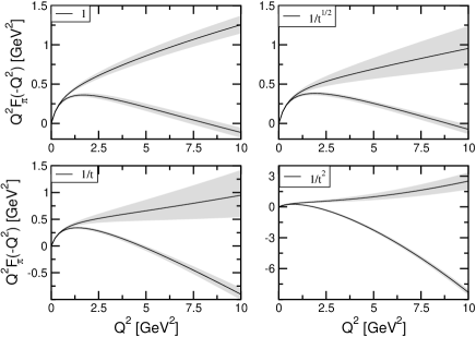
For illustration we show first, in Fig. 1, the upper and lower bounds on the product $Q^{2}\,F(-Q^{2})$ in the range $0\leq Q^{2}\leq 10\,\,\text{GeV}^{2}$, obtained with different weight functions, using as input the relations (3), (4) and (7), with no information from the spacelike axis. The solid lines are the bounds for the central values of the input, and the grey bands indicate the uncertainty on the corresponding bounds, obtained by adding in quadrature the uncertainties due to the variation of the phase given in (22), the charge radius $\langle r_{\pi}^{2}\rangle$ given in (23), and the integral $I$ from Table 1.

The results obtained with different weights are rather similar, except for the weight $\rho_{2}(t)$, which gives much weaker bounds at high $Q^{2}$. This feature is actually expected: since this weight decreases rapidly, the class of functions satisfying (4) is less constrained at high energies, even functions increasing asymptotically being accepted. We note that in the so-called unitarity bounds approach, applied to the pion form factor in [59, 63], an inequality similar to (4) is derived from a dispersion relation for a physical observable, like a polarization function calculated in perturbative QCD or the hadronic contribution to the muon anomaly, using in addition unitarity for the corresponding spectral function. In this approach the effective weight $\rho(t)$ is fixed and cannot be chosen at will, decreasing actually like $1/t^{2}$ in all the cases investigated. Therefore, as discussed in [63], the approach of unitarity bounds, which is useful when no information on the modulus is available, would give weak bounds on the pion form factor at higher energies on the spacelike axis. The recent high statistic measurements of the modulus up to rather high energies on the timelike axis [44] allow us to choose an optimal weight, leading to a remarkable improvement of the bounds on the spacelike axis.

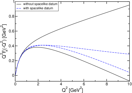
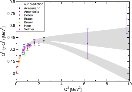
In Fig. 2 we demonstrate the effect of an additional input from the spacelike datum (24), using for illustration the weight $\rho_{1/2}(t)$. The solid lines show the bounds obtained as before without any spacelike information, while the dashed lines are obtained by imposing the central value from (24). The inclusion of this additional information narrows considerably the allowed domain situated between the upper and the lower bounds.

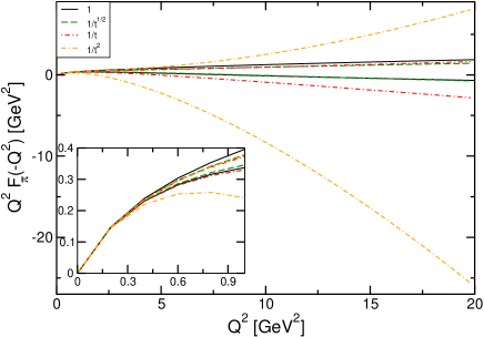
The comparison of various weights is seen in Fig. 3, where the bounds are again obtained with the central input values, including the spacelike datum from (24). At low $Q^{2}$ the bounds obtained with different weights are almost identical, and are very tight. At higher $Q^{2}$ the small constraining effect of the weight $\rho_{2}(t)$ is again visible, while the other weights give comparable results. By inspecting the curves, we conclude that the best results are obtained with the weight $\rho_{1/2}(t)$, and we shall adopt this weight in what follows. In fact, it gives bounds almost identical with the weight $\rho_{1}(t)\equiv 1$. In addition, it has the advantage of being less sensitive to the unknown high-energy behavior of the form factor, as discussed in the previous section in connection with the calculation of the quantities $I$ given in Table 1.

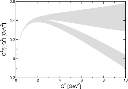
In Fig. 4 we illustrate, for the special weight $\rho_{1/2}(t)$, the effect of the uncertainties of the input on the resulting bounds. Since we are interested in the most conservative results, i.e., the largest allowed domain defined by the upper and the lower bounds, it is enough to exhibit the upward shift of the upper bound, and the downward shift of the lower bound, produced by the uncertainties of the input. By including these uncertainties, the allowed domain obtained with the central input, shown as the inner white region in Fig.4, is enlarged covering the large grey domains. We recall that in each point the error is obtained by adding quadratically the errors produced by the variation of the phase (22), the charge radius (23), the integral $I$ for $a=1/2$ from Table 1, and the experimental value given in (24).

It turns out that the greatest contribution to the size of the grey domain is the experimental uncertainty of the spacelike value (24), which decreases the lower bound by about 30% for values of $Q^{2}$ around $7\,\text{GeV}^{2}$, for instance. This shows that more accurate experimental data or lattice calculations at some points on the spacelike axis will lead to more stringent constraints in this region, which, as shown below, is of interest for the onset of the perturbative QCD regime. At larger values of $Q^{2}$, the effect of the uncertainty in the charge radius starts to increase, becoming of comparable value, of about $30\%$, near $Q^{2}=10\,\text{GeV}^{2}$. The uncertainty of the integral $I$ has an effect of less than 8% in the considered range (as expected, it has a noticeable effect only at higher momenta).

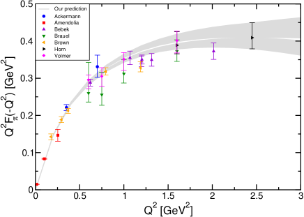
In Figs. 5 and 6, we compare the constraints corresponding to the weight $\rho_{1/2}(t)$ with some of the data available from experiments [38, 39, 36, 32, 34, 30, 31, 29, 35]. We find that at low $Q^{2}$ most of the low-energy data of Amendolia [35] are consistent with the narrow allowed band predicted by our analysis. The most recent data from [38, 39] are well accommodated within our band, which is not surprising as we used one of these points as input. There are however some inconsistencies between the allowed domain derived here and the data of Bebek et al [30, 31], Ackermann et al [32], and Brauel et al [34], in spite of their rather large errors.

Figure 4: Upper and lower bounds derived with the weight $\rho_{1/2}(t)$ by including the charge radius (23) and the spacelike datum (24). Inner white region: allowed domain for the central values of the input. Grey bands: enlarged allowed domain with inclusion of the errors of the input.

Figure 5: Allowed domain obtained with the weight $\rho_{1/2}(t)$ compared with several sets of experimental data.

Figure 6: Enlarged view of Fig. 4 at low energy.

Figure 7: Comparison of the bounds with perturbative QCD and several nonperturbative models.

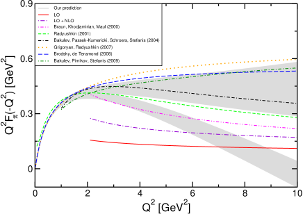
Finally, in Fig. 7 we compare the allowed domain obtained in this work with the predictions of perturbative QCD and several nonperturbative models. We show first the LO expression (1), in which we have taken the scale $\mu^{2}=Q^{2}$ and used the running coupling to one loop

$$\alpha_{s}(Q^{2})=\frac{4\pi}{\beta_{0}\ln(Q^{2}/\Lambda^{2})}.$$ (25)

We have taken $n_{f}=3$ active flavors and $\Lambda=0.214\,\,\text{GeV}$, which in Eq. (25) gives $\alpha_{s}(M_{\tau}^{2})=0.33$, the average of the various predictions from hadronic $\tau$ decays obtained recently [66, 67, 68, 69, 70, 71, 72]. As seen from Fig. 7, the central LO curve, obtained with this choice of the coupling, stays below the lower bound derived in the present work up to $Q^{2}=7\,\,\text{GeV}^{2}$. The variations set by the error of about $\pm 0.02$ in $\alpha_{s}(M_{\tau}^{2})$ quoted in [66, 67, 68, 69, 70, 71, 72] do not modify this conclusion.

As discussed in [12, 10] the perturbative prediction to NLO is sensitive to the choice of the renormalization scale, and also of the factorization scale in the case when pion DAs different from the asymptotic ones are used in the calculation. Several prescriptions for scale setting were adopted, but there is no general consensus on the issue. In particular, in the Brodsky-Lepage-Mackenzie procedure the renormalization scale is chosen such that the coefficient of $\beta_{0}$ in the NLO correction (2) vanishes [12].

For illustration, in Fig. 7 we show the sum of the LO and NLO terms (1) and (2), obtained with the scale $\mu^{2}=Q^{2}$ and the one loop coupling (25). As in previous references [47, 9, 10, 20, 28], we have taken the number of active flavors $n_{f}=3$. This curve is compatible with our bounds enlarged by errors only for $Q^{2}>6\,\,\text{GeV}^{2}$.

When $Q^{2}$ is varied over a large range, one must of course take into account the transition from $n_{f}$ to $n_{f}+1$ active flavors in the $\beta$-function coefficients when the threshold of a new flavor is crossed. However, it turns out that in the region of interest to us, $Q^{2}<10\,\,\text{GeV}^{2}$, the effect of the higher mass quarks is small. First, we recall that the definition of the flavor matching scale is subject to a certain uncertainty. If the thresholds are set at the pole masses of the charm and bottom quarks, $n_{f}$ should be raised to 4 and 5, respectively, when the thresholds of 1.65 GeV and 4.75 GeV are crossed. However, the change in $\beta_{0}$ is small, from $\beta_{0}=9$ to $\beta_{0}=8.33$ for the charm threshold relevant in the region considered. Moreover, the continuity of the coupling (25) must be imposed by a change of the parameter $\Lambda$ above the threshold. Therefore, the modification of the form factor below $Q^{2}=10\,\,\text{GeV}^{2}$ is expected to be quite small and the comparison with the bounds derived in the present paper remains unchanged. We note also that for the choice of the quark-flavor matching scales at $2m_{q}$ as in [66], or at $\mu_{c}^{*}=3.729\,\,\text{GeV}$ and $\mu_{b}^{*}=10.588\,\,\text{GeV}$ as in [67], the thresholds are not crossed and the number of the active flavors remains equal to three in the whole region shown in Fig. 7.

In Fig. 7 we show also several nonperturbative models proposed in the literature for the spacelike form factor at intermediate region [20, 16, 23, 26, 25, 17, 24]

In Ref. [20], the authors applied light-cone QCD sum rules and parametrized with a simple expression the nonperturbative correction, to be added to the LO+NLO perturbative prediction in the region $1<Q^{2}<15\,\,\text{GeV}^{2}$. In Fig. 7 we show the sum of the soft correction and the perturbative QCD prediction to NLO, evaluated at a scale $\mu^{2}=0.5\,Q^{2}+M^{2}$ with $M^{2}=1\,\,\text{GeV}^{2}$ as argued in [20]. The model is quite compatible with our bounds, the corresponding curve being inside the small white inner domain for $Q^{2}>6\,\,\text{GeV}^{2}$.

The model based on local duality [16] is also consistent with the allowed domain derived here for $Q^{2}>1\,\,\text{GeV}^{2}$. We mention that this model, proposed in [14], was recently developed by several authors [17]. The other models shown in Fig. 7 are consistent with the bounds derived by us at low $Q^{2}$, but are at the upper limit of the allowed domain at higher $Q^{2}$. The agreement is somewhat better for the model discussed in [23], which is a LO+NLO perturbative calculation using nonasymptotic pion DAs evolved to NLO, with a modification of the QCD coupling by the so-called analytic perturbation theory. The AdS/QCD model considered in [26] is in fact a simple dipole interpolation, which is valid at low energies but seems to overestimate the form factor at larger momenta. The same remark holds for the models discussed in [24] and [25], based on QCD sum rules with nonlocal condensates, and the chiral limit of the hard-wall AdS/QCD approach, respectively.

VI Discussion and Conclusions

In this paper we derived upper and lower bounds on the pion electromagnetic form factor along the spacelike axis, by exploiting in a conservative way the precise recent information on the phase and modulus on complementary regions of the timelike axis.

More exactly, we have applied a method of analytic continuation which uses as input the phase only in the elastic region $t<t_{\rm in}$, where it is known with high accuracy from the dispersive theory of $\pi\pi$ scattering via the Fermi-Watson theorem. It can be shown rigorously [60] that the results are independent of the unknown phase of the form factor above the first inelastic threshold $t_{\rm in}$. As for the modulus, we have used the BaBar data in the range between the first inelastic threshold and 3 GeV [44], and very conservative assumptions above 3 GeV. The results are not very sensitive to these assumptions, since we include the information on the modulus through the $L^{2}$ integral condition (4), instead of imposing this knowledge pointwise, at each $t$. Obviously, the detailed behavior of $|F(t)|$ is averaged in the integral, and the high-energy contribution can be suppressed by a suitable choice of the weight $\rho(t)$. In our calculations we have choosen a suitable weight, which on the one hand gives sufficiently tight bounds, and on the other hand ensures a small sensitivity to the high energy part. We have found that these constraints are met by a weight of the simple form (6), with the choice $a=1/2$.

We mention that, for completeness, we have investigated also the more general class of weight functions of the form (5) and found, for instance, that with the choices $b=1/2$, $c=1$ and $Q_{0}^{2}$ in the range $3-6\,\,\text{GeV}^{2}$ the bounds are slightly better and have smaller uncertainties than those shown in Fig. 4. For the conclusions formulated in this paper the improvement is not essential. However, a more systematic optimization with respect to the weight is of interest for further studies, especially when more accurate input from the spacelike axis will be available.

Besides the use of the modulus above $t_{\rm in}$ only in an averaged way, as in the condition (4), we note that our method does not exploit completely the present knowledge of the modulus, since we do not use the data on $|F(t)|$ below $t_{\rm in}$. While it may seem that this additional information can improve in a significant way the bounds, it turns out that it is not so. Indeed, the knowledge of the phase below $t_{\rm in}$ has, in the case of the pion form factor, a considerable constraining power on the modulus in the same region. The reason is the strong peak produced by the $\rho$ resonance. The Omnès function ${\cal{O}}(t)$ defined in (9) reproduces well this impressive behavior of the modulus, and this holds for a large class of choices of the arbitrary phase above the elastic region. The effect of this unknown phase is actually completely removed in our formalism by the information on the modulus, which constrains the auxiliary function $h(t)$ appearing in the expression (10) of $F(t)$. Therefore, imposing additional data on $|F(t)|$ below 0.9 GeV is not expected to improve considerably the bounds, if the input values of the phase and modulus in this region are consistent. Of course, one can reverse the argument and find constraints on the modulus on the timelike axis below $t_{\rm in}$, in order to test the consistency. This analysis will be carried out in the future.

In the present work we have investigated the consistency of the timelike phase and modulus with the experimental data and theoretical models on the spacelike axis. The slow onset of the asymptotic regime predicted by factorization and perturbative QCD for the pion electromagnetic form factor has been known for a long time. A lot of theoretical work has been done by several groups on the determination of the pion form factor in the spacelike intermediate energy region, where the soft, nonperturbative contributions are expected to be important. However, definite conclusions on the validity of the theoretical models and the precise energy at which the asymptotic regime may be considered valid were not possible, due to the lack of accurate experimental data in the relevant region.

The bounds derived in the present paper are almost model-independent and very robust, allowing us to make some definite statements. From Fig. 7 it is possible to say with great confidence that perturbative QCD to LO is excluded for $Q^{2}<7\,\,\text{GeV}^{2}$, and perturbative QCD to NLO is excluded for $Q^{2}<6\,\,\text{GeV}^{2}$, respectively. If we restrict to the inner white allowed domain obtained with the central values of the input, the exclusion regions become $Q^{2}<9\,\,\text{GeV}^{2}$ and $Q^{2}<8\,\,\text{GeV}^{2}$, respectively. Among the theoretical models, the light-cone QCD sum rules [20] and the local quark-hadron duality model [16] are consistent with the allowed domain derived here for a large energy interval, while the remaining models are consistent with the bounds at low energies, but seem to predict too high values at higher $Q^{2}$.

To increase the strength of the predictions, a reduction of the grey bands produced by the uncertainties of the input is desirable. As we mentioned, the biggest contribution is brought by the experimental errors of the input spacelike datum (24). Therefore, more accurate data at a few spacelike points, particularly at larger values of $Q^{2}$ will be very important for increasing the predictive power of the formalism developed and applied in the present paper.

Acknowledgement: IC acknowledges support from CNCS in the Program Idei, Contract No. 121/2011. We thank B. Malaescu for correspondence on the BaBar data and S.Dubni$\check{c}$ka for discussions.

References

- [1] G.R. Farrar and D.R. Jackson, Phys. Rev. Lett. 43, 246 (1979).
- [2] G.P. Lepage and S.J. Brodsky, Phys. Lett. B 87, 359 (1979).
- [3] A.V. Efremov and A.V. Radyushkin, Phys. Lett. B 94, 245 (1980).
- [4] V.L. Chernyak, A.R. Zhitnitsky and V.G. Serbo JETP Lett. 26 594 (1977) [Pisma Zh. Eksp. Teor.Fiz. 26 760-763 (1977)].
- [5] R. D. Field, R. Gupta, S. Otto and L. Chang, Nucl. Phys. B 186, 429 (1981).
- [6] F. M. Dittes and A. V. Radyushkin, Sov. J. Nucl. Phys. 34, 293 (1981) [Yad. Fiz. 34, 529 (1981)].
- [7] R. S. Khalmuradov and A. V. Radyushkin, Sov. J. Nucl. Phys. 42, 289 (1985) [Yad. Fiz. 42, 458 (1985)].
- [8] E. Braaten and S. M. Tse, Phys. Rev. D 35, 2255 (1987).
- [9] B. Melic, B. Nizic and K. Passek, Phys. Rev. D 60, 074004 (1999) [arXiv:hep-ph/9802204].
- [10] B. Melic, B. Nizic and K. Passek, arXiv:hep-ph/9908510.
- [11] Hsiang-nan Li, Yue-Long Shen, Yu-Ming Wang, and Hao Zou, Phys. Rev. D 83, 054029 (2011) [arXiv:1012.4098 [hep-ph]]
- [12] S.J. Brodsky, C.-R. Ji, A. Pang and D.G. Robertson, Phys. Rev. D 57, 245 (1998) [hep-ph/9705221].
- [13] B.L. Ioffe and A.V. Smilga, Phys. Lett. B 114, 353 (1982).
- [14] V. A. Nesterenko and A. V. Radyushkin, Phys. Lett. B 115, 410 (1982).
- [15] A.V. Radyushkin, Acta Phys. Polon. B 26, 2067 (1995) [hep-ph/9511272].
- [16] A.V. Radyushkin, Proceedings of the Chiral dynamics 2000, Newport News, Virginia, pag. 309-311, hep-ph/0106058.
- [17] V. Braguta, W. Lucha and D. Melikhov, Phys. Lett. B 661, 354 (2008) [arXiv:0710.5461 [hep-ph]].
- [18] C.A. Dominguez, Phys. Rev. D 25, 3084 (1982).
- [19] V.M. Braun and I.E. Halperin, Phys. Lett. B 328, 457 (1994) [hep-ph/9402270].
- [20] V.M. Braun, A. Khodjamirian and M. Maul, Phys. Rev. D 61, 073004 (2000) [arXiv:hep-ph/9907495].
- [21] J. Bijnens and A. Khodjamirian, Eur. Phys. J. C 26, 67 (2002) [arXiv:hep-ph/0206252].
- [22] A.P. Bakulev and A.V. Radyushkin, Phys. Lett. B 271, 223 (1991).
- [23] A.P. Bakulev, K. Passek-Kumericki, W. Schroers and N.G. Stefanis, Phys. Rev. D 70, 033014 (2004) [Erratum-ibid. D 70, 079906 (2004)] [arXiv:hep-ph/0405062].
- [24] A.P. Bakulev, A.V. Pimikov and N.G. Stefanis, Phys. Rev. D 79, 093010 (2009) [arXiv:0904.2304 [hep-ph]].
- [25] H.R. Grigoryan and A.V. Radyushkin, Phys.Rev.D 76, 115007 (2007) [arXiv:0709.0500 [hep-ph]].
- [26] S.J. Brodsky and G.F. de Teramond, Phys. Rev. D 77, 056007 (2008) [arXiv:0707.3859 [hep-ph]].
- [27] T. Gousset and B. Pire, Phys. Rev. D 51, 15 (1995) [hep-ph/9403293].
- [28] E. Ruiz Arriola and W. Broniowski, Phys. Rev. D 78, 034031 (2008) [arXiv:0807.3488 [hep-ph]].
- [29] C.N. Brown, C.R. Canizares, W.E. Cooper, A.M. Eisner, G.J. Feldmann, C.A. Lichtenstein, L. Litt, W. Loceretz, V.B. Montana and F.M. Pipkin Phys. Rev. D 8, 92 (1973).
- [30] C.J. Bebek, C.N. Brown, M. Herzlinger, Stephen D. Holmes, C.A. Lichtenstein, F.M. Pipkin, L.K. Sisterson, D. Andrews, K. Berkelman and D.G. Cassel, Phys. Rev. D 9, 1229 (1974).
- [31] C.J. Bebek, C.N. Brown, M. Herzlinger, Stephen D. Holmes, C.A. Lichtenstein, F.M. Pipkin, S. Raither and L.K. Sisterson, Phys. Rev. D 13, 25 (1976).
- [32] H. Ackermann, T. Azemoon, W. Gabriel, H.D. Mertiens, H.D. Reich, G. Specht, F. Janata and D. Schmidt, Electroproduction,” Nucl. Phys. B 137, 294 (1978).
- [33] C.J. Bebek et al.,’ Phys. Rev. D17, 1693 (1978).
- [34] P. Brauel, T. Canzler, D. Cords, R. Felst, G. Grindhammer, M. Helm, W.D. Kollmann and H. Krehbiel, Z. Phys. C 3, 101 (1979).
- [35] S.R. Amendolia et al. [NA7 Collaboration], Nucl. Phys. B 277, 168 (1986).
- [36] J. Volmer et al. [The Jefferson Lab F(pi) Collaboration], Phys. Rev. Lett. 86, 1713 (2001) [arXiv:nucl-ex/0010009].
- [37] V. Tadevosyan et al. [Jefferson Lab F(pi) Collaboration], Phys. Rev. C 75, 055205 (2007) [arXiv:nucl-ex/0607007].
- [38] T. Horn et al. [Jefferson Lab F(pi)-2 Collaboration], Phys. Rev. Lett. 97, 192001 (2006) [arXiv:nucl-ex/0607005].
- [39] G.M. Huber et al. [Jefferson Lab Collaboration], Phys. Rev. C 78, 045203 (2008) [arXiv:0809.3052 [nucl-ex]].
- [40] B. Ananthanarayan, G. , J. Gasser and H. Leutwyler, Phys. Rept. 353, 207 (2001) [arXiv:hep-ph/0005297].
- [41] G. Colangelo, J. Gasser and H. Leutwyler, Nucl. Phys. B 603, 125 (2001) [arXiv:hep-ph/0103088].
- [42] R. Garcia-Martin, R. Kaminski, J.R. Pelaez, J.Ruiz de Elvira and F.J. Yndurain, Phys. Rev. D 83, 074004 (2011) [arXiv:1102.2183 [hep-ph]].
- [43] I Caprini, G. Colangelo and H. Leutwyler, Eur. Phys. J.C 72, 1860 (2012) [arXiv:1111.7160 [hep-ph]].
- [44] B. Aubert et al. [BABAR Collaboration], Phys. Rev. Lett. 103, 231801 (2009) [arXiv:0908.3589 [hep-ex]].
- [45] F. Ambrosino et al. [KLOE Collaboration], Phys. Lett. B 670, 285 (2009) [arXiv:0809.3950 [hep-ex]].
- [46] F. Ambrosino et al. [KLOE Collaboration], Phys.Lett. B 700, 102 (2011) [arXiv:1006.5313 [hep-ex]].
- [47] J.F. Donoghue and E.S. Na, Phys. Rev. D 56, 7073 (1997) [arXiv:hep-ph/9611418].
- [48] M. Belicka, S. Dubnicka, A.Z. Dubnickova and A. Liptaj, Phys. Rev. C 83, 028201 (2011) [arXiv:1102.3122 [hep-ph]].
- [49] J.F. De Trocóniz and F.J. Yndurain, Phys. Rev. D 65, 093001 (2002) [arXiv:hep-ph/0106025].
- [50] F. Guerrero and A. Pich, Phys. Lett. B 412, 382 (1997) [arXiv:hep-ph/9707347].
- [51] A. Pich and J. Portoles, Phys. Rev. D 63, 093005 (2001) [arXiv:hep-ph/0101194].
- [52] B.V. Geshkenbein, Phys. Rev. D 61, 033009 (2000) [arXiv:hep-ph/9806418].
- [53] W.W. Buck and R.F. Lebed, Phys. Rev. D 58, 056001 (1998) [arXiv:hep-ph/9802369].
- [54] C.B. Lang and I.S. Stefanescu, Phys. Lett. B 58, 450 (1975).
- [55] M.F. Heyn and C.B. Lang, Z. Phys. C 7, 169 (1981).
- [56] G. Colangelo, Nucl. Phys. Proc. Suppl. 131, 185 (2004) [arXiv:hep-ph/0312017].
- [57] P. Masjuan, S. Peris and J.J. Sanz-Cillero, Phys. Rev. D 78, 074028 (2008) [arXiv:0807.4893 [hep-ph]].
- [58] H. Leutwyler, arXiv:hep-ph/0212324.
- [59] I. Caprini, Eur. Phys. J. C 13, 471 (2000) [arXiv:hep-ph/9907227].
- [60] G. Abbas, B. Ananthanarayan, I. Caprini, I.Sentitemsu Imsong and S. Ramanan, Eur. Phys. J. A 45, 389 (2010), [arXiv:1004.4257 [hep-ph]].
- [61] G. Abbas, B. Ananthanarayan, I. Caprini, I. Sentitemsu Imsong and S. Ramanan, Eur. Phys. J. A 44, 175 (2010) [arXiv:0912.2831 [hep-ph]].
- [62] G. Abbas, B. Ananthanarayan, I. Caprini and I. Sentitemsu Imsong, Phys. Rev. D 82, 094018 (2010) [arXiv:1008.0925 [hep-ph]].
- [63] B. Ananthanarayan, I. Caprini and I.S. Imsong, Phys. Rev. D 83, 096002 (2011) [arXiv:1102.3299 [hep-ph]].
- [64] B. Ananthanarayan, I. Caprini and I. Sentitemsu Imsong, Eur. Phys. J. A 47, 147 (2011) [arXiv:1108.0284 [hep-ph]].
- [65] H. Cornille and A. Martin, Nucl. Phys. B 93, 61 (1975).
- [66] M. Davier, S. Descotes-Genon, A. Höcker, B. Malaescu, and Z. Zhang, Eur. Phys. J. C56, 305 (2008) [arXiv:0803.0979 [hep-ph]].
- [67] M. Beneke and M. Jamin, JHEP 0809, 044 (2008) [arXiv:0806.3156 [hep-ph]].
- [68] I. Caprini and J. Fischer, Eur. Phys. J. C 64, 35 (2009) [arXiv:0906.5211 [hep-ph]].
- [69] I. Caprini and J. Fischer, Phys. Rev. D84:054019 (2011) [arXiv:1106.5336 [hep-ph]].
- [70] S. Bethke et al, Workshop on Precision Measurements of , arXiv:1110.0016.
- [71] D. Boito, O. Cata, M. Golterman, M. Jamin, K. Maltman, J. Osborne and S. Peris, Phys. Rev. D84, 113006 (2011) [arXiv:1110.1127 [hep-ph]].
- [72] G. Abbas, B. Ananthanarayan and I. Caprini, arXiv:1202.2672 [hep-ph].