Non-linear power spectra of dark and luminous
matter in halo model of structure formation

Abstract

The late stages of large-scale structure evolution are treated semi-analytically within the framework of modified halo model. We suggest simple yet accurate approximation for relating the non-linear amplitude to linear one for spherical density perturbation. For halo concentration parameter, $c$, a new computation technique is proposed, which eliminates the need of interim evaluation of the $z_{col}$. Validity of the technique is proved for $\Lambda$CDM and $\Lambda$WDM cosmologies. Also, the parameters for Sheth-Tormen mass function are estimated. The modified and extended halo model is applied for determination of non-linear power spectrum of dark matter, as well as for galaxy power spectrum estimation. The semi-analytical techniques for dark matter power spectrum are verified by comparison with data from numerical simulations. Also, the predictions for the galaxy power spectra are confronted with ’observed’ data from PSCz and SDSS galaxy catalogs, good accordance is found.

I Introduction

A commonly accepted inflationary paradigm states that the large-scale structure (LSS) of the Universe is formed through evolution of density perturbations driven by gravitational instability. At some moment the growth of small-scale perturbations switches to non-linear regime. The treatment of linear regime is quite simple, the linear power spectrum (transfer function) for $k<0.1$ h/Mpc can be readily computed with percent accuracy for any feasible cosmology. However, it is not so for the smaller scales, due to the non-linear terms in equations and complexity of physics of baryonic component (hydrodynamics, radiation transfer, thermal and chemical evolution). This paper is aimed for the development of technique capable to build a bridge between the initial (linear) matter power spectrum and observable (inherently non-linear) galaxy power spectrum. The treatment is based on halo model complemented by analytical approximations, the results are tested and verified against data of N-body simulations.

Within the scenario commonly referred as “standard” (see b71 ), the gravitational potential of collisionless dark matter inhomogeneities governs the baryonic matter until the baryonic matter power spectrum reaches the dark matter’s one in amplitude. At some moment, a non-linear perturbation with amplitude exceeding some critical one detaches from background expansion, reaches a turnaround point and starts to collapse due to self-gravity. Subsequently the violent relaxation takes place, which brings the system into the virial equilibrium, so the halo of dark matter is formed. Then, the baryonic gas starts to cool down, followed by clumping into clouds and ignition of the luminous tracers within halos (see b4 ; b6 for details).

Thus, the spatial distribution of luminous matter should strongly correlate with one of halos. The correlation is confirmed by large simulations, which take into account the baryon physics and particle dynamics of dark matter b57 ; b58 , and by semi-analytic models of galaxy formation b59 ; b60 ; b61 as well. The numerical techniques require the considerable computing power, whereas the purely analytical are found unreliable and inaccurate. Thus, the “hybrid” approach seems to be optimal, combining the analytical model of galaxy formation b62 ; b63 with dark matter “merger trees” extracted from simulations. Another way is to extract the halo and subhalo statistics from simulations for comparison with galaxy populations in large galaxy survey. Such techniques are based on conditional luminosity function (CLF) b19 ; b32 ; b33 , conditional mass function (CMF) b20 and stellar mass to halo mass relation b1 ; b20 .

The halo model is a cornerstone of modern theory of structure formation. It has been proven to be well-motivated, comprehensive and provides plausible explanation for observational data and results of cosmological simulations. It is valid for wide range of cosmologies, as long as the statistics of primordial density perturbations is Gaussian. It encompasses the non-linear stage of evolution of density perturbations as well as the dynamical relaxation processes assuming that the whole mass is associated with gravitationally bound virialized halo.

It has shown in papers b7 ; b70 ; b65 that the dark matter non-linear power spectrum can be evaluated given halo statistics, their internal structure and spatial distribution. Also vice versa, the initial power spectrum can be reconstructed by applying the halo model to the data of N-body simulations. As another example, the halo occupation function, $p(N|M)$, probability of finding $N$ galaxies within a halo of mass $M$, was used in b67 ; r03 along with halo model to calculate the non-linear galaxy power spectrum. However, regardless of overall success of the halo model in description of dark matter and galaxy clustering, it is still not to be considered as complete. For instance, only the latest enhancements proposed in b29 ; r04 take into account the internal structure of halo as well as the halo shapes r05 ; r06 .

To apply the halo model, the a priori knowledge of the evolution of inhomogeneities from initial state through collapse to the formation of virialized halo is required. In section II we analyze such evolution using the spherical perturbation model in order to analytically relate the amplitude of non-linear spherical density perturbation to the one of the linear. Also, the new technique is proposed therein for computation of concentration parameter $c$ for halo with Navarro-Frenk-White density profile. In section III the halo mass function is applied to the dark matter clustering. In section IV the galaxy power spectra are estimated and compared to ’observable’ ones, as derived in b26 ; b27 from PSCz and SDSS catalogs. The conclusions are presented in section V. The computations were performed for $\Lambda$CDM (cold dark matter with $\Lambda$-term) and $\Lambda$WDM (warm dark matter with $\Lambda$-term) cosmological models, some bulk mathematical derivations are separated in appendices.

II Formation of individual spherical halo

II.1 Spherical overdensity with arbitrary profile

In the framework of Tolman’s approach b78 , the spherically symmetrical inhomogeneity is treated in synchronous gauge (i.e. with regard to the frame comoving to the dust-like matter component), with space-time interval

$$ds^{2} = dt^{2}-\frac{y^{2}(t,R)}{\sqrt{1-KR^{2}}}dR^{2}$$ (1)

$$-x^{2}(t,R)R^{2}\left(d\theta^{2}+\sin^{2}\theta d\varphi^{2}\right),$$

where $t$ is a proper time of an observer located at $R$, $K$ is space curvature of the Universe as the whole. For homogeneous Friedmann Universe $x(t)=y(t)=a(t)$.

The mean matter density, i.e. average value over the sphere of radius $R$, is denoted by $\rho_{M}(\tau,R)\equiv\rho_{m}^{0}x^{-3}(\tau,R)$, and the matter density at some specific distance $R$ from the center of perturbation is $\rho(\tau,R)\equiv\rho_{m}^{0}x^{-2}(\tau,R)y^{-1}(\tau,R)$, see b17 ; b17a for details. Let us define the amplitude of density perturbation as follows:

$$\delta_{\rho}(t,R)=\frac{\rho(t,R)-\overline{\rho}(t)}{\overline{\rho}(t)}=\frac{a^{3}(t)}{x^{2}(t,R)y(t,R)}-1,$$ (2)

the amplitude of the mass perturbation is

$$\delta_{M}(t,R)=\frac{\rho_{M}(t,R)-\overline{\rho}(t)}{\overline{\rho}(t)}=\frac{a^{3}(t)}{x^{3}(t,R)}-1.$$ (3)

These amplitudes (see b17 ) are related by

$$\delta_{M}(t,R)=\frac{3}{r^{3}(t,R)}\int_{0}^{R}\delta_{\rho}(t,R)r^{2}(t,R)r^{\prime}(t,R)dR$$ (4)

with $r(t,R)=x(t,R)R$, $(^{\prime})\equiv d/dR$.

For small perturbations the following approximations are valid for (2) and (3):

$$\delta_{\rho}(t,R) \simeq \delta(t,R)\equiv A(R)D\left(a(t)\right)\ll 1,$$ (5)

$$\delta_{M}(t,R) \simeq \overline{\delta}(t,R)\equiv\frac{3}{5}\frac{\Omega_{K}-\Omega_{f}(R)}{\Omega_{m}}\,D\left(a(t)\right)\ll 1,$$ (6)

were $D(a(\tau))$ is the growth factor of linear matter density perturbations b12 ; b18 , defined by

$$D(a)=\frac{5}{2}\Omega_{m}a^{-1}X^{1/2}(a)\int_{0}^{a}X^{-3/2}(\tilde{a})d\tilde{a},$$ (7)

where $X(a)\equiv\Omega_{\Lambda}a^{2}+\Omega_{m}a^{-1}+\Omega_{K}$. The parameter of local curvature, $\Omega_{f}(R)$, can be related due to Eq. (4) with the density profile, $A(R)$, from (6) as

$$\Omega_{f}(R)=-5\Omega_{m}R^{-3}\int\limits_{0}^{R}A(\tilde{R})\tilde{R}^{2}d\tilde{R}+\Omega_{K}.$$ (8)

Thus, either $A(R)$ or $\Omega_{f}(R)$ should be specified to define the initial profile of perturbation.

The Einstein’s equations for spherical overdensity of dust-like matter in the model with cosmological constant, $\mathcal{G}^{1}_{1}=\mathcal{G}^{2}_{2}=\Lambda$, yield the equations for $x(\tau,R)$ and $y(\tau,R)$:

$$\ddot{x} = \frac{3}{2}\Omega_{\Lambda}x-\frac{1}{2}\frac{\dot{x}^{2}}{x}+\frac{1}{x}\frac{\Omega_{f}}{2},$$ (9)

$$\ddot{y} = \frac{3}{2}\Omega_{\Lambda}y-\left(\frac{\dot{x}\dot{y}}{x}-\frac{1}{2}\frac{\dot{x}^{2}y}{x^{2}}\right)+\left(\Omega_{f}+R\frac{\Omega_{f}^{\prime}}{2}\right)\frac{1}{x}-\frac{y}{x^{2}}\frac{\Omega_{f}}{2}$$

The overdot denotes a derivative with respect to $\tau=H_{0}t$. The first integration of (9) yields

$$\dot{x}^{2}-\frac{\Omega_{m}}{x}-\Omega_{\Lambda}x^{2}=\Omega_{f}.$$ (11)

Thus, the amplitude of mass perturbation, (3), can be calculated by integrating over the time just this single equation.

The development of spherical inhomogeneity can be divided into two stages: 1) the expansion stage ($\dot{x}>0$, $\dot{\rho}_{M}<0$), linear and weakly non-linear regime; 2) the collapse stage ($\dot{x}<0$, $\dot{\rho}_{M}>0$), entirely non-linear regime. They are separated by the moment of turnaround, when $\dot{x}=0$ ($\dot{\rho}_{M}=0$).

The evolution of perturbation at non-linear stage is convenient to be treated by confronting with the evolution of some fictitious linear perturbation extrapolated beyond the linear stage. Therefore, the time dependence is represented in terms of the ratio of $\overline{\delta}$, the initial mean overdensity of linear perturbation at some $R$, to the $\delta_{col}$, critical overdensity b16 ; b18 ; b17 , the amplitude of perturbation which is to collapse at the moment $t_{col}$.

Figure 1: Top panel: the dependence of non-linear amplitude of spherical perturbation on the linear one. Bottom panel: the accuracy of the approximation (12) for some cosmological models, where $\delta^{appr}_{M}$ denotes the right hand side of (12) and $\delta_{M}$ is the exact value.

In the Fig. 1 the dependence of non-linear amplitude on the ratio $\overline{\delta}/\delta_{col}$ is plotted, as computed by integration of Eqs. (11) and (LABEL:Per2). The fit for the dependence is simple,

$$\lg\left[1+\delta_{M}\right] \simeq -\delta_{col}\cdot\lg\left[1-\overline{\delta}/\delta_{col}\right]+A\cdot\lg^{2}\left[1-\overline{\delta}/\delta_{col}\right]$$ (12)

$$+ B\cdot\lg^{3}\left[1-\overline{\delta}/\delta_{col}\right],$$

the coefficients are $A=0.0903$ and $B=0.0074$. This fit is similar to the proposed by r01 , wherein the values $A=0$ and $B=0$ were assumed, see also r02 . The fitting errors do not exceed 1% until the moment of complete collapse, when $\delta_{M}\rightarrow\infty$ (bottom panel of Fig. 1).

Given $\delta_{M}$, the density amplitude, $\delta_{\rho}$, is to be evaluated at any radius $R$ with

$$\delta_{\rho}=\frac{1+\delta_{M}}{1+(\overline{\delta}-\delta)\frac{\partial}{\partial\overline{\delta}}\ln(1+\delta_{M})}-1.$$ (13)

II.2 Virialization and final parameters of individual spherical halo

Figure 2: The dependence of virialized spherical cloud density on $\Omega_{m}$ in units of the critical density at the moment of collapse, $\Delta_{vc}$, for models with fixed $\Omega_{\Lambda}$, (a), and $\Omega_{K}$, (b).

Note that the true singularity at collapse stage in the center of the overdensity as a rule is not reached, since the falling of particles usually is not strictly radial and small-scale inhomogeneities within the cloud induce the additional non-radial velocities of particles. The process of virialization is far from trivial, however, when the relaxation is finished and dynamical equilibrium is established, the kinetic energy and the gravitational potential satisfy the virial theorem. For instance, for a spherical relaxed halo the kinetic energy per unit mass is determined by

$$T_{vir}/m=\frac{1}{2}\left<v^{2}\right>_{vir}=\frac{1}{2}r\frac{\partial U_{vir}}{\partial r}.$$

For $\Lambda$CDM model $U_{vir}=-H_{0}^{2}\Omega_{\Lambda}x_{vir}^{2}-H_{0}^{2}\Omega_{m}/x_{vir}$ b18 and the total energy of isolated dark matter cloud is conserved. By equating the total energy at turnaround point (kinetic energy is zero and $E_{tot}=U_{ta}$) to the one at virialization epoch ($E_{tot}=U_{vir}+T_{vir}$) we obtain

$$2\Omega_{\Lambda}x_{vir}^{2}+\frac{1}{2}\frac{\Omega_{m}}{x_{vir}}=\Omega_{\Lambda}x_{ta}^{2}+\frac{\Omega_{m}}{x_{ta}}.$$ (14)

With Eq. (11) for turnaround point, $\dot{x}(\tau_{ta})=0$, we get the cubic equation for $x_{vir}$,

$$4\Omega_{\Lambda}x_{vir}^{3}+2\Omega_{f}x_{vir}+\Omega_{m}=0,$$ (15)

with real root for overdensity ($\Omega_{f}<0$) in cosmology with $\Omega_{\Lambda}>0$,

$$x_{vir}=\left(-\frac{2\Omega_{f}}{3\Omega_{\Lambda}}\right)^{\frac{1}{2}}\cos\left\{\frac{1}{3}\arccos\left[-\frac{\Omega_{m}}{8\Omega_{\Lambda}}\left(-\frac{6\Omega_{\Lambda}}{\Omega_{f}}\right)^{\frac{3}{2}}\right]-\frac{2\pi}{3}\right\}.$$ (16)

For $\Omega_{\Lambda}=0$, the Eq. (14) implies the strict equality $x_{vir}=x_{ta}/2$. For $\Omega_{\Lambda}>0$, $x_{vir}<x_{ta}/2$, albeit the difference is not large. In fiducial model with $\Omega_{\Lambda}=0.7$ and $\Omega_{m}=0.3$ for perturbation collapsing at current epoch, the relative difference $(\frac{1}{2}x_{ta}-x_{vir})/x_{vir}$ is indeed $\sim 0.1$ and diminishes with either $\Omega_{\Lambda}$ decrease or increase of collapse redshift. Therefore, the approximation $x_{vir}\approx x_{ta}/2$ can be applied in most cases.

Note, that the value of $x_{vir}$ depends on the local curvature $\Omega_{f}$ and consequently on the collapse time, $t_{col}$. Also, the virial mass density, $\rho_{vir}=\rho_{m}^{0}x_{vir}^{-3}$, depends on $t_{col}$. It is convenient to represent the virial density in units of critical one, taken at the moment of collapse:

$$\Delta_{vc}=\frac{\rho_{vir}(\tau_{col})}{\rho_{cr}(\tau_{col})}=\frac{\Omega_{m}H_{0}^{2}}{x_{vir}^{3}(\tau_{col})H^{2}(\tau_{col})}.$$ (17)

For the Einstein–de Sitter model ($\Omega_{m}=1$, $\Omega_{\Lambda}=0$) this ratio does not depend on the collapse moment and equals $\Delta_{vc}=18\pi^{2}\simeq 178$.

III Density profiles and concentration parameter

The basic assumption of halo model is that dark matter is associated with virialized halos, which have some universal density profile. Halo density profile is described by generic expression, $\rho(r)=\rho_{s}(r/r_{s})^{-\gamma}(1+r/r_{s})^{\gamma-\alpha}$, with coefficients restricted by b73 to $2.5\leq\alpha\leq 3$ and $1\leq\gamma\leq 1.5$. The characteristic radius $r_{s}$ specifies the distance, at which the slope of density profile changes. We use universal NFW density profile b16 henceforth, this is a special case of generic profile with values of slopes fixed as $\gamma=1$ and $\alpha=3$:

$$\rho(r)=\frac{\rho_{s}}{(r/r_{s})(1+r/r_{s})^{2}}.$$ (18)

For this density profile the total halo mass diverges logarithmically with $r$, whence the size of each halo has to be limited to some finite value.

The characterization of halo is a matter of convention. Here, the mass of halo is defined as a mass of the whole matter contained within the volume of radius $r_{vir}$. The quantity $r_{vir}$ is defined as a radius of sphere, the mean internal density of which exceeds the value of the critical density by some fixed factor. In case of the factor $200$ the halo mass is denoted by $M_{200}$, for $\Delta_{vc}$ used as a factor the $M_{\Delta}$ is a denotation of halo mass. Sometimes the factor is assumed to be $180$, so that the $M_{180}$ is used accordingly. The index is omitted when the choice of definition is clear from context.

The ratio of radius $r_{vir}$, used at defining the halo, to the quantity $r_{s}$ is called the concentration parameter (or just concentration) and denoted as $c$. Depending on the definition of $r_{vir}$, the corresponding index is used as $c_{200}$, $c_{\Delta}$, $c_{180}$. By defining the mass of halo and concentration parameter, one defines the parameters of halo profile, $\rho_{s}$ and $r_{s}$.

For halos of fixed mass the concentration is a stochastic variable, with log-normal probability distribution function,

$$p(c|m,z)dc=\frac{1}{\sqrt{2\pi}\sigma_{\ln c}}\exp\left[-\frac{\ln^{2}[c/\overline{c}(m,z)]}{2\sigma_{\ln c}^{2}}\right]d\ln c.$$ (19)

In such case the variance of concentration virtually does not depend on the halo mass ($\sigma_{\ln c}=0.2-0.35$, see b84 ), whereas the mean value of concentration depends on mass and redshift. This dependence (the term “mass dependence of concentration” is used hereafter) can be determined either by data of simulations or derived analytically, see b16 ; b86 ; b5 . Since the mass dependence follows from initial power spectrum of matter, the analytical methods seem to be preferable. The changes in mass dependence caused by modifications of shape or normalization of initial power spectrum can be easily taken into account.

Analytical techniques aimed to study the mass dependences of profile parameters are usually based on the treatment of b16 . The data of simulations provide some indications of the growth of profile specific density, $\rho_{s}$, with decrease of halo mass. As it was suggested in b16 , this is due to the tendency of less massive but higher inhomogeneities to collapse earlier. It was assumed also that specific density of halo, $\rho_{s}$, is proportional to the matter density of the Universe, taken for the moment of collapse, i.e.

$$\rho_{s}=C\Omega_{m}\rho_{cr}(1+z_{col})^{3},$$ (20)

with the proportionality constant $C$ to be determined from simulation.

The collapse time is defined in ad-hoc manner. The collapse is assumed to start at some moment of time, “at which half the mass of the halo was first contained in progenitors more massive than some fraction $f$ of the final mass” b83 .

With Press-Schechter formalism this condition implies

$$\mathrm{erfc}\,\left\{\frac{\delta_{col}(z_{col}|z)-\delta_{col}(z|z)}{\sqrt{2(\sigma^{2}(fM|z)-\sigma^{2}(M|z))}}\right\}=\frac{1}{2},$$ (21)

leading to the equation:

$$\delta_{col}(z_{col}|z) = \delta_{col}(z|z)+C^{\prime}\sqrt{\sigma^{2}(fM|z)-\sigma^{2}(M|z)}$$ (22)

$$\simeq \delta_{col}(z|z)+C^{\prime}\sigma(fM|z),$$

where $\sigma^{2}(M|z)=\sigma^{2}(M)(D(z)/D(0))^{2}$ and $\sigma^{2}(M)\equiv\sigma^{2}(M|z=0)$. Here, $z$ is the moment of halo observation, $C^{\prime}\approx 0.7$, the term $\sigma^{2}(M|z)$ was neglected in comparison with $\sigma^{2}(fM|z)$. The values of $C$ and $f$ ought to be driven from simulation data. In b16 , $f$ was found to be virtually independent of cosmological parameters at $\approx 0.01$, meanwhile the coefficient $C\sim 10^{3}$, and is strongly determined by the background cosmological model and/or initial power spectrum.

As far as $C$ and $f$ have been determined, the specific density of halo, $\rho_{s}$, can be estimated by Eqs. (22) and (20) for given halo mass $M$ as well as other halo parameter, $r_{s}$. Since there is no explicit analytical expression for dependence $\delta_{col}(z_{col}|z)$ in such treatment, it ought to be recomputed for each cosmology. Therefore, the following simplification of Eq. (22) had been proposed in b86 :

$$\sigma(fM_{\Delta}|z_{col})=1.686,\,\mbox{with}\,\,f=0.01.$$ (23)

Also, the simple approximation was proposed therein for the concentration, $c_{\Delta}=K(1+z_{col})/(1+z)$, with $K$ estimated from numerical modeling as $K=4$.

As it was shown in b5 , the above mentioned estimation of concentration parameter from power spectra is applicable to CDM cosmology. However, it is not a case for Warm Dark Matter (WDM), since wrong dependences follow from it for smaller scales. According to the computer simulations b5 ; r08 , for WDM the concentration tends to grow with the mass increase, whereas for the CDM the contrary dependence is expected.

Since the power spectrum and mass dependence of concentration share the same behavior of slopes, it was proposed in b5 to replace the Eqs. (22) and (23) by following:

$$\sigma_{\mbox{eff}}(M_{s}|z_{col})=C_{\sigma}^{-1},$$

$$\sigma_{\mbox{eff}}(M|z)=\sigma(M|z)\left(-\frac{d\ln\sigma(M)}{d\ln M}\right),$$ (24)

where $C_{\sigma}\approx 28$ and the mass $M_{s}$ is the one confined within the radius $r_{max}=2.17r_{s}$, where the rotational velocity of a particle has a maximum (for NFW profile). The following estimation has been proposed in b5 for the concentration:

$$c_{\Delta}=\left(\frac{\Delta_{vc}(z_{col})\cdot\Omega_{m}(z)}{\Delta_{vc}(z)\cdot\Omega_{m}(z_{col})}\right)^{1/3}\frac{1+z_{col}}{1+z}.$$ (25)

This approximation has an obvious drawback, as the moment of collapse, $z_{col}$, should be somehow known in advance, namely by numerical evaluation using iteration method for (24). Here, we propose to eliminate these computations by altering a few basic assumptions. The specific density of halo is assumed to be determined primarily by the collapse of roughly homogeneous central region of protocloud. The rest of the halo is formed afterwards around this core by the infall of outer shells. The boundary of the core could be defined as the point where the slope of density profile changes. Since the accurate determination of such boundary is cumbersome, the mass of core, $M_{c}$, can be estimated as the mass of halo contained within radius $r_{c}=\beta r_{s}$, where $\beta$ will be estimated below. In other words, the value of mean internal density of matter within the radius $r_{c}$ corresponds to the density at the moment when dynamical equilibrium is established.

According to these assumptions,

$$M_{c}=\frac{4}{3}\pi\rho_{vir}(z_{col})r_{c}^{3}=\frac{4}{3}\pi\Delta_{vc}(z_{col})\rho_{cr}(z_{col})\beta^{3}r_{s}^{3},$$ (26)

where $\rho_{cr}(z_{col})$ denotes the critical density at the moment of $z_{col}$. On the other hand, integration of the density profile (18) within $r_{c}$ yields

$$M_{c}=4\pi\rho_{s}r_{s}^{3}\left[\ln(1+\beta)-\frac{\beta}{1+\beta}\right].$$ (27)

Total mass of the halo is

$$M = 4\pi\rho_{s}r_{s}^{3}\left[\ln(1+c)-\frac{c}{1+c}\right]$$ (28)

$$= M_{c}\frac{\ln(1+c)-c/(1+c)}{\ln(1+\beta)-\beta/(1+\beta)},$$

here $c$ is halo concentration.

In order to evaluate the specific density of halo $\rho_{s}$ the condition of collapse (21) should be redefined for the core of protohalo of mass $M_{c}$ and radius $r_{c}$ at the observation moment. So, the new condition takes the form

$$\frac{\delta_{col}(z_{col}|z)-\delta_{col}(z|z)}{\sqrt{2(\sigma^{2}(fM_{c}|z)-\sigma^{2}(M_{c}|z))}}=\mbox{const},$$ (29)

where $f<1$. The term $\sigma^{2}(M)$ in Eq. (22) should not be neglected for accurate estimation of concentration dependence on the slope and amplitude of power spectrum (as in b5 ). Moreover, it is crucial for the case of WDM because $\sigma^{2}(M)$ changes slowly at small values of mass. So, we can rewrite the equation (22) as power series in $(1-f)$

$$\delta_{col}(z_{col}|z)\approx\delta_{col}(z|z)+C^{\prime}\left[-\frac{d\sigma^{2}(M_{c})}{d\ln M_{c}}(1-f)\right.$$

$$-\left.\frac{1}{2}\frac{d^{2}\sigma^{2}(M_{c})}{d\ln M_{c}^{2}}(1-f)^{2}-\ldots\right]^{1/2}\frac{D(z)}{D(0)}.$$ (30)

In the first order one can obtain

$$\delta_{col}(z_{col}|z)\simeq\delta_{col}(z|z)+g\left[-\frac{d\sigma^{2}(M_{c})}{d\ln M_{c}}\right]^{1/2}\frac{D(z)}{D(0)},$$ (31)

where $g$ is a constant, the value of which can be drawn from simulations.

To confront the Eq. (31) with that of b5 the approximation $\delta_{col}(z_{col}|z)=\delta_{col}(z_{col}|z_{col})D(z)/D(z_{col})\simeq 1.686D(z)/D(z_{col})$ is used, the term $\delta_{col}(z|z)$ is neglected since for most of halos $z_{col}\gg z$ and thus $\delta_{col}(z_{col}|z)\gg\delta_{col}(z|z)$. With these assumptions, the Eq. (31) is rendered to

$$\frac{D(z_{col})}{D(0)}\sigma_{eff}(M_{c})=(\sqrt{2}g/1.686)^{-1},$$

$$\sigma_{\mbox{eff}}(M_{c})=\sigma(M_{c})\left(-\frac{d\ln\sigma}{d\ln M_{c}}\right)^{1/2}.$$ (32)

The difference between Eqs. (32) and (24) is apparent, namely the powers of derivatives, 1/2 in (32) versus 1 in (24). Moreover, the values of constants $\sqrt{2}g/1.686$ and $C_{\sigma}$ are not necessary equal, as the masses $M_{c}$ and $M_{s}$ are defined by different radii, $r_{c}=0.5r_{s}$ and $r_{max}=2.17r_{s}$ respectively. Hereafter, we advocate the use of Eq. (31) as more accurate and rigorously following from condition of b16 .

At the next step, to estimate the parameters of density profile of halo the critical amplitude $\delta_{col}(z_{col}|z)$ should be linked with relative density of virialized perturbation, $\Delta_{vc}(z_{col})$. For this $x_{vir}$ must be evaluated from Eq. (15) using the next expression for local curvature

$$\Omega_{f}(z_{col})=\Omega_{K}-\frac{5}{3}\Omega_{m}\frac{\delta_{col}(z_{col}|z)}{D(z)}$$ (33)

obtained from Eq. (6). Further, the parameter of halo density profile $r_{s}$ as a function of $M_{c}$ can be found by evaluating the critical amplitude $\delta_{col}(z_{col}|z)$ for given mass $M_{c}$ with (31) along with Eqs. (15) and (33), above-mentioned definitions and Eq. (26):

$$r_{s}=\frac{x_{vir}}{\beta}\left(\frac{(M_{c}/10^{12}h^{-1}M_{\odot})}{1.163\Omega_{m}}\right)^{1/3},$$ (34)

where $r_{s}$ has dimension Mpc/h and we taken into account that $4\pi\rho_{cr}(0)/3\simeq 1.163\cdot 10^{12}M_{\odot}h^{-1}/(\mathrm{Mpc}/h)^{3}$. The specific density of halo, $\rho_{s}$, is evaluated from Eq. (27).

As long as the ratio of mean density of halo to specific density is a function of concentration $c$,

$$\frac{\rho_{halo}}{\rho_{s}}=\frac{3M}{4\pi r_{vir}^{3}\rho_{s}}=\frac{3}{c^{3}}\left[\ln\left(1+c\right)-\frac{c}{1+c}\right],$$ (35)

the concentration is a function of that ratio, the approximation expression for which is given in b7 :

$$c\simeq\left[\frac{2}{3}\frac{\rho_{halo}}{\rho_{s}}+\left(\frac{1.1}{2.0}\frac{\rho_{halo}}{\rho_{s}}\right)^{0.387}\right]^{-1}.$$ (36)

It is convenient to express the specific and mean densities of halo in units of critical density, i.e. $\Delta_{sc}\equiv\rho_{s}/\rho_{cr}$ and $\Delta_{hc}\equiv\rho_{halo}/\rho_{cr}$, or in units of mean density of matter, as $\Delta_{sm}\equiv\rho_{s}/\overline{\rho}_{m}$ and $\Delta_{hm}\equiv\rho_{halo}/\overline{\rho}_{m}$ correspondingly. Thus, ${\rho_{halo}}/{\rho_{s}}={\Delta_{hc}}/{\Delta_{sc}}={\Delta_{hm}}/{\Delta_{sm}}$. According to the condition, used to define the halo radius $r_{vir}$, one of the values, either $\Delta_{hc}$ or $\Delta_{hm}$, should be constant for all halos, meanwhile either $\Delta_{sc}$ or $\Delta_{sm}$ is evaluated by formulas:

$$\Delta_{sc} = \frac{\Omega_{m}}{x_{vir}^{3}}\frac{H_{0}^{2}}{H^{2}(z)}\frac{\beta^{3}/3}{\ln(1+\beta)-\beta/(1+\beta)},$$ (37)

$$\Delta_{sm} = \frac{1}{x_{vir}^{3}}\frac{1}{(1+z)^{3}}\frac{\beta^{3}/3}{\ln(1+\beta)-\beta/(1+\beta)}.$$ (38)

Then the total halo mass can be simply evaluated using Eq. (28).

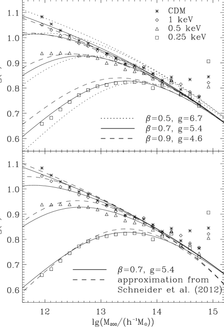
Figure 3: The dependences of concentration parameter $c$ on halo mass $M_{200}$ for different cosmologies. The data of simulations for CDM (stars) and WDM with different masses of dark matter particles ($m=1$ keV - diamonds, $m=0.5$ keV - triangles, $m=0.25$ keV - squares) are taken from r08 . Top panel: our approximation for different parameters, $\beta=0.5$, $g=6.7$ – dotted lines; $\beta=0.7$, $g=5.4$ – solid lines; and $\beta=0.9$, $g=4.6$ – dashed lines. Bottom panel: the comparison of our approximations ($\beta=0.7$, $g=5.4$, solid lines) with approximations in r08 (dashed lines).

The approximations for dependences of concentration on mass are presented in Fig. 3 for CDM and WDM (for set of DM particle masses) along with the data of simulations carried out by r08 . Also, we used the data of the simulations to find the best-fit values for the parameters, $\beta=0.7$ and $g=5.4$, and plotted them along with the approximation of same authors for comparison, see bottom panel. All calculations were performed for a number of $\Lambda$CDM and $\Lambda$WDM cosmologies with parameters $\Omega_{m}=0.2726$, $\Omega_{\Lambda}=0.7274$, $h=0.704$, $\sigma_{8}=0.809$ and $n_{s}=0.963$.

The values of halo concentrations correlate with halo ages, so that the oldest halos are expected to have larger concentrations (see r07 for details). According to hierarchical CDM scenario of clustering, the halos of lower masses should be formed in first turn, therefore they should be of larger concentrations. Meanwhile, for the WDM the perturbations at small scales are suppressed by free-streaming. As a result, in case of WDM the low-mass halos are mainly formed after cooling of warm dark matter caused by expansion of the Universe, hence they appear to have smaller values of concentration.

Another comparison of our predictions with simulations is presented in Fig. 4, this time with respect to redshift evolution. The evaluated dependence of halo concentration, $c_{200}$, on mass $M_{200}$, is presented therein along with the modeling data from b3 , the parameters of cosmological model are taken from the 5-year Data Release of WMAP b88 : $\Omega_{\Lambda}=0.721$, $\Omega_{m}=0.279$, $\Omega_{b}=0.0441$, $h=0.719$, $\sigma_{8}=0.796$ and $n_{s}=0.963$. Three plots represent dependences for the set of redshifts, $z=0,1,2$. Quite good agreement is seen between our calculations and the data of simulations at all redshifts.

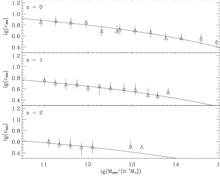
Figure 4: The dependence of concentration, $c_{200}$, on the mass $M_{200}$. The triangles represent the modeling by b3 . The solid lines represent our results. The plots are given for the redshifts $z=0,1,2$ in downward order.

IV Mass functions of halos and matter power spectrum

The pioneering paper of Press and Schechter b34 introduced an analytical approach to statistical description for galaxy clusters distribution. The model of spherical collapse underpins this formalism, the halos are associated with the peaks of an initial Gaussian field of density perturbations. This Press-Schechter formalism utilizes the halo mass function to describe the distribution of halos over masses. The approach was refined and extended afterwards in b10 ; b36 ; b37 to allow for the merger histories of dark matter halos. The process of halo merging is assumed to be hierarchical at the large scales and described with characteristic collapsing mass scale, $m(t_{col})$, complemented with r.m.s. of density perturbations, $\sigma(m)=\delta_{col}(t_{col})$. This mass grows with time through merging of halos and should asymptotically approach in distant future the limit $m_{\infty}$ at which $\sigma(m_{\infty})=\delta_{min}$, where $\delta_{min}$ is the minimal amplitude of linear density perturbations which can reach the turnaround point followed by collapse and formation of virialized objects for cosmologically justified time (see for details b17 ). For cosmology with $\delta_{min}=0$ the clustering of dark matter never ends in sense that all halos of the Universe will merge in far future.

IV.1 Halo mass function

According to b10 , the Press-Schechter mass function $n(m,z)$, i.e. the number density of gravitationally bound objects with masses $m$ at redshift $z$, is supposed to satisfy the condition

$$\nu F(\nu)\equiv\frac{m^{2}n(m,z)}{\overline{\rho}_{m}}\frac{d\ln m}{d\ln\nu}=\sqrt{\frac{\nu}{2\pi}}\exp\left\{-\nu/2\right\},$$ (39)

where $\nu\equiv(\delta_{col}(t_{col})/\sigma(m))^{2}$ and $\overline{\rho}_{m}$ is the background matter density.

The Press-Schechter mass function is proven to be qualitatively correct, however in some details the discrepancies with the data of N-body simulations are found. Therefore, the number of improvements to this approach are proposed. For instance, the treatment of the collapsing perturbations as ellipsoidal rather than spherical diminishes the discrepancies (see b38 ). Indeed, by assuming the average ellipticity of perturbation with mass $m$ and amplitude $\delta$ to be ${e}_{mp}=(\sigma(m)/\delta)/\sqrt{5}$, a simple relation was obtained in b8 to connect ellipsoidal and spherical collapse thresholds

$$\delta_{ec}(m,t_{col})=\delta_{col}(t_{col})\left(1+0.47\left[\frac{\sigma(m)}{\delta_{col}(t_{col})}\right]^{1.23}\right).$$ (40)

Also, the excursion set model was used in b10 to estimate the mass function associated with ellipsoidal collapse,

$$\nu F(\nu)=A(p)\left(1+\nu^{-p}\right)\sqrt{\frac{\nu}{2\pi}}\exp\left\{-\nu/2\right\},$$ (41)

where parameter $p\simeq 0.3$ and function $A(p)\equiv\left[1+2^{-p}\Gamma(1/2-p)/\sqrt{\pi}\right]^{-1}\simeq 0.3222$ are determined by requirement that the whole mass is gathered within halos, i.e. the integration of $F(\nu)$ over $\nu$ yields unity. In order to match the data of GIF numerical simulations the mass function (41) has been parameterized in b38 as

$$\nu F(\nu)=A(p)\left(1+(q\nu)^{-p}\right)\sqrt{\frac{q\nu}{2\pi}}\exp\left\{-q\nu/2\right\}.$$ (42)

The additional parameter $q$ was found to be $q=0.707$, later it was re-determined in b44 to be $q=0.75$. The ellipsoidal threshold for such mass function, estimated in the framework of the excursion set approach b8 , is as follows:

$$\delta_{eq}(m,t_{col})={q}^{\frac{1}{2}}\delta_{col}(t_{col})\left(1+0.5\left[\frac{\sigma(m)}{q^{\frac{1}{2}}\delta_{col}(t_{col})}\right]^{1.2}\right).$$ (43)

Two different algorithms are commonly used to identify the dark matter halos within data of numerical N-body simulations: the friend-of-friend (FOF) algorithm b39 and the spherical overdensity (SO) finder b40 . The FOF procedure depends on just one free parameter, $b$, which defines the linking length as $b\overline{n}^{-1/3}$, where $\overline{n}$ is the average density of particles. Thus, in the limit of very large number of particles per halo, FOF approximately selects the halo as matter enclosed by an isodensity surface at which $\rho=\overline{\rho}/b^{3}$. SO algorithm finds the values ​​of the average halo density in spherical volumes of various sizes. The criterion for halo identification is equality of the average density over the sphere to certain value $\kappa\overline{\rho}_{m}$, where $\overline{\rho}_{m}$ is mean density of matter in sample and $\kappa$ is a parameter of algorithm. For the NFW density profile these algorithms are not to be identical as they lead to different mass dependences of the halo concentration parameter $c$. Nevertheless, the similarity of halo mass functions was found in b41 using SO ($\kappa=180$) and FOF ($b=0.2$) halo finders.

Hereafter, we refer to halo as a gravitationally bound system which has reached the state of dynamical equilibrium, meanwhile both SO and FOF finders select the groups of close particles regardless of their dynamical properties. To divide such halos into virialized (relaxed) and non-virialized parts, it was suggested in b42 to assess the dynamical state of each halo processed by FOF algorithm by means of three objective criteria: 1) the substructure mass function $f_{sub}$, 2) the center of mass displacement $s=|r_{c}-r_{cm}|/r_{vir}$ and 3) the virial ratio $2T/U$. In b2 the r.m.s. of the NFW fit to the density profile have been used too.

As far as virial density $\rho_{vir}=\rho_{cr}\Delta_{vc}=\overline{\rho}_{m}\Delta_{vm}$, it seems appropriate to use SO halo-finder with $\kappa=\Delta_{vm}=\Delta_{vc}/\Omega_{m}$. The equality $\kappa\simeq 180$ is valid for any redshift in flat $\Omega_{m}=1$ cosmology (this is close to the $b\simeq 0.2$ for FOF algorithm), meanwhile for $\Lambda$CDM cosmology with $\Omega_{m}=0.3$, $\Omega_{\Lambda}=0.7$ the quantities $\kappa$ and $b$ depend on redshift: $\kappa\simeq 97/0.3\simeq 324$ ($b\simeq 0.164$) at $z=0$ and slowly decrease (increase) to the limit $\kappa\simeq 180$ ($b\simeq 0.2$) at high $z$. However, as it is shown in b41 , the shape of mass function is invariant if we simply identify clusters with a constant linking length, $b=0.2$, for all redshifts and cosmologies.

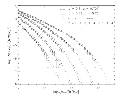
Figure 5: The halo mass function for different redshifts ($z=0,1.05,1.94,2.97,4.04$ from top to bottom). The dashed lines are Sheth-Tormen approximation with parameters $p=0.3$ and $q=0.707$ b38 , the dotted lines show the same approximation with modified parameters $p=0.32$ and $q=0.76$, diamonds show results from N-body numerical simulations performed by GIF/Virgo collaboration b46 .

The halo mass function derived from N-body simulations of GIF/Virgo collaboration is plotted in Fig. 5. The catalogs of halos were built from simulations and made available. For each halo detected by FOF-algorithm ($b=0.2$) the catalogs include the mass $M_{200}$, confined within the central part of halo with overdensity $\Delta_{vm}=200$ (see b46 for details). The mass rescaling slightly affects the ’observed’ mass function. We have re-determined the parameters of Sheth-Tormen approximation to be $p=0.32$ and $q=0.76$. As it follows from Fig. 5, the refined parameters provide a better fit for data than ones from b38 , namely $p=0.3$ and $q=0.707$. The mass function is defined here as a number density of halos with masses exceeding the specified mass $m$,

$$N(>m)=\int\limits_{m}^{\infty}n(m^{\prime},z)dm^{\prime}=\int\limits_{m}^{\infty}\frac{\overline{\rho}_{m}}{m^{\prime}}\nu F(\nu)\frac{d\ln\nu}{dm^{\prime}}dm^{\prime}.$$ (44)

Note, that variations in FOF or SO halo finder parameters also alter the total number of detected halos, meanwhile the mass rescaling influences the shape of mass function, not the total number of halos.

The Press-Schechter formalism b34 implies that halos are shaped out of regions with initial overdensities $\delta\geq\delta_{col}$, i.e. the collapsed ones. However, this does not prevent the initially lower overdensities, $\delta<\delta_{col}$, to reach the value $\Delta_{vm}$. For the non-linear overdensity $\delta_{M}=180$ the corresponding initial amplitude of density perturbation (in the units of critical one) is $q^{\frac{1}{2}}\equiv\overline{\delta}/\delta_{col}\simeq 0.95$, as it follows from (12). Thus, the SO-algorithm ($\kappa=\Delta_{vm}=\delta_{M}+1$) can by chance mark as halos the non-virialized regions, the initial amplitude of which exceeds $q^{\frac{1}{2}}\delta_{col}$ but is less than $\delta_{col}$ (for spherical overdensities).

It seems reasonable to assume that the elliptical ’q-threshold’ $\delta_{eq}$ is directly connected to spherical ’q-threshold’ $q^{\frac{1}{2}}\delta_{col}$ through (43) just in the same manner as the elliptical collapse threshold $\delta_{ec}$ is related to the spherical collapse threshold $\delta_{col}$ with (40). However, the estimate obtained above, $q\simeq 0.95^{2}\simeq 0.90$ for $\Delta_{vm}=180$, substantially deviates from $q\simeq 0.75$, estimated by numerical simulations using FOF ($b=0.2$) and SO ($\kappa=180$) algorithms. The large halos are supposed to be close to spherical, so their mass distribution should comply to Press-Schechter one. More interesting, when $\delta_{col}$ in (39) is replaced by the spherical ’q-threshold’ $0.95\delta_{col}$ ($0.9\nu$ for $\nu$), a good match to numerical simulations is attained for large $\nu$ and therefore large masses. However, the Press-Schechter mass function tends to overestimate the number of halos with smaller masses, because low-mass proto-halos are more elliptical and therefore according to (40) need larger initial amplitude to became a halo.

IV.2 The dark matter power spectrum

A luminous object is determined by clumping of baryon matter, which in turn is tightly governed by gravitational potential of dark matter. Whence, the observable spatial distribution of galaxies should follow the distribution of dark matter, since the latter dominates by density. So, in order to reconstruct the observable distribution of galaxies the characteristics of distribution of dark matter are needed.

IV.2.1 Two-point correlation function and power spectrum of discrete and continuous distributions

In statistics, the inhomogeneity of spatial distribution is usually described either by the two-point correlation function or by its Fourier transform, the power spectrum. The latter can be directly drawn by Fourier transformation of relative density fluctuations. In the case of continuous distribution it is

$$\delta(\vec{r})=(2\pi)^{\frac{3}{2}}V^{\frac{1}{2}}\int\delta_{\vec{k}}e^{-i\vec{k}\vec{r}}d^{3}\vec{k}=\frac{(2\pi)^{\frac{3}{2}}}{V^{\frac{1}{2}}}\sum\limits_{\vec{k}}\delta_{\vec{k}}e^{-i\vec{k}\vec{r}},$$ (45)

here $V$ denotes ‘volume of periodicity’ to be properly chosen. The coefficients of (45) are:

$$\delta_{\vec{k}}=\frac{1}{(2\pi)^{3/2}V^{1/2}}\int\delta(\vec{r})e^{i\vec{k}\vec{r}}d^{3}\vec{r}=\frac{V^{\frac{1}{2}}}{(2\pi)^{\frac{3}{2}}}\sum\limits_{\vec{r}}\delta(\vec{r})e^{i\vec{k}\vec{r}}.$$ (46)

The Fourier amplitude, squared and averaged over the different directions of vector $\vec{k}$, yields the power spectrum, $\mathcal{P}(k)=\left<|\delta_{\vec{k}}|^{2}\right>$. The two-point correlation function is readily derived from given power spectrum,

$$\xi(r)=\left<\delta(\vec{r}^{\prime})\delta(\vec{r}^{\prime}+\vec{r})\right>=\frac{(2\pi)^{3}}{V}\sum\limits_{\vec{k}}\left<|\delta_{\vec{k}}|^{2}\right>e^{i\vec{k}\vec{r}}$$

$$=\int d^{3}\vec{k}\left<|\delta_{\vec{k}}|^{2}\right>e^{i\vec{k}\vec{r}}=4\pi\int\limits_{0}^{\infty}k^{2}dk\mathcal{P}(k)\frac{\sin(kr)}{kr},$$ (47)

as well as variance of the amplitude within the sphere of radius $R$,

$$\sigma^{2}(R) = \left<\delta_{R}^{2}\right>=4\pi\int k^{2}\mathcal{P}(k)W^{2}(kR)dk$$ (48)

$$= \int\Delta^{2}(k)W^{2}(kR)d\ln k,$$

where $W(x)=3(\sin(x)-x\cos(x))/x^{3}$ is a window function for sphere, the quantity $\Delta^{2}(k)=4\pi k^{3}\mathcal{P}(k)$ is a “dimensionless” power spectrum.

The power spectrum is evaluated from correlation function as

$$\mathcal{P}(k)=\frac{1}{(2\pi)^{3}}\int d^{3}\vec{r}e^{-i\vec{k}\vec{r}}\xi(r).$$ (49)

The galaxy catalogs (and the data of numerical simulations) involve discrete distributions of objects (“particles”). Thus, the equations (45) and (46) should be rewritten with $\rho(\vec{r})=\sum\limits_{i}m_{i}\delta_{D}(\vec{r}-\vec{r}_{i})$, where $m_{i}$ is the mass of $i$-th particle, $\delta_{D}(\vec{r}-\vec{r}_{i})$ is three-dimensional Dirac function,

$$\delta_{\vec{k}}=\frac{1}{(2\pi)^{3/2}\left<m\right>\overline{n}V^{1/2}}\sum\limits_{i}m_{i}e^{-i\vec{k}\vec{r}_{i}},$$ (50)

$\overline{n}$ is spatially averaged number density of particles, $\left<m\right>=\sum m_{i}/(\overline{n}V)$ is the mean mass.

The relation of power spectrum to correlation function is provided in Peebles1993 , there

$$\mathcal{P}(k)=\frac{\left<m^{2}\right>}{(2\pi)^{3}\overline{n}\left<m\right>^{2}}+\frac{1}{(2\pi)^{3}}\int d^{3}\vec{r}e^{-i\vec{k}\vec{r}}\xi(r),$$ (51)

with $\left<m^{2}\right>=\sum m_{i}^{2}/(\overline{n}V)$. The first term in right-hand side is a shot noise, denoted henceforth by $\mathcal{P}_{shot}$. It is inherent for discrete distribution and caused by finiteness of the number density of particles $\overline{n}$. At $\overline{n}\to\infty$, i.e. for continuous distribution, the Eqs. (51) and (49) converge. The second term in right-hand side of (51) is denoted henceforth as $\mathcal{P}_{\xi}(k)$ to emphasize the non-random (correlated) nature of distribution. Thus, the Eq. (51) can be written in more compact form as $\mathcal{P}(k)=\mathcal{P}_{shot}+\mathcal{P}_{\xi}(k)$.

IV.2.2 Non-linear power spectrum in halo model

Within halo model the distribution of matter is treated in a mixed, discrete-continuous manner. The distribution of spatially separated halos of different mass is considered and the distribution of matter within each halo is described by continuous density profile (18). Therefore, the power spectrum is split into two terms, one to describe the distribution of halos and the second to describe the distribution of matter within individual halo. The splitting can be derived rigorously taking into account that Fourier amplitudes of density perturbations are (see for details Appendix A)

$$\delta_{\vec{k}}=\frac{1}{\overline{\rho}}\int\limits_{0}^{\infty}m\cdot n(m)\delta_{\vec{k}}(m)\overline{y}(m,k)dm.$$ (52)

The $\overline{\rho}=\overline{\rho}_{m}^{0}/a^{3}$ is an average matter density at the moment of time determined by scale factor $a=(1+z)^{-1}$ and $n(m)$ is the number density of halos with mass $m$ in comoving coordinates, estimated with (42).

The function $\overline{y}(m,k)$ is a Fourier transform of density profile (18) expressed explicitly by analytical form

$$\overline{y}(m,k)=\frac{4\pi}{m}\int\limits_{0}^{r_{vir}/a}\frac{\sin(kR)}{kR}\rho(Ra)R^{2}dR$$

$$=\frac{4\pi\rho_{s}r_{s}^{3}}{ma^{3}}\left\{\left[Si\left(\frac{kr_{s}}{a}(1+c)\right)-Si\left(\frac{kr_{s}}{a}\right)\right]\sin\left(\frac{kr_{s}}{a}\right)\right.$$

$$+\left.\left[Ci\left(\frac{kr_{s}}{a}(1+c)\right)-Ci\left(\frac{kr_{s}}{a}\right)\right]\cos\left(\frac{kr_{s}}{a}\right)\right.$$

$$-\left.\frac{a}{(1+c)kr_{s}}\sin\left(c\frac{kr_{s}}{a}\right)\right\},$$ (53)

where $c$ is the halo concentration, $\rho_{s}$ and $r_{s}$ are parameters of density profile, $Si(x)$ and $Ci(x)$ are integral sine and cosine respectively. The halo profile depends on the physical coordinates, while the power spectrum is associated with comoving coordinates as $R=r/a$. The term $4\pi\rho_{s}r_{s}^{3}/m$ can be expressed via halo concentration parameter $c$ using the Eq. (28).

The power spectrum $\mathcal{P}(k|m,m^{\prime})$ of spatial distribution of halos with given masses $m$ and $m^{\prime}$ is following:

$$\mathcal{P}(k|m,m^{\prime}) = \frac{1}{2}\left<\delta_{\vec{k}}^{*}(m)\delta_{\vec{k}}(m^{\prime})+\delta_{\vec{k}}(m)\delta_{\vec{k}}^{*}(m^{\prime})\right>$$

$$= \frac{\delta_{m,m^{\prime}}}{(2\pi)^{3}n(m)}+\mathcal{P}_{\xi}(k|m,m^{\prime}).$$

where $\delta_{m,m^{\prime}}$ is Kronecker symbol, $\mathcal{P}_{\xi}(k|m,m^{\prime})$ is Fourier image of two-point cross-correlation function of the halos, the angle brackets in the right-hand side denote the averaging over the directions of $\vec{k}$.

After the series of mathematical transformations we obtain

$$\mathcal{P}(k) = \frac{1}{(2\pi)^{3}\overline{\rho}^{2}}\int\limits_{0}^{\infty}m^{2}\cdot n(m)|\overline{y}(m,k)|^{2}dm$$

$$+ \frac{1}{\overline{\rho}^{2}}\int\limits_{0}^{\infty}m\cdot n(m)\overline{y}(m,k)dm$$

$$\times\int\limits_{0}^{\infty}m^{\prime}\cdot n(m^{\prime})\overline{y}(m^{\prime},k)dm^{\prime}\mathcal{P}_{\xi}(k|m,m^{\prime}).$$

The quantity $n(m)$ is a number density of halos of masses $m$.

Under the assumption of linearity the cross-correlation power spectrum can be represented as $\mathcal{P}_{\xi}(k|m,m^{\prime})\approx b(m)b(m^{\prime})\mathcal{P}_{lin}(k)$, $\mathcal{P}_{lin}(k)$ is the linear power spectrum of spatial distribution of matter, $b(m)$ is the biasing parameter which characterizes the skew between distributions of halos and matter.

The requirement of homogeneity at largest scales imposes that expression (IV.2.2) has to asymptotically approach zero for small wave numbers $k$. Nevertheless, the first term in right-hand side of (IV.2.2) never diminishes, because the binning of matter into separate halos (a kind of discretization) introduces the noise into the procedure. The expression for noise is derived from the first term in (IV.2.2) by letting the distribution of halo matter to be homogeneous and substituting of Fourier image of profile $\overline{y}(k,m)$ by window function $W(kR)$, where $R=(3m/(4\pi\overline{\rho}_{m}))^{1/3}$. After noise elimination the final expression for the power spectrum of spatial distribution of dark matter is following:

$$\!\!\!\!\!\!\!\!\!\!\!\!\!\mathcal{P}(k)=\frac{1}{(2\pi)^{3}}\int\limits_{0}^{\infty}\left(\frac{m}{\overline{\rho}}\right)^{2}n(m)\left[|\overline{y}(m,k)|^{2}-W^{2}(kR)\right]dm$$

$$\,+\left[\int\limits_{0}^{\infty}\frac{m}{\overline{\rho}}b_{1}(m)n(m)\overline{y}(m,k)dm\right]^{2}\mathcal{P}_{lin}(k).$$ (55)

In accordance with r10 the factor $[|\overline{y}(m,k)|^{2}-W^{2}(kR)]$ is used instead of $[\overline{y}(m,k)-W(kR)]^{2}$, as mentioned in the review b0 on the halo model. It should be stressed, that at quasilinear stage it yields rather small deviations from the numerical simulation because $[|\overline{y}(m,k)|^{2}-W^{2}(kR)]\geq[\overline{y}(m,k)-W(kR)]^{2}$ at $k\sim 1/R$.

Table 1: The parameters of Large Box (LB) and GIF2 simulations, available from Max Planck Institute for Astrophysics in Garching (http://www.mpa-garching.mpg.de).

Simul.	Npar	L (Mpc/h)	$m_{p}$ ($M_{sun}$/h)	$l_{soft}$ (Kpc/h)
GIF2	4003	110.0	1.73$\times 10^{9}$	6.6
LB	5123	479.0	6.86$\times 10^{10}$	30

With Eq. (55) the power spectrum of dark matter is computed for the broad range of scales to confront our estimations with results of Large Box and GIF2 N-body simulations available from Max Planck Institute for Astrophysics in Garching. The results of simulation are released as files with coordinates, velocities and identification numbers of particles. The parameters of simulations, namely the total number of particles, the size of box, the mass of particles (assumed equal for all particles) and the scale of smoothing are presented in the Tab. 1. The latter is introduced in order to eliminate numerical singularities due to particles proximity, when floating-point errors are difficult to control.

To reproduce the structure at small scales a simulation should engage the high number density of particles. On the other hand, large volume is required to reproduce properly the structure at large scales. A pursuit to simultaneously meet both requirements leads to the huge numbers of particles and consequently to the enormous amount of computational efforts. So, the commonly used trick is to run separate simulations for largest and smallest scales. Whence, the Large Box simulations cover large volumes, whereas the the GIF2 simulations provide us with data for small scales with larger number density of particles.

Figure 6: Dark matter power spectrum from LB (asterisk) and GIF2 (diamonds) simulations. Solid lines represent the primordial linear power spectrum from b49 (lower line) and our predictions for non-linear one (upper line). Dash-dotted lines show the ’halo-halo’ and the ’shot noise’ components. Dotted and dashed lines represent PD96 b15 and HALOFIT b14 approximations respectively. The parameters of $\Lambda$CDM model here are as follows: ($\Omega_{m}$, $\Omega_{\Lambda}$, $h$, $\sigma_{8}$, $n_{s}$)=(0.3, 0.7, 0.7, 0.9, 1).

The power spectrum was evaluated by computation of the sums, $Sr(\vec{k})=\sum_{i}\cos(\vec{k}\vec{r}_{i})$ and $Si(\vec{k})=\sum_{i}\sin(\vec{k}\vec{r}_{i})$, followed by overall summation, $\mathcal{P}(\vec{k})=(Sr^{2}(\vec{k})+Si^{2}(\vec{k}))/((2\pi)^{3}\overline{n}^{2}V)$. The final power spectrum was estimated by averaging over directions of $\vec{k}$. To eliminate the noise, the power spectrum of homogeneous distribution was computed in advance and substracted later from the total power spectrum.

In Fig. 6 the results are presented for different techniques. The dark matter power spectrum predicted by our halo model, Eq. (55), apparently matches the LB/GIF2 non-linear power spectrum through all scales up to $k\sim 100$ h/Mpc. Also, the PD96 b15 and HALOFIT b14 approximations are plotted therein, based on the halo model of Hamilton et al. Hamilton1991 , as well as scaling relations and fits to numerical simulations. All these approximations appear to properly fit the LB/GIF2 non-linear power spectrum at the whole range of scales. The linear power spectrum was evaluated by analytical approximation from b49 (lower solid line in Fig. 6) and normalized to $\sigma_{8}=0.9$.

Since the non-linear corrections are not essential at $k\leq 0.2$ h/Mpc, the power spectrum appears to be linear there (Fig. 6). The non-linear clustering enhances the power spectrum at smaller scales, $k>0.2$ h/Mpc. Both approximations, our (55) and HALOFIT, reproduce such behavior appropriately. Consistency of our estimation with numerical simulations data and HALOFIT approximation proves the plausibility of our approach.

The halo mass function in WDM cosmology is expected to decline at low masses as $n_{h}(m)=(1+m_{hm}/m)^{-0.6}n_{ST}(m)$ r08 , where $n_{ST}(m)$ denotes the Sheth-Tormen mass function described in section IV.1. The WDM tends to clump less, so that contributes largely to a smooth component of density field, $\rho_{s}$, with $\overline{\rho}=\overline{\rho}_{h}+\overline{\rho}_{s}$ r11 ; r08 . To treat the WDM within the framework of halo model the separate particles of dark matter are considered as point halos with mass $m_{DM}$, immersed into smooth component. Thus, the total number density of halos is

$$n(m)=n_{h}(m)+\frac{\overline{\rho}_{s}}{m_{DM}}\delta_{D}(m-m_{DM}).$$ (56)

With substitution to (55), similarly to r11 , the power spectrum

$$\!\!\!\!\!\!\!\!\!\!\!\!\!\mathcal{P}(k)=\frac{1}{(2\pi)^{3}}\int\limits_{0}^{\infty}\left(\frac{m}{\overline{\rho}}\right)^{2}n_{h}(m)\left[|\overline{y}(m,k)|^{2}-W^{2}(kR)\right]dm$$

$$\,+\left[\int\limits_{0}^{\infty}\frac{m}{\overline{\rho}}b_{1}(m)n_{h}(m)\overline{y}(m,k)dm+b_{s}\frac{\overline{\rho}_{s}}{\overline{\rho}}\right]^{2}\mathcal{P}_{lin}(k).$$

where biasing factor of smooth component can be obtained from

$$b_{s}\frac{\overline{\rho}_{s}}{\overline{\rho}}=1-\int\limits_{0}^{\infty}\frac{m}{\overline{\rho}}b_{1}(m)n_{h}(m)dm.$$

Figure 7: The difference (per cent) between non-linear power spectra of $\Lambda$CDM and $\Lambda$WDM models with ($\Omega_{m}$, $\Omega_{\Lambda}$, $\Omega_{b}$, $h$, $n_{s}$, $\sigma_{8}$)=(0.2711, 0.7289, 0.0451, 0.703, 0.966, 0.809) and two values of WDM particle mass: $m_{wdm}=1$ keV and $m_{wdm}=0.5$ keV.

The applicability of these formulas was verified by comparison with the results of numerical simulations from b100 . The initial distribution of warm dark matter particles for simulation was generated by following linear power spectrum:

$$\mathcal{P}_{lin}^{(wdm)}(k)=\mathcal{P}_{lin}^{(cdm)}(k)\left[\left(1+(\alpha k)^{2\nu}\right)^{-5/\nu}\right]^{2},$$ (57)

with $\nu=1.12$. The parameter $\alpha$ (in units of Mpc/h) depends on the mass of WDM particles $m_{wdm}$, their density $\Omega_{wdm}$ and Hubble parameter as

$$\alpha(m_{wdm})=0.049\left(\frac{1keV}{m_{wdm}}\right)^{1.11}\left(\frac{\Omega_{wdm}}{0.25}\right)^{0.11}\left(\frac{h}{0.7}\right)^{1.22}$$

(see also Hansen2002 and Viel2005 ).

The non-linear power spectrum of matter density perturbations at $z$ = 0.5 was evaluated by (55) for $\Lambda$CDM and $\Lambda$WDM cosmologies with parameters set ($\Omega_{m}$, $\Omega_{\Lambda}$, $\Omega_{b}$, $h$, $n_{s}$, $\sigma_{8}$)=(0.2711, 0.7289, 0.0451, 0.703, 0.966, 0.809) and two masses of warm dark matter particles, $m_{wdm}$, 1 and 0.5 keV, the same as in b100 . The Fig. 7 represents the relative discrepancies (percentage) between non-linear power spectra of cold and warm dark matter (solid lines), also the corresponding spectra from simulations are plotted along (Fig. 7 in b100 ). Our results reveal qualitative consistency with simulations however quantitative differences are still noticeable.

It is worth to mention the discrepancy of halo model and numerical simulations in case of warm dark matter Smith2011 , see the bottom panels of Figure 7 in paper b100 (green line). That estimation appears to be suppressed in comparison with numerical simulation and seems to be closer to our results. The plausible explanation is that the low-mass halos are more clustered in WDM models than in CDM ones. As it was noted in r12 , “formation of low mass halos almost solely withing caustic pancakes or ribbons connecting larger halos in a ’cosmic web’ ”, and “voids in this web are almost empty of small halos, in contrast to the situation in CDM theory”. This leads to larger values of biasing at $m<m_{hm}$ in WDM models with respect to CDM r08 . We assume that the reason why small halos with mass below $m_{hm}$ are so strongly clustered is that they belong (at least partially) to some larger halos (i.e. they are satellites). Dashed lines in Fig. 7 represent the computations for the case when masses of all halos are increased by 4%, to be above $m_{hm}$.

Note some aspects of the problem to be addressed in further studies:

• The halos with mass $<m_{hm}$ can appear in result of: i) tidal stripping of dark matter from initially more massive halos, ii) evaporation of subhalos from large mass halos and iii) clustering in cold component of dark matter. Clarification of the contribution of each of such mechanisms is needed to update properly the halo model.

• When the power spectra were calculated, the variance of the parameter of halo concentration $\sigma_{\ln c}=0.25$ was assumed to be the same for the cold and warm dark matter and independent of the halo mass. It follows from Fig. 7, that the deviations can be caused by the halo concentration variations.

• Halo model by itself has a number of problems and not to be considered as ultimately accurate. It is based on some strong assumptions, contains a series of approximations and uncertain statistical procedures, thus prone to systematic errors.

IV.3 The galaxy power spectrum

As the baryon gas falls into potential wells of virialized dark matter halos and subhalos it is heated up to virial temperature of $T=\frac{1}{2}\mu m_{p}v_{vir}^{2}/k_{B}\approx 2\times 10^{4}\mu_{0.6}(M/10^{8}M_{\odot})^{2/3}[(1+z)/10]$ K, where $\mu=0.6\mu_{0.6}$ is the mean molecular mass of post-shock gas and $M$ is the mass of halo or subhalo progenitors. The temperature of baryon matter gradually decreases afterwards due to the cooling processes (see b4 ). It results in fragmentation to smaller clumps with Bonnor-Ebert mass, $M_{BE}\simeq 700M_{\odot}(T/200\textrm{K})^{3/2}(n_{b}/10^{4}\textrm{cm}^{-3})^{-1/2}$, where $n_{b}$ is the total number density of baryon particles. At the final stage of this fragmentation the stars and galaxies are formed (see b4 and b6 for details). Since formation of galaxies is driven by gravity of dark matter, the spatial distribution of galaxies should track the spatial distribution of dark matter. In other words, the fluctuations of dark matter density $\delta_{DM}(\vec{r})=\rho_{DM}(\vec{r})/\overline{\rho}_{DM}-1$ correlate with fluctuations of galaxy number density $\delta_{g}(\vec{r})=n_{g}(\vec{r})/\overline{n}_{g}-1$.

In halo model, the galaxy number density fluctuations have the following Fourier amplitude:

$$\delta_{g|\vec{k}}\;=\frac{1}{\overline{n}_{g}}\int\limits_{m_{min}}^{\infty}\left<N_{g}|m\right>n(m)\delta_{\vec{k}}(m)\overline{y}_{g}(k,m)dm$$ (58)

(see Appendix B for details ). Here $\left<N_{g}|m\right>$ is a mean number of galaxies in halo with mass $m$, $\overline{y}_{g}(k,m)$ is a Fourier transform of galaxy number density profile and $m_{min}$ denotes the lowest limit for halo mass below which no galaxies are formed. Such limit naturally stems from degrading efficiency of star formation in halos of low mass b1 and conditions imposed on the sample of galaxies (see b26 ; b27 ).

The considerations of previous subsection are summarized in the following galaxy power spectrum:

$$\!\!\!\!\!\!\!\!\!\!\!\!\!\mathcal{P}_{g}(k)=\frac{1}{(2\pi)^{3}}\int\limits_{m_{min}}^{\infty}\left(\frac{\left<N_{g}|m\right>}{\overline{n}_{g}}\right)^{2}n(m)$$

$$\!\!\!\!\!\!\!\!\!\!\times\left[|\overline{y}_{g}(m,k)|^{2}-W^{2}(kR_{g})\right]dm$$ (59)

$$\!\!\!\!\!\!\!\!\!\!+\left[\int\limits_{m_{min}}^{\infty}\frac{\left<N_{g}|m\right>}{\overline{n}_{g}}b_{1}(m)n(m)\overline{y}_{g}(m,k)dm\right]^{2}\mathcal{P}_{lin}(k),$$

where $R_{g}=(3\left<N_{g}|m\right>/(4\pi\overline{n}_{g}))^{1/3}$. The resulting equation is similar to the corresponding expression for the galaxy power spectrum from b0 . The difference is caused by elimination of the noise as described above. Also, the term ${\left<N_{g}|m\right>}^{2}$ has been obtained instead of $\left<N_{g}(N_{g}-1)|m\right>$ in b0 . For large-mass halos the term $\left<N_{g}|m\right>$ is large, and it seems appropriate to assume the probability distribution $p(N_{g}|m)$ to be one of Poisson. In this case ${\left<N_{g}|m\right>}^{2}\approx\left<N_{g}(N_{g}-1)|m\right>$. However, such approximation is not valid for low-mass halos.

As it has been outlined in b20 , galaxies within halo usually are disposed around the center (central galaxy) and within each of its subhalos (satellite galaxies). This gives a clue how to find out the distribution of galaxies over the halo and how it is connected to the substructure. Massive halos usually undergo the violent relaxation, so the resulting velocity dispersion does not depend on masses of particles or subhalos. Therefore for the number density of the satellites within halo the following equation is appropriate:

$$\!\!\!\!\!\!\!\!\!\!\!\!\!n_{sg}(r)=\sum_{m\geq m^{\prime}_{min}}\!\!\!\!\!n_{sh}(m,r)=\sum_{m\geq m^{\prime}_{min}}\!\!\!\!\!n_{0}(m)\exp\left\{-\frac{m\Phi(r)}{kT}\right\}$$

$$\;\,=n_{g}^{0}\exp\left\{-\frac{3\Phi(r)}{\sigma_{v}^{2}}\right\}=\frac{n_{g}^{0}}{\rho_{s}}\rho(r),$$ (60)

where $n_{sh}(m,r)$ denotes the dependence of the number density of halo particles (subhalos) of mass $m$ on the radial distance.

As above, we assume that galaxies are formed within subhalos with masses $m\geq m^{\prime}_{min}$, where $m^{\prime}_{min}$ is less than $m_{min}$ because subhalos usually lose the mass due to tidal deprivation of their outskirts. Baryon matter (stars) is concentrated to the center and more tightly bound, meanwhile dark matter is stripped off. Thus, a subhalo at the time of observation is apparently a poor tracer of potential well, which still determines galaxy properties such as stellar mass or luminosity. A better tracer is the subhalo mass at the time when it falls into the host halo or its maximal mass over its history r20 ; b20 . For massive halos with numerous satellites the presence of the central galaxy can be neglected. In such case, as follows from (60), the assumption $\overline{y}_{g}(m,k)\simeq\overline{y}(m,k)$ is correct. This result agrees with b102 , there the spatial distribution of satellites is studied using SDSS spectroscopic and photometric galaxy catalogs. They found that satellite profiles generally have a universal form well-fitted by NFW approximation.

However, as long as low-mass halos possess a small number of galaxies, slow relaxation can be important as well. In result, the profile of satellite galaxy number density generally deviates from the profile of dark matter density. However, such discrepancy is difficult to detect because of large statistical uncertainties in determination of the profile of the galaxy number density in such halos. Let us note that in this case the presence of central galaxy could not be discarded.

Figure 8: The power spectra of galaxies (solid line) and dark matter (dotted line) calculated in halo model for $\Lambda$CDM cosmology with ($\Omega_{m}$, $\Omega_{\Lambda}$, $h$, $\sigma_{8}$, $n_{s}$) = (0.26, 0.74, 0.72, 0.77, 0.95). The squares and triangles represent the observed galaxy power spectrum from PSCz b26 and SDSS b27 galaxy catalogs respectively.

The spatial number density of the galaxies is a sum of the halo and subhalo number densities: $n_{g}(\vec{r})=n_{h}(\vec{r})+n_{sh}(\vec{r})$. The spatial fluctuation of galaxy number density can be thereby split into fluctuations of halo and subhalo numbers densities:

$$\delta_{g}(\vec{r}) = \frac{n_{h}(\vec{r})+n_{sh}(\vec{r})}{\overline{n}_{h}+\overline{n}_{sh}}-1$$ (61)

$$= \frac{1}{\overline{n}_{h}+\overline{n}_{sh}}\left[\overline{n}_{h}\delta_{h}(\vec{r})+\overline{n}_{sh}\delta_{sh}(\vec{r})\right],$$

where as before the overlines denote averaging in space. Corresponding Fourier amplitude takes the form

$$\!\!\!\!\!\!\!\!\!\!\!\!\!\delta_{g|\vec{k}}=\frac{1}{\overline{n}_{h}+\overline{n}_{sh}}\left[\overline{n}_{h}\delta_{h|\vec{k}}+\overline{n}_{sh}\delta_{sh|\vec{k}}\right]$$ (62)

$$\!\!\!\!\!\!\!\!\!\!\!\!\!=\frac{1}{\overline{n}_{h}+\overline{n}_{sh}}\int\limits_{m_{min}}^{\infty}\!\!\!\!\!\left[1+\left<N_{sh}|m\right>\overline{y}_{sh}(k,m)\right]n(m)\delta_{\vec{k}}(m)dm,$$

where $\left<N_{sh}|m\right>$ is the average number of subhalos confined within the halo of mass $m$, virtually the number of satellites. Since the average number of galaxies accounts for central galaxy and satellites, $\left<N_{g}|m\right>=1+\left<N_{sh}|m\right>$. By comparing Eqs. (58) and (62) one can obtains

$$\overline{n}_{g}=\overline{n}_{h}+\overline{n}_{sh}=\int\limits_{m_{min}}^{\infty}\!\!\!\!\!\left[1+\left<N_{sh}|m\right>\right]n(m)dm,$$

and

$$\overline{y}_{g}(k,m)=\frac{\left<N_{sh}|m\right>\overline{y}_{sh}(k,m)+\overline{y}_{c}(k,m)}{\left<N_{sh}|m\right>+1},$$

where $\overline{y}_{sh}(k,m)$ is a Fourier image of the subhalo number density profile, meanwhile $\overline{y}_{c}(k,m)$ is a Fourier image of the probability of finding the central galaxy within the halo.

In cases of strictly central location of ‘core’ galaxies in all halos with masses $m$ $\overline{y}_{c}(k,m)=1$. For massive halo, $\left<N_{sh}|m\right>\gg 1$, so $\overline{y}_{g}(k,m)\simeq\overline{y}_{sh}(k,m)$, whereas for low-mass halo, $\left<N_{sh}|m\right>\ll 1$, $\overline{y}_{g}(k,m)\simeq\overline{y}_{c}(k,m)$. As follows from Eq. (60) for massive halos we can assume $\overline{y}_{sh}(k,m)\simeq\overline{y}(k,m)$. For simplicity, let us extend this approximation to the case of low-mass halo. It should not bring significant errors to $\overline{y}_{g}(k,m)$ because in the case of $\left<N_{sh}|m\right>\ll 1$ the core galaxy is dominating, so $\overline{y}_{g}(k,m)\simeq\overline{y}_{c}(k,m)$.

To specify the dependence $\left<N_{sh}|m\right>$ and to provide a direct link to the galaxy sample the CLF b19 ; b32 ; b33 or CMF b20 ) can be used. The CLF, $\Phi(L|m)dL$, yields the average number of galaxies with luminosity $L\pm dL/2$ which reside within a halo of mass $m$. The CMF, $\Phi(m_{*}|m)dm_{*}$, yields the average number of galaxies with stellar masses in the range $m_{*}\pm dm_{*}/2$ which reside within halo of mass $m$. The CMF (as well as CLF) can be split into central (core) and satellite parts so that $\Phi(m_{*}|m)=\Phi_{s}(m_{*}|m)+\Phi_{c}(m_{*}|m)$. This allows us to calculate the average number of satellites with a stellar masses exceeding $m_{*}$ within the halo with mass $m$ (see b20 for details),

$$\left<N_{sh}|m,m_{*}\right>=\int\limits^{\infty}_{m_{*}}\Phi_{s}(m_{*}^{\prime}|m)dm_{*}^{\prime},$$

and the probability of finding the appropriate central galaxy is

$$\left<N_{c}|m,m_{*}\right>=\int\limits^{\infty}_{m_{*}}\Phi_{c}(m_{*}^{\prime}|m)dm_{*}^{\prime},$$

where upper limit is assigned to infinity, although it actually does not exceed the halo mass $m$. To calculate the power spectrum of galaxies, we assume that $\left<N_{g}|m\right>=\left<N_{sh}|m,m_{*}\right>+\left<N_{c}|m,m_{*}\right>$ and

$$\overline{y}_{g}(k,m)=\frac{\left<N_{sh}|m,m^{*}\right>\overline{y}_{sh}(k,m)+\left<N_{c}|m,m^{*}\right>\overline{y}_{c}(k,m)}{\left<N_{sh}|m,m^{*}\right>+\left<N_{c}|m,m^{*}\right>}.$$ (63)

The average number of galaxies with a stellar mass larger than $m_{*}$ is given by

$$\overline{n}_{g}=\int\limits_{0}^{\infty}\left[\left<N_{sh}|m,m_{*}\right>+\left<N_{c}|m,m_{*}\right>\right]n(m)dm.$$ (64)

The similar calculations are valid for CLF. Hence, the halo model describes the connection between galaxy power spectrum and stellar masses or luminosities of the sample of galaxies.

Note that our approach differs from the one proposed in b0 since it allows to consider the displacements of position of central galaxy in halos. This is important for small mass halos which tend to have large ellipticity and shallow potential wells. So, we predict that halos which contain single galaxy give contribution to the 1st term of galaxy power spectrum (59), also called as 1-halo term.

To prove our approach, we calculate the galaxy power spectrum along with error bars using the CMF from b20 for $\Lambda$CDM cosmology with parameters ($\Omega_{m}$, $\Omega_{\Lambda}$, $h$, $\sigma_{8}$, $n_{s}$) = ($0.26$, $0.74$, $0.72$, $0.77$, $0.95$). The initial dark matter power spectrum, $\mathcal{P}_{lin}(k)$, was computed with the CAMB code camb ; camb_source for $\Omega_{b}=0.05$. The galaxy power spectrum was evaluated by the Eq. (63) and Eq. (59) with $W(kR_{g})$ replaced by

$$\lim_{\mathcal{P}(k)\rightarrow 0}\overline{y}_{g}(k,m)=$$

$$\frac{\left<N_{sh}|m,m^{*}\right>W(kR_{s})+\left<N_{c}|m,m^{*}\right>W(kR_{c})}{\left<N_{sh}|m,m^{*}\right>+\left<N_{c}|m,m^{*}\right>},$$

where $R_{s}=\left(3\left<N_{sh}|m,m^{*}\right>/(4\pi\overline{n}_{g})\right)^{1/3}$ and $R_{c}=(3\left<N_{c}|m,m^{*}\right>/(4\pi\overline{n}_{g}))^{1/3}$. Also, it is assumed

$$\overline{y}_{sh}(k,m)=\int\limits_{allc}\overline{y}(k,r_{s},c^{\prime})p(c^{\prime}|m,z)dc^{\prime}.$$ (65)

where $\overline{y}(k,r_{s},c)$ denotes the dependence (53) and $p(c|m,z)$ is the probability distribution function for concentration (19) with variance $\sigma_{\ln c}=0.25$.

The obtained galaxy and dark matter power spectra are presented in Fig. 8 along with observed galaxy power spectra from PSCz b26 and SDSS b27 galaxy catalogs.

The upper solid line represents the assumption that the core galaxies in all halos with masses $m$ are located strictly in their centers, so $\overline{y}_{c}(k,m)=1$. The lower solid line represents the result for assumption that central galaxies are homogeneously distributed over the spherical volume of radius $1.1r_{s}$, so $\overline{y}_{c}(k,m)=W(1.1r_{s}k)$. We define the lower limit on the stellar masses of the galaxies to be $m_{*}=5\times 10^{6}$ $M_{\odot}$.

Thus, at large scales, $k\leq 1$ h/Mpc, the dark matter and galaxy power spectra coincide, at galaxy cluster scales, $1\leq k\leq 20$ h/Mpc, they are close and start to diverge at smaller scales, $k>20$ h/Mpc, where luminous matter is substantially more clustered than dark matter.

V Conclusions

The presented semi-analytical treatment is our implementation of halo model and it is proven to be correct in describing and interpretation of the clustering of the matter at the non-linear stage of evolution, both in simulated and observed Universe. Some of basic elements of theory are reviewed and improved to calculate the dark matter and galaxy power spectra.

A new technique is proposed for calculating halo concentration parameter, $c$, with phenomenology of halo merging, density profiles and statistical properties taken into account. The simple expression for estimation (36) depends on the relation of the halo overdensity, $\Delta_{hc}$ or $\Delta_{hm}$, and corresponding characteristic halo overdensity, $\Delta_{sc}$ or $\Delta_{sm}$ respectively. This relation is evaluated without computing redshift of halo collapse, $z_{col}$, by set of equations: (36), (31), (33), (16) and (37) or (38) as well. Such technique has been applied to calculate the concentration parameter for $\Lambda$CDM and $\Lambda$WDM cosmological models and the concordance with data of simulations b5 ; b3 for vast range of halo masses (Figs. 3, 4) has been revealed.

The parameters of Sheth-Tormen approximation for halo mass function were re-evaluated as $p=0.32$ and $q=0.76$ (see Fig. 5) to provide best-fit to the data of GIF/Virgo N-body simulations b46 (see Fig. 5).

This modified and extended halo model enables to predict the dark matter and galaxy power spectra at small scales up to $k\sim 100$ h/Mpc by means of semi-analytical methods: Eqs. (IV.2.2), (55), (59). The estimated spectra agree with non-linear power spectra determined from Large Box and GIF2 N-body simulations (Fig. 6) as well as with estimations by galaxy catalogs PSCz b26 and SDSS b27 (Fig. 8). Moreover, with the assumption on presence of the central galaxies in all halos with masses $m$ ($\overline{y}_{c}(k,m)=1$) the technique predicts galaxy power spectrum matching well the observational one up to $k\sim 20$ h/Mpc. Meanwhile, when non-central position of most massive galaxies in halos is assumed, ($\overline{y}_{c}(k,m)=W(1.1r_{s}k)$), the predictions agree with the observational data up to $k\sim 80$ h/Mpc.

The calculated non-linear galaxy power spectrum for $\Lambda$CDM cosmology with ($\Omega_{m}$, $\Omega_{\Lambda}$, $h$, $\sigma_{8}$, $n_{s}$) = (0.26, 0.74, 0.72, 0.77, 0.95) corresponds to the observational one for lower limitation on the stellar masses of the galaxies $m_{*}=5\cdot 10^{6}$ $M_{\odot}$. To attain the same level of agreement of the predicted galaxy power spectrum with extracted from galaxy surveys at smaller scales ($k>80$ h/Mpc), a new, much more complicated approach for the formation of groups of galaxies should be elaborated.

Despite the ambiguities in the definition of halo, determining of their mass, concentration and substructure, halo model provides a good reproduction of such characteristics of large-scale structure of the Universe as the power spectrum and correlation function of the spatial distribution of dark matter and galaxies. In this paper we have shown how relation between statistics of the dark matter clustering obtained from numerical simulations and galaxy statistics obtained from large galaxy surveys allows to calculate the power spectrum of the spatial distribution of the galaxies.

Appendix A Fourier modes of dark matter density inhomogeneities

The power spectrum can be derived in more rigorous manner by the series of following mathematical transformations:

$$\delta_{\vec{k}}=\frac{1}{(2\pi)^{\frac{3}{2}}V^{\frac{1}{2}}}\int\limits_{V}\delta(\vec{r})e^{i\vec{k}\vec{r}}d^{3}\vec{r}=\frac{1}{(2\pi)^{\frac{3}{2}}V^{\frac{1}{2}}}\sum\limits_{i}e^{i\vec{k}\vec{r}_{i}}\int\limits_{V_{i}}\frac{\rho(\vec{r}-{\vec{r}}_{i})}{\overline{\rho}}e^{i\vec{k}(\vec{r}-{\vec{r}}_{i})}d^{3}(\vec{r}-{\vec{r}}_{i})$$

$$=\frac{1}{(2\pi)^{\frac{3}{2}}\overline{\rho}V^{\frac{1}{2}}}\sum\limits_{i}e^{i\vec{k}\vec{r}_{i}}m_{i}\left\{\frac{1}{m_{i}}\int\limits_{V_{i}}\rho(\vec{r}-{\vec{r}}_{i})e^{i\vec{k}(\vec{r}-{\vec{r}}_{i})}d^{3}(\vec{r}-{\vec{r}}_{i})\right\}=\frac{1}{(2\pi)^{\frac{3}{2}}\overline{\rho}V^{\frac{1}{2}}}\sum\limits_{i}e^{i\vec{k}{\vec{r}}_{i}}m_{i}y_{i}(k)$$

$$=\frac{1}{\overline{\rho}}\sum\limits_{j}n(m_{j})m_{j}\left\{\frac{1}{(2\pi)^{\frac{3}{2}}V^{\frac{1}{2}}n(m_{j})}\sum\limits_{l=1}^{N_{j}}e^{i\vec{k}{\vec{r}}_{l}}y_{l}(k,m_{j})\right\}=\frac{1}{\overline{\rho}}\int\limits_{0}^{\infty}m\cdot n(m)\delta_{\vec{k}}(m)\overline{y}(m,k)dm$$

Here, the integration over the whole volume $V$ has been split into integrations over volumes $V_{i}$, each occupied by spatially separated halos; the Fourier transform of $i$-th density profile we denote as $y_{i}(k)$, it is normalized by its masses $m_{i}$. The halos are binned into the subsets with equal masses $m_{j}$, the number of halos is denoted by $N_{j}$. Also, it was assumed that the halos of equal masses have identical density profiles and, correspondingly, their Fourier transforms, $\overline{y}(m,k)$, are identical too. The $\delta_{\vec{k}}(m)$ is denotation of Fourier amplitude of spatial distribution of halos with masses $m$. The summation has been changed to the integration.

Appendix B Fourier modes of galaxy number density inhomogeneities

The Fourier amplitude for relative fluctuations of galaxy concentration takes the following form:

$$\delta_{g|\vec{k}}=\frac{1}{(2\pi)^{\frac{3}{2}}V^{\frac{1}{2}}}\int\limits_{V}\delta_{g}(\vec{r})e^{i\vec{k}\vec{r}}d^{3}\vec{r}$$

$$=\frac{1}{(2\pi)^{\frac{3}{2}}V^{\frac{1}{2}}}\sum\limits_{i}e^{i\vec{k}\vec{r}_{i}}\int\limits_{V_{i}}\frac{n_{g}(\vec{r}-{\vec{r}}_{i})}{\overline{n}_{g}}e^{i\vec{k}(\vec{r}-{\vec{r}}_{i})}d^{3}(\vec{r}-{\vec{r}}_{i})=\frac{1}{(2\pi)^{\frac{3}{2}}\overline{n}_{g}V^{\frac{1}{2}}}\sum\limits_{i}e^{i\vec{k}\vec{r}_{i}}N_{g|i}\left\{\frac{1}{N_{g|i}}\int\limits_{V_{i}}n_{g}(\vec{r}-{\vec{r}}_{i})e^{i\vec{k}(\vec{r}-{\vec{r}}_{i})}d^{3}(\vec{r}-{\vec{r}}_{i})\right\}$$

$$=\frac{1}{(2\pi)^{\frac{3}{2}}\overline{n}_{g}V^{\frac{1}{2}}}\sum\limits_{i}e^{i\vec{k}{\vec{r}}_{i}}N_{g|i}y_{g|i}(k)=\frac{1}{(2\pi)^{\frac{3}{2}}\overline{n}_{g}V^{\frac{1}{2}}}\sum\limits_{m}\sum\limits_{j_{m}}e^{i\vec{k}{\vec{r}}_{j_{m}}}N_{g|j_{m}}y_{g|j_{m}}(k,m)$$

$$=\frac{1}{\overline{n}_{g}}\sum\limits_{m}\overline{y}_{g}(k,m)\left\{\frac{1}{(2\pi)^{\frac{3}{2}}V^{\frac{1}{2}}}\sum_{j_{m}}N_{g|j_{m}}e^{i\vec{k}{\vec{r}}_{j_{m}}}\right\}=\frac{1}{\overline{n}_{g}}\sum\limits_{m}\overline{y}_{g}(k,m)\sum\limits_{N=0}^{\infty}Nn(m,N)\left\{\frac{1}{(2\pi)^{\frac{3}{2}}V^{\frac{1}{2}}n(m,N)}\sum_{l_{mN}}e^{i\vec{k}{\vec{r}}_{l_{mN}}}\right\}$$

$$=\frac{1}{\overline{n}_{g}}\sum\limits_{m}\overline{y}_{g}(k,m)\sum\limits_{N=0}^{\infty}Nn(m)p(N|m)\delta_{\vec{k}}(m,N)=\frac{1}{\overline{n}_{g}}\sum\limits_{m}n(m)\delta_{\vec{k}}(m)\overline{y}_{g}(k,m)\sum\limits_{N=0}^{\infty}Np(N|m)$$

$$=\frac{1}{\overline{n}_{g}}\int\limits_{0}^{\infty}\left<N|m\right>n(m)\delta_{\vec{k}}(m)\overline{y}_{g}(k,m)dm,$$

Here, as in Appendix A, the integration over whole volume $V$ was replaced by integration over the number of volumes $V_{i}$, filled by spatially separated halos. The Fourier images of profiles of concentration of galaxies in halo are normalized by their number $N_{g|i}$; the Fourier image of $i$-th profile of galaxy concentration is denoted by $y_{g|i}(k)$. The halo was partitioned into subsets of equal masses $m$ and normalized by means of index $j_{m}$.

It was assumed that halo of equal masses have identical profiles of galaxy concentration, so their Fourier images $\overline{y}_{g}(m,k)$ are identical; the sets of halos with equal masses $m$ were partitioned into subsets containing the same number $N$ of galaxies and denoted as $n(m,N)$. The halo concentration $n(m,N)$ is represented as a product of concentration of all halos with mass $m$ and conditional probability of event that these halos contain $N$ galaxies each, $n(m,N)=n(m)p(N|m)$. The designation was introduced for Fourier amplitude of spatial distribution of halos with masses $m$ and containing $N$ galaxies as $\delta_{\vec{k}}(m,N)$. It was assumed that spatial distribution of halos of mass $m$ and number of galaxies $N$ match the spatial distribution of all halos with masses $m$, $\delta_{\vec{k}}(m)=\delta_{\vec{k}}(m,N)$. The average number of galaxies in halo of mass $m$ is denoted as $\left<N|m\right>=\sum\limits_{N=0}^{\infty}Np(N|m)$, also the sum was replaced by integration.

References

- (1) S.D.M. White, M. Rees, Mon. Not. R. Astron. Soc. 183, 341 (1978).
- (2) A. Benson, Phys. Rep. 495, 33 (2010).
- (3) C. Safranek-Shrader, V. Bromm, M. Milosavljevic, Astrophys. J. 723, 1568 (2010).
- (4) N. Katz, D.H. Weinberg, L. Hernquist, Astrophys. J. Suppl. 105, 19 (1996).
- (5) V. Springel, L. Hernquist, Mon. Not. R. Astron. Soc. 339, 289 (2003).
- (6) G. Kauffmann, S.D.M. White, B. Guiderdoni, Mon. Not. R. Astron. Soc. 264, 201 (1993).
- (7) S. Cole, A. Aragon-Salamanca, C.S. Frenk, J.F. Navarro, S.E. Zepf, Mon. Not. R. Astron. Soc. 271, 781 (1994).
- (8) R.S. Somerville, J.R. Primack, Mon. Not. R. Astron. Soc. 310, 1087 (1999).
- (9) D.J. Croton et al., Mon. Not. R. Astron. Soc. 365, 11 (2006).
- (10) R.G. Bower, A.J. Benson, R. Malbon, J.C. Helly et al., Mon. Not. R. Astron. Soc. 370, 645 (2006).
- (11) X. Yang, H. Mo, F. van den Bosch, Mon. Not. R. Astron. Soc. 339, 1057 (2003).
- (12) X. Yang, H.J. Mo, Y.P. Jing, F.C. van den Bosch, Y. Chu, Mon. Not. R. Astron. Soc. 350, 1153 (2004).
- (13) F.C. van den Bosch, X. Yang, H.J. Mo, S.M. Weinmann, A.V. Macciò et al., Mon. Not. R. Astron. Soc. 376, 841 (2007).
- (14) B. Moster, R. Somerville, C. Maulbetsch, F. van den Bosch et al, Astroph. J. 710, 903 (2010).
- (15) C. Conroy, R.H. Wechsler, A.V. Kravtsov, Astrophys. J. 647, 201 (2006).
- (16) Q. Guo, S. White, C. Li, M. Boylan-Kolchin, Mon. Not. R. Astron. Soc. 404, 1111 (2010).
- (17) J.A. Peacock, R.E. Smith, Mon. Not. R. Astron. Soc. 318, 1144 (2000).
- (18) C.-P. Ma, J.N. Fry, Astrophys. J. 531, L87 (2000).
- (19) U. Seljak, Mon. Not. R. Astron. Soc. 318, 203 (2000).
- (20) A.A. Berlind, D.H. Weinberg, Astrophys. J. 550, 212 (2002).
- (21) R. Scoccimarro, R.K. Sheth, L. Hui, B. Jain, Astroph. J. 546, 20 (2001).
- (22) A. Cooray, R. Sheth, Physics Reports, 372, 1 (2002).
- (23) C. Giocoli, M. Bartelmann, R.K. Sheth, M. Cacciato, Mon. Not. R. Astron. Soc. 408, 300 (2010).
- (24) R.K. Sheth, B. Jain, Mon. Not. R. Astron. Soc. 345, 529 (2003).
- (25) R.E. Smith, P.I.R. Watts, Mon. Not. R. Astron. Soc. 360, 203 (2005).
- (26) R.E. Smith, P.I.R. Watts, R.K. Sheth, Mon. Not. R. Astron. Soc. 365, 214 (2006).
- (27) A.J.S. Hamilton, M. Tegmark, Mon. Not. R. Astron. Soc. 330, 506 (2002).
- (28) M. Tegmark, M.R. Blanton, M.A. Strauss, F. Hoyle et al., Astrophys. J. 606, 702 (2004).
- (29) R.C. Tolman, Relativity, thermodynamics and cosmology (Oxford, Clearendon Press, 1969).
- (30) Yu. Kulinich, Kinematics and Physics of Celestial Bodies 24, 121 (2007).
- (31) Yu. Kulinich, B. Novosyadlyj, V. Pelykh, J. Phys. Stud. 11, 473 (2007).
- (32) Yu. Kulinich, B. Novosyadlyj, J. Phys. Stud., 7, 234 (2003).
- (33) P.J.E. Peebles, The large-scale structure of the universe (Princeton University Press, Princeton, N.J., 1980).
- (34) V.R. Eke, S. Cole, C.S. Frenk, Mon. Not. R. Astron. Soc. 282, 263 (1996).
- (35) G.M. Voit, Rev. of Mod. Phys. 77, 207 (2005).
- (36) J. Navarro, C. Frenk, S. White, Astroph. J. 490, 493 (1997).
- (37) Y.P. Jing, Astroph. J. 535, 30 (2000).
- (38) J.S. Bullock, T.S. Kolatt, Y. Sigad, R.S. Somerville et al., Mon. Not. R. Astron. Soc. 321, 559 (2001).
- (39) V. Eke, J. Navarro, M. Steinmetz, Astroph. J. 554, 114 (2001).
- (40) A. Duffy, J. Schaye, S. Kay, V. Dalla, Mon. Not. R. Astron. Soc. Letters 390, L64 (2008).
- (41) E. Komatsu, J. Dunkley, M. Nolta, C. Bennett et al, Astroph. J. Suppl., 180, 330 (2009).
- (42) W.H. Press, P. Schechter, Astroph. J. 187, 425 (1974).
- (43) J. Bond, S. Cole, G. Efstathiou, N. Kaiser, Astrophys. J. 379, 440 (1991).
- (44) R.G. Bower, Mon. Not. R. Astron. Soc. 248, 332 (1991).
- (45) C. Lacey, S. Cole, Mon. Not. R. Astron. Soc. 262, 627 (1993).
- (46) R.K. Sheth, G. Tormen, Mon. Not. R. Astron. Soc. 308, 119 (1999).
- (47) R. Sheth, H. Mo, G. Tormen, Mon. Not. R. Astron. Soc. 323, 1 (2001).
- (48) W. Hu, A.V. Kravtsov, Astroph. J. 584, 702 (2003).
- (49) M. Davis, G. Efstathiou, C.S. Frenk, S.D.M. White, Astrophys. J. 292, 371 (1985).
- (50) C. Lacey, S. Cole, Mon. Not. R. Astron. Soc. 271, 676 (1994).
- (51) A. Jenkins, C.S. Frenk, S.D.M. White, J.M. Colberg et al., Mon. Not. R. Astron. Soc. 321, 372 (2001).
- (52) A.F. Neto, L. Gao, P. Bett, S. Cole et al., Mon. Not. R. Astron. Soc. 381, 1450 (2007).
- (53) A. Maccio, A. Dutton, F. van den Bosch, Mon. Not. R. Astron. Soc. 391, 1940 (2008).
- (54) G. Kauffmann, J.M. Colberg, A. Diaferio, S.D.M. White, Mon. Not. R. Astron. Soc. 303, 188 (1999).
- (55) P.J.E. Peebles, Principles of Physical Cosmology (Princeton University Press, Princeton, N.J., 1993).
- (56) G. Efstathiou, J.R. Bond, S.D.M. White, Mon. Not. R. Astron. Soc. 258, 1 (1992).
- (57) J. Peacock, S. Dodds, Mon. Not. R. Astron. Soc. 280, L19 (1996).
- (58) R. Smith, J. Peacock, A. Jenkis, S.D. White, C.S. Frenk et al, Mon. Not. R. Astron. Soc. 341, 1311 (2003).
- (59) A.J.S. Hamilton, P. Kumar, E. Lu, A. Matthews, Astroph. J. 374, L1 (1991).
- (60) M. Viel, K. Marković, M. Baldi, J. Weller, 2011, Mon. Not. R. Astron. Soc. 421, 50 (2012).
- (61) S.H. Hansen, J. Lesgourgues, S. Pastor, J. Silk, Mon. Not. R. Astron. Soc. 333, 544 (2002).
- (62) M. Viel, J. Lesgourgues, M.G. Haehnelt, S. Matarrese, A. Riotto, Phys. Rev. D 71, id. 063534 (2005)
- (63) R.E. Smith, K. Marković, Phys. Rev. D 84, id. 063507 (2011).
- (64) Q. Guo, S. Cole, V. Eke, C. Frenk, Mon. Not. R. Astron. Soc. 427, 428 (2012).
- (65) A. Lewis, A. Challinor and A. Lasenby, Astrophys. J. 538, 473 (2000).
- (66) http://camb.info
- (67) F. Bernardeau, A&A 291, 697 (1994).
- (68) R.K. Sheth, Mon. Not. R. Astron. Soc. 300, 1057 (1998).
- (69) D.H. Zhao, Y.P. Jing, H.J. Mo, G. Borner, Astroph. J. 707, 354 (2009).
- (70) A. Schneider, R.E. Smith, A.V. Maccio, B. Moore, Mon. Not. R. Astron. Soc. 424, 684 (2012).
- (71) P. Valageas, T. Nishimichi, Astronomy & Astrophysics, 527, id.A87 (2011).
- (72) R.E. Smith, K. Markovic, Physical Review D, 84, id. 063507 (2011).
- (73) P. Bode, J.P. Ostriker, N. Turok, Astroph. J., 556, 93, (2001).