Min-Plus approaches and Cluster Based Pruning for Filtering in Nonlinear Systems

Abstract

The design of deterministic filters can be cast as a problem of minimizing an associated cost function for an optimal control problem. Employing the min-plus linearity property of the dynamic programming operator (associated with the control problem) results in a computationally feasible approach (while avoiding linearization of the system dynamics/output). This article describes the salient features of this approach and a specific form of pruning/projection, based on clustering, which serves to facilitate the numerical efficiency of these methods.

I Introduction

Deterministic filtering approaches [1, 2, 3, 4] have been studied as an alternative to stochastic methods of filtering. These deterministic methods are especially appealing in cases where the disturbance statistics are not known apriori. In fact, this approach has been successfully applied across various domains - quantitative finance, attitude estimation [5], etc. It is interesting to note that in the case of linear systems with Gaussian white noise disturbances/measurement noise, both these approaches yield the same solution (the Kalman filter obtained as the solution to the associated Riccati equation): a required feature of any optimal filtering method. The design of deterministic filters proceeds by casting the filtering problem as a optimal control problem on the system with dynamics that are time reversed (with respect to the original system). Solving the optimal control problem using the dynamic programming method gives rise to an associated partial differential equation (the Hamilton-Jacobi-Bellman (HJB) equation). For systems with nonlinear dynamics/output equations most estimation schemes proceed via using a local linearized approximation model. Unfortunately, issues arise in the use of such methods for systems with larger nonlinearities (c.f. [6]). A specific class of methods that have emerged as a promising approach to optimal controller/filter design for nonlinear systems - the idempotent methods. Also termed, min/max plus methods these approaches exploit the fact that the dynamic programming operator in the HJB equation is a linear operator in a space specifically chosen for this property [7, 8]. By constructing a basis expansion for the value function in this space (semi-field), the solution to the optimal control/filtering problem is rendered numerically tractable for previously more difficult classes of problems. These ideas were introduced for filtering in nonlinear systems in [8] where the basis used are in the (semi-convex) dual space (obtained via the Fenchel transform). In that work, the value function was transformed into this space via the Fenchel transform and a fixed (albeit possible countably infinite) set of basis functions were chosen in this dual space. This is in contrast to the approach herein where we use a set of convex functions that are not fixed across different time steps. More recently [9] developed a related approach using a different representation in terms of semi-convex function basis. This was termed curse of dimensionality free methods and have been utilized in areas such as quantum control [10], deception games [11]. Recent work [12] introduced the application of these methods in the context of deterministic filtering for nonlinear systems. Such idempotent methods have also been applied in other areas [13]. In this article we describe the design/implementation of the min-plus technique for deterministic filter design. Of specific novelty, are the approaches used to help handle the growth in the number of basis elements used to represent the value function as new measurements are made and state estimates are updated.

The outline of the article is as follows. In Sec. II we introduce the problem of interest and proceed to describe (in Sec. III) the various stages of these methods: (i) min-plus basis expansion, (ii) recursive update of basis expansion in response to new information, and (iii) pruning of these quadratic basis terms to manage the computational burden of the grown in their number. These steps are then applied to an example problem in Sec. IV. We conclude in Sec. V with an indication of future research directions.

II Problem Formulation

Consider a system described by

$$x_{k+1}=A(x_{k})+Bw_{k},\qquad y_{k}=C(x_{k})+v_{k}.$$ (1)

In order to design a filter for this system we use the following form of the dynamics (backward dynamics equation)

$$x_{k}=\tilde{A}(x_{k+1})+\tilde{B}w_{k+1},$$ (2)

and the output equation remains unchanged. Given an initial state estimate $\bar{x}_{0}$, the filter is obtained by minimizing the cost function

$$J_{T}(\tilde{x},w_{(\cdot)}) \triangleq\frac{1}{2}\|{x}_{0}-\bar{x}_{0}\|_{N}^{2}+$$ (3)

$$\frac{1}{2}\sum_{k=0}^{T-1}(\|w_{k}\|_{Q_{\eta}}^{2}+\|v_{k+1}\|_{R}^{2}),$$ (4)

where $N,R,Q_{\eta}$ are the weights on the different terms of interest and $v_{k}=y_{k}-C(x_{k})$. The nonlinear optimal control problem for the system in (2) corresponds to the following optimal cost function

$$V_{T}(\tilde{x})\triangleq\inf_{w_{(\cdot)}}J_{T}(\tilde{x},w_{(\cdot)}).$$ (5)

Applying the dynamic programming approach to this problem leads to the following relation between the value function at consecutive time steps

$$V_{k+1}(x)=\min_{w_{0}}\Big{\{}V_{k}(x(k-1)|x(k)=x))$$

$$+\frac{1}{2}{w_{0}}^{T}{Q_{\eta}}{w_{0}}+\frac{1}{2}\|y-C(x)\|^{2}_{R}\Big{\}},$$ (6)

where $V_{k}(x(k-1)|x(k)=x))$ denotes the value function at time $k-1$ given a state $x$ at time $k$. At $T=0$

$$V_{0}(x):=\frac{1}{2}\Bigg{\{}\|x-\bar{x}_{0}\|_{N^{0}}^{2}+\phi^{0}\Bigg{\}},$$ (7)

which can be written in the quadratic form

$$\bigwedge_{i\in{\cal I}_{0}}\frac{1}{2}\left(\begin{array}[]{cc}{x}^{T}&1\end{array}\right){Q^{v,0}_{i}}\left(\begin{array}[]{c}{x}\\ 1\end{array}\right),$$ (11)

where

$$Q^{v,0}_{i}:=\left[\begin{array}[]{cc}N^{0}_{i}&{L^{0}_{i}}^{T}\\ {L^{0}_{i}}&\bar{\phi}^{0}_{i}\end{array}\right],$$ (14)

$L_{1}^{0}=-{\bar{x}_{0}}^{T}N^{0}$, $\bar{\phi}^{0}_{1}=\bar{x}_{0}^{T}N^{0}\bar{x}_{0}+\phi^{0}$ and ${\cal I}_{0}=\{1\}$. From [12] we recall the following result

Theorem II.1

Assuming that: the value function $V_{0}$ has the quadratic form (11); that there exist ${\cal J},{\cal L}$ such that

$$-\langle{y},{C(x)}\rangle_{R} =\bigwedge_{j\in{\cal J}}\left(\begin{array}[]{cc}{x}^{T}&1\end{array}\right){|y|Q^{c,y}_{j}}\left(\begin{array}[]{c}{x}\\ 1\end{array}\right)$$ (18)

$$\|C(x)\|^{2}_{R} :=\bigwedge_{l\in{\cal L}}\left(\begin{array}[]{cc}{x}^{T}&1\end{array}\right){Q^{b}_{l}}\left(\begin{array}[]{c}{x}\\ 1\end{array}\right);$$ (22)

and that for all $M,\tilde{M}$ there exist $Q^{a}_{0}$, $Q^{\tilde{a}}$ such that the following expansions hold

$$A(x)^{T}MA(x):=\bigwedge_{a\in{\cal I}^{0}_{a}}\left(\begin{array}[]{cc}{x}^{T}&1\end{array}\right){Q^{a}_{0}(M)}\left(\begin{array}[]{c}{x}\\ 1\end{array}\right),$$ (26)

$$\tilde{M}A(x):=\bigwedge_{\tilde{a}\in{\tilde{{\cal I}}}^{0}_{a}}\left(\begin{array}[]{cc}{x}^{T}&1\end{array}\right){Q^{\tilde{a}}_{0}(\tilde{M})}\left(\begin{array}[]{c}{x}\\ 1\end{array}\right).$$ (30)

then, there exist $I_{1},Q^{v,1}_{k}$ such that

$$V_{1}(x)=\bigwedge_{k\in{\cal I}_{1}}\left(\begin{array}[]{cc}{x}^{T}&1\end{array}\right){Q^{v,1}_{k}}\left(\begin{array}[]{c}{x}\\ 1\end{array}\right).$$ (34)

∎

The optimal state estimate at any time step $k$ is given by

$$\hat{x}^{*}=\mathop{\rm argmin}_{x}V_{t}(x).$$ (35)

It is of interest to note that $\hat{x}^{*}$ is in fact the argmin of one of the quadratics in the expansion of $V_{k}(x)$. Hence, given a form

$$\frac{1}{2}[x^{T}\,\,1]\left(\begin{array}[]{cc}q_{11}&q_{12}\\ q_{21}&q_{22}\end{array}\right)\left[\begin{array}[]{c}x\\ 1\end{array}\right],$$ (40)

the minimizing $x^{*}$ for this quadratic is given by

$$x^{*}=-[q_{11}+q_{11}^{T}]^{-1}[q_{12}+q_{21}^{T}].$$ (41)

In case the states are constrained to a specific set, then the minimization in (35) must be performed in the permissible set of states (which would in turn change (41)) .

The above result (Thm. II.1) thus provides a recursion which can be applied repeatedly to determine/update the state estimate at every time step. In the following section, we describe the various stages involved in this approach.

III The stages of the min-plus approach

At each time instant, the approach introduced above involves carrying out three steps:

• Using the current value of the output to obtain a min-plus expansion of the output (and associated) functions (22), the dynamics (30).

• Utilizing the recursion described in Thm. II.1 to obtain the new min-plus basis expansion and the state estimate.

• Projection/ Pruning of the min-plus basis terms used, in order to facilitate numerical computation.

We now describe each stage in greater detail.

III-A Min-plus expansion of the terms in the value function

This step involves obtaining a quadratic approximation (in a min-plus sense) to the terms used in (II) (specifically (22) and (30)). The quadratic terms thus obtained are used to carry out the recursion step which yields the quadratic approximation (34) for the value function at the next time step. A quadratic approximation of a (continuous) function $g(x)$ over a set $\Omega$ using a set of $L$ quadratics is performed as follows. Note that this window $\Omega$ is a set centered around $\hat{x}^{*}$ i.e., the optimal state estimate available at that time step. Given a set of points $\omega_{k}\in\Omega$, we divide the region $\Omega$ into $L$ parts $\Omega_{1},\Omega_{2},\ldots\Omega_{L}$. For each $\ell\in\{1,2,\ldots,L\}$ we design the quadratic $h_{\ell}(x)$ which approximates $g(x)$ over $\Omega_{\ell}$ by solving the constrained optimization problem

$$\min_{Q\in{\cal Q}}\Big{\{}\int_{\Omega_{\ell}}{\|\left(\begin{array}[]{cc}{x}^{T}&1\end{array}\right){Q}\left(\begin{array}[]{c}{x}\\ 1\end{array}\right)-g(x)\|\,\,dx}\Big{\}},$$ (45)

where ${\cal Q}$ is the constrained set for the choice of quadratics defined as

$${\cal Q}:=\Big{\{}\left[\begin{array}[]{cc}q_{11}&q_{12}\\ {q_{12}}^{T}&q_{22}\end{array}\right]\bigg{|}q_{11}\in\mathbb{R}^{n\times n},q_{11}>0,q_{12}\in\mathbb{R}^{n\times 1}\Big{\}},$$ (48)

and subject to

$$\min_{x\in\Omega}\Big{\{}\left(\begin{array}[]{cc}{x}^{T}&1\end{array}\right){Q}\left(\begin{array}[]{c}{x}\\ 1\end{array}\right)-g(x)\Big{\}}\geq 0.$$ (52)

If a discrete set of points in $\Omega_{\ell}$ are chosen in order to evaluate a discrete form of (45), then the problem reduces to a least square optimization (sum of square errors). In specific cases there may be a simplified/efficient formulation to this optimization problem (this will be indicated for an example in Sec. IV).

III-B Recursion to produce new quadratic approximation to the value function

We start with a result on combining two sets of quadratics.

Lemma III.1

Given two sets of quadratics $Q_{j}$, $j\in{\cal J}$ and $Q_{\ell},\ell\in{\cal L}$; For any expression of the form

$$\bigwedge_{j\in{\cal J}}Q_{j}+\bigwedge_{\ell\in{\cal L}}Q_{\ell},$$ (53)

there exists a set ${\cal M}:={\cal J}\times{\cal L}$ and a corresponding set of quadratics $Q_{m}$ defined as

$$Q_{m(j,\ell)}:=Q_{j}+Q_{\ell},\qquad\forall\j\in{\cal J},\,\,\ell\in{\cal L},\,\,m(i,j)\in{\cal M}.$$ (54)

Further the following holds

$$\bigwedge_{m\in{\cal M}}Q_{m}=\bigwedge_{j\in{\cal J}}Q_{j}+\bigwedge_{\ell\in{\cal L}}Q_{\ell}.$$ (55)

∎

This result is essential to the recursion step. Specifically, consider the following recursion equation for the value function (for further details/derivations c.f. [12])

$$V_{1}(x)$$

$$=\bigwedge_{i\in{\cal I}_{0}}\Bigg{\{}\frac{1}{2}\|A(x)\|_{{\cal W}}^{2}+\Big{\{}L^{0}_{i}(I+Bw^{i}_{l})$$

$$+{w^{i}_{c}}^{T}B^{T}N^{0}_{i}(I+Bw^{i}_{l})+{w^{i}_{c}}^{T}Q_{\eta}w^{i}_{l}\Big{\}}A(x)$$

$$+L^{0}_{i}Bw^{i}_{c}+\frac{1}{2}\Bigg{[}[{w^{i}_{c}}^{T}B^{T}N^{0}_{i}Bw^{i}_{c}]+{(w^{i}_{c})}^{T}{Q_{\eta}}{(w^{i}_{c})}$$

$$\quad\quad\quad\quad\quad\quad\quad+\bar{\phi}^{0}_{i}\Bigg{]}\Bigg{\}}+\frac{1}{2}{\|y-C(x)\|}_{R}^{2},$$ (56)

where

$$w_{c}^{i}:=-[Q_{\eta}+B^{T}N^{0}_{i}B]^{-1}\times[B^{T}{{L^{0}_{i}}^{T}}],$$

$$w_{l}^{i}:=-[Q_{\eta}+B^{T}N^{0}_{i}B]^{-1}\times[B^{T}N^{0}_{i}A(x)],$$

$${\cal W}:={(I+Bw^{i}_{l})}^{T}{N^{0}_{i}}{(I+Bw^{i}_{l})}+{w^{i}_{l}}^{T}{Q_{\eta}}{w^{i}_{l}}.$$ (57)

Using (11), (22), (30) we can write (56) as

$$V_{1}(x) =\bigwedge_{i\in{\cal I}_{0}}\Bigg{\{}\bigwedge_{a\in{\cal I}^{0}_{a}}\left(\begin{array}[]{cc}{x}^{T}&1\end{array}\right){Q^{a}_{0}(M^{0}_{i})}\left(\begin{array}[]{c}{x}\\ 1\end{array}\right)$$ (61)

$$+\bigwedge_{\tilde{a}\in{\tilde{{\cal I}}}^{0}_{a}}\left(\begin{array}[]{cc}{x}^{T}&1\end{array}\right){Q^{\tilde{a}}_{0}(\tilde{M}^{0}_{i}))}\left(\begin{array}[]{c}{x}\\ 1\end{array}\right)$$ (65)

$$+\left(\begin{array}[]{cc}{x}^{T}&1\end{array}\right){Q^{c}}\left(\begin{array}[]{c}{x}\\ 1\end{array}\right)$$ (69)

$$+\bigwedge_{m\in{\cal M}}\left(\begin{array}[]{cc}{x}^{T}&1\end{array}\right){Q^{0}_{m}}\left(\begin{array}[]{c}{x}\\ 1\end{array}\right)\Bigg{\}},$$ (73)

where

$$Q^{c} :=\left(\begin{array}[]{ccc}0&0&0\\ 0&0&0\\ 0&0&\phi^{1}_{i}\end{array}\right),$$ (77)

$$\phi^{1}_{i} :=\bar{\phi}^{0}_{i}+{y}^{T}{R}{y}+2L^{0}_{i}Bw^{i}_{c}+[{w^{i}_{c}}^{T}B^{T}N^{0}_{i}Bw^{i}_{c}]$$

. $$\qquad\qquad\qquad+{(w^{i}_{c})}^{T}{Q_{\eta}}{(w^{i}_{c})}.$$ (78)

By applying Lem. III.1 to the set of quadratics above we generate an index set ${\cal I}_{1}$ and a set of quadratics $Q^{v,1}_{m}$ such that (34) holds.

III-C Projection/Pruning

It can be seen that the construction of new quadratics leads to a growth in the number of such terms used to represent the value function. Hence in order to facilitate numerical tractability it becomes essential to reduce the number of such quadratics without unduly sacrificing estimation accuracy. This ‘pruning’ is, in effect, a projection of an initially large set $Q$ of quadratics (min-plus basis elements) into a lower dimensional/lower cardinality set $Q_{p}$ for the min-plus expansion of the value function. n intuitive approach to pruning in the application of the max/min plus techniques in control, involves assigning a metric which indicates the contribution of each quadratic to the minimization of the value function. However in the filtering case such an approach can give rise to a non-robust filter. For instance figure 1 depicts a situation where the contribution of the set $Q_{\alpha}$ of quadratics to the minimization is much greater than that of the quadratics in set $Q_{\beta}$. However in terms of robustness, if only set $Q_{\alpha}$ was retained, it would cause the filter to respond more slowly to large jumps in the system state. For instance, an output corresponding to the state $\hat{x}_{\beta}$ would not lead to the desired state update from $\hat{x}_{\alpha}$ since all the quadratics around the state $\hat{x}_{\beta}$ would have been pruned away. These situations of a jump in the state, arise in important applications in bimodal/multimodal oscillators, systems with binary or jump disturbances in the state. Hence an alternative pruning approach is required in order to increase the robustness of the filter. One such pruning method is a clustering approach. In this technique we cluster (spatially) the $\hat{x}^{*}_{q}$ the estimated state for each quadratic $q$ in the original set $Q$. Then, given a requirement to retain only $P$ of these quadratics, we generate $P$ clusters and choose the quadratics with the best contribution metric (i.e. the ones which yield the most likely state) from within each cluster. This proceeds as follows

1. for all $q\in Q$, obtain the corresponding $\hat{x}^{*}_{q}:=argmin_{x}q(x)$. Note: due to the presence of a window of interest, the argmin might differ from the analytically obtained minima for the quadratic (which might lie outside the region of interest).

2. Now we cluster this set (say ${\cal X}$) of the estimates $\hat{x}^{*}_{q}$ such that every $\hat{x}\in{\cal X}$ belongs to a cluster $\{1,2,\ldots,P\}$, i.e., the we generate a cluster map ${\cal K}$ which returns a cluster number for each element of ${\cal X}$ (based on the metric chosen to separate the estimates into clusters).

3. Within each cluster we sort and retain the quadratic that has the greatest contribution to the minimization of the value function. Hence the set of quadratics to be retained is defined as

   $$Q_{P}:=\Big{\{}q\in Q\Big{|}\forall\tilde{q}\in Q,\,\,$$

   $${\cal K}(\hat{x}^{*}_{q})={\cal K}(\hat{x}_{\tilde{q}}\}\Rightarrow q(\hat{x}_{q})\leq\tilde{q}(\hat{x}_{\tilde{q}})\Big{\}}.$$ (79)

For a visual intuition of this pruning approach, ref Fig. 2.

This procedure yields the desired projection set $Q_{P}$ of quadratics, starting from the original set $Q$.

Figure 1: Need for a clustering approach. Retaining only the set $Q_{\alpha}$ would make it harder to identify if the state shifts closer to $x_{\beta}$.

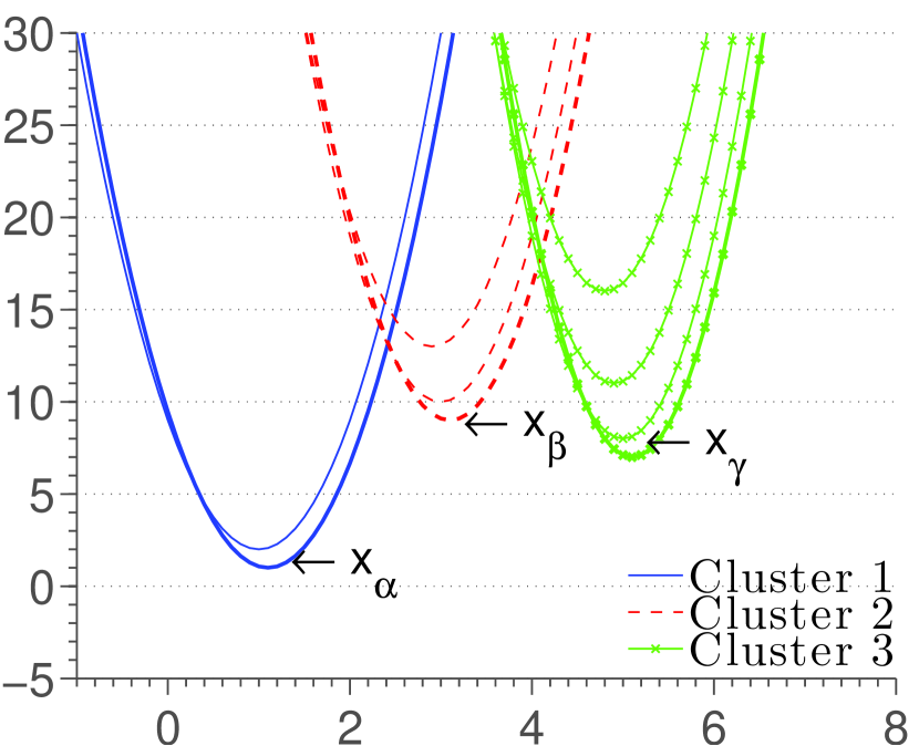
Figure 2: The case when only 3 quadratics are to be retained: three clusters are formed and within each, the quadratic with the lowest value is selected.

IV Illustrative Example

In this section we demonstrate the ideas described thus far on a two dimensional system with linear dynamics and a nonlinear output. The continuous time representation is

$$\frac{d}{dt}\left[\begin{array}[]{c}x_{1}(t)\\ x_{2}(t)\end{array}\right] =\left[\begin{array}[]{cc}0&0\\ 1&0\end{array}\right]\left[\begin{array}[]{c}x_{1}(t)\\ x_{2}(t)\end{array}\right]+\left[\begin{array}[]{c}1\\ 0\end{array}\right]w(t),$$ (88)

$$y(t) =\frac{(x_{2}(t))^{3}}{40}+v(t),$$ (89)

where $w(\cdot)$ and $v(\cdot)$ are the process disturbance and measurement noise respectively. Taking a sample time $\Delta t$ of $0.1$s, the discretized dynamics is

$$\left[\begin{array}[]{c}x_{1}(k+1)\\ x_{2}(k+1)\end{array}\right] =\left[\begin{array}[]{cc}1&0\\ 0.1&1\end{array}\right]\left[\begin{array}[]{c}x_{1}(k)\\ x_{2}(k)\end{array}\right]$$ (96)

$$\quad+\left[\begin{array}[]{c}0.1\\ 0\end{array}\right]\Delta w(k),$$ (99)

where $\Delta w(k)$ is the approximation corresponding to $w(k)\Delta t$ over the sampling time. As specified in Sec. III the implementation of the deterministic filter proceeds along three steps. The general steps as modified and applied to this specific example are as follows to this example are as follows.
1. generation of the quadratic approximation: In this case, the output equation (89) is

$$C(x)=\frac{x^{3}}{40}+v(k).$$ (100)

The contrained nonlinear optimization described in Sec. III-A admits the following simplification in the current case. Consider any window $\Omega$ with subpartitions $\Omega_{k}$ (recall Sec. III-A). In order to design the optimal quadratic approximation over such a set $\Omega_{k}$, we note that this problem is essentially a one dimensional regression (albeit with nonlinear constraints). We create a vector $x_{s}$ of $N$ sample points such that ${x_{s}}_{i}\in\Omega_{k}$ for all $i\in\{1,2,\ldots N\}$. Now to fit the (continuous) output function (or its square), denoted by $g(\cdot)$, over $\Omega_{k}$ using a quadratic

$$f(x)=\left(\begin{array}[]{cc}{x}^{T}&1\end{array}\right){\left[\begin{array}[]{cc}a_{2}&a_{1}/2\\ a_{1}/2&a_{0}\end{array}\right]}\left(\begin{array}[]{c}{x}\\ 1\end{array}\right),$$ (106)

the optimization problem reduces to solving a least squares fitting problem to determine the optimal coefficient vector $z:=[a_{2},a_{1},a_{0}]^{T}$ such that

$$Az =\left[\begin{array}[]{c}g({x_{s}}_{1})\\ g({x_{s}}_{2})\\ \vdots\\ g({x_{s}}_{N})\end{array}\right],$$ (111)

$$\text{where}\qquad A :=\left[\begin{array}[]{ccc}({x_{s}}_{1})^{2}&({x_{s}}_{1})&1\\ ({x_{s}}_{2})^{2}&({x_{s}}_{2})&1\\ \vdots&\vdots&\vdots\\ ({x_{s}}_{N})^{2}&({x_{s}}_{N})&1\end{array}\right].$$ (116)

The additional constraints are that $a_{2}\geq 0$ (for convexity) and that $f(x)\geq g(x),\,\,\forall x\in\Omega$. Solving this yields the desired quadratic bases. The min-plus basis obained by such a quadratic approximation over a window $\Omega$ centered around $x_{2}=2$ is as shown in Fig. 3.

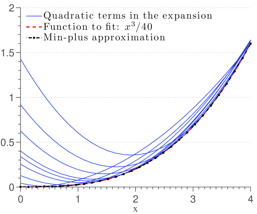
Figure 3: Min-plus expansion for the output function ${x_{2}}^{3}/40$ for a window centered around $x_{2}=2$.

2. The recursion to obtain the next set of quadratics (i.e. the min-plus basis expansion of the value function during the next time step) involves taking the sum of the various quadratic terms in (56). This is generated by taking the pairwise sum of the various quadratics available.

3. To reduce the dimensionality of the growth in basis terms we use a k-means based clustering approach [14] where the quadratics are clustered based on the locations of their argmin (ref. Sec. III-C). The simulation results of this filter design approach for the example considered are as shown in Fig. 4, 5. Note that although each window is only $2$ units in width, the use of the repeated window generation (a sliding window) leads to a filter capable of handling large measurement noises.

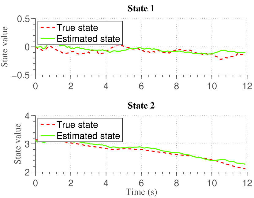
Figure 4: State filtering

Figure 5: Filtered measurement

V Conclusion and Future Directions

The details of the min-plus approach described herein generate filters for systems with nonlinear dynamics and nonlinear output. Its main novelty is in the utilization of the min-plus basis expansion of the value function coupled with the exploitation of the linearity of the dynamic programming operator over such a (semi)-field. The salient features of this approach as discussed herein, provide a structure which maybe used for a variety of applications. Further, the example serves as a template for future algorithmic developments. A few of the avenues along which a study of the different stages used in these methods may be pursued are: (1) generating optimal min-plus fitting techniques. The approach to fitting described herein provides one method (albeit not the optimal one); (2) the development of more sophisticated projection techniques for managing the growth in dimensionality (and an error analysis thereof); (3) the study of methods to speed up these stages. For instance some of the basis expansions may be done offline thereby helping speed up the real time operation of the implementation. The application of these methods to the real time estimation of signals in various domains is a potentially fruitful theme for future research.

References

- [1] W.H. Fleming, E. De Giorgi, Lefschetz Center for Dynamical Systems, Brown University. Center for Control Sciences, and Brown University. Division of Applied Mathematics. Deterministic nonlinear filtering. Annali della Scuola Normale Superiore di Pisa-Classe di Scienze-Serie IV, 25(3):435–454, 1997.
- [2] R. E. Mortensen. Maximum-likelihood recursive nonlinear filtering. Journal of Optimization Theory and Applications, 2:386–394, 1968. 10.1007/BF00925744.
- [3] A. Krener. The convergence of the minimum energy estimator. In Wei Kang, Carlos Borges, and Mingqing Xiao, editors, New Trends in Nonlinear Dynamics and Control and their Applications, volume 295 of Lecture Notes in Control and Information Sciences, pages 187–208. Springer Berlin / Heidelberg, 2003. 10.1007/978-3-540-45056-6_12.
- [4] J.C Willems. Deterministic least squares filtering. Journal of econometrics, 118(1):341–373, 2004.
- [5] R. Mahony, T. Hamel, and J.M. Pflimlin. Nonlinear complementary filters on the special orthogonal group. Automatic Control, IEEE Transactions on, 53(5):1203–1218, 2008.
- [6] E. Scholte and M. E. Campbell. A nonlinear set-membership filter for on-line applications. Int. J. Robust Nonlinear Control, 33:1337–1358, 2003.
- [7] V.P. Maslov. On a new principle of superposition for optimization problems. Russian Mathematical Surveys, 42:43, 1987.
- [8] W.H. Fleming and W.M. McEneaney. A Max-Plus-Based Algorithm for a Hamilton–Jacobi–Bellman Equation of Nonlinear Filtering. SIAM Journal on Control and Optimization, 38:683, 2000.
- [9] W.M. McEneaney. A curse-of-dimensionality-free numerical method for solution of certain HJB PDEs. SIAM Journal on Control and Optimization, 46(4):1239–1276, 2008.
- [10] S. Sridharan, Mile Gu, M.R. James, and W.M. Mc Eneaney. An efficient computational method for the optimal control of higher dimensional quantum systems. In Proceedings of the, 49th IEEE Conference on Decision and Control, pages 2996–3001, Atlanta, USA, December 15-17 2010.
- [11] W.M. McEneaney. Idempotent method for deception games and complexity attenuation⋆. In World Congress, volume 18, pages 4453–4458, 2011.
- [12] A.G. Kallapur, S. Sridharan, W.M. McEneaney, and I.R. Petersen. Min-plus techniques for set-valued state estimation. Arxiv preprint arXiv:1203.2846 (under review), 2012.
- [13] V.N. Kolokoltsov. Idempotent structures in optimization. Journal of Mathematical Sciences, 104(1):847–880, 2001.
- [14] D.J.C. MacKay. Information theory, inference, and learning algorithms. Cambridge Univ Pr, 2003.