Spin dynamics in a strongly driven system: very slow Rabi oscillations

Abstract

We consider joint effects of tunneling and spin-orbit coupling on driven by electric field spin dynamics in a double quantum dot with a multi-level resonance scenario. We demonstrate that tunneling plays the crucial role in the formation of the Rabi-like spin-flip transitions. In contrast to the linear behavior for weak electric fields, the spin flip rate becomes much smaller than expected for the two-level model and shows oscillating dependence on the driving field amplitude in stronger fields. In addition, the full spin flip is very difficult to achieve in a multi-level resonant system. These two effects have a similarity with the Zeno effect of slowing down the dynamics of an observable by its measurement. As a result, spin manipulation by electric field becomes much less efficient than expected.

I Introduction

Fast reliable spin manipulation in quantum dots is one of the challenges in spintronics and semiconductor-based quantum information. The design of corresponding gates can be based on electric dipole spin resonance where the spin-orbit coupling (SOC) Rashba1 ; Nowack ; Pioro ; Golovach06 allows on-chip spin manipulation by external electric field as well as electric read-out of spin states.Levitov03 Without external driving, SOC effects on localized in quantum dots electrons are very weak and lead to long spin relaxation times.Khaetskii01 ; Fabian05 The important questions here are how fast can the gate operate, what limits the manipulation rate, and how efficient is the spin manipulation in terms of the achievable spin configurations.GomezLeon11 It seems that a stronger driving field allows for a faster spin manipulation, as predicted in a simple Rabi picture of the driven oscillations. This picture is applicable for a single quantum dot with a parabolic confinement, where the electron displacement from the equilibrium is linear in the applied electric field.Jiang06 However, double quantum dots where tunneling plays the crucial role for the orbital dynamics, and the corresponding energy scales are different from a single quantum dot, are more promising for observation of new physics and applications in quantum information technologies.Petta05 The tunneling makes the description of the SOC puzzling since the electron momentum is not a well-defined quantity at under-the-barrier motion, and the tunneling rate can become strongly spin-dependent.Amasha ; Stano In addition, the double dots provide a possibility to study free and driven interacting qubits.Shitade11 ; Nowak Here we concentrate on one-dimensional systems attractive for spintronics Quay et al. (2010); Pershin, Nesteroff and Privman (2004); Malard11 and building quantum dots Nadj-Perge et al. (2010); Nadj-Perge2012 ; Bringer and Schäpers (2011) and consider spin manipulation in single-electron double quantum dot Ulloa06 ; Sanchez ; Wang ; Zhu ; Wang11 ; Borhani11 by periodic electric field.

We show that even for a basic quantum system such a single electron spin, the efficiency and time scale of the manipulation strongly depend on the electron orbital motion and, as result, to an unexpected dependence on the external electric field.diamond_science The nonlinearity of the spin and charge dynamics is expected to lead to unusual consequences on the driven spin behavior.Rashba11 In a multilevel system Rabi spin oscillations are slowed down if the field is sufficiently strong, which challenges efficient spin manipulation. We restrict ourselves to the single electron dynamics to demonstrate in the most direct way the nontrivial mutual effect of coordinate and spin motion on the Rabi oscillations. The slowing of the oscillations down at high electric fields is a truly unexpected general feature of a multi-level system compared to the conventional two-level model and thus can occur in a broad variety of structures.

This paper is organized as follows. In Section II we introduce quantum mechanical description of electron in a double quantum dot with spin-orbit coupling and magnetic field. Section III presents the model of driven dynamics. In Section IV we apply the stroboscopic Floquet approach for the long-time evolution and obtain the properties of Rabi oscillations under various conditions. Conclusions of this work are given in Section V.

II Model, Hamiltonian, and Observables

The unperturbed Hamiltonian $H_{0}={k^{2}}/{2m}+U(x)$ describes electron in a double quantum dot with the potential (see Fig.1) Khomitsky :

$$U(x)=U_{0}\left[-2\left(\frac{x}{d}\right)^{2}+\left(\frac{x}{d}\right)^{4}\right],$$ (1)

where $k=-i\partial/\partial x$ is the momentum operator and $\hbar\equiv 1$. The minima at $-d$ and $d$ are separated by a barrier of the height $U_{0}$. In the absence of external fields and SOC the ground state is split into the doublet of even ($\psi_{\rm g}$) and odd ($\psi_{\rm u}$) states. The tunneling energy $\Delta E_{g}\ll U_{0}$ determines the tunneling time $T_{\rm tun}=2\pi/\Delta E_{g}$. The Zeeman coupling to magnetic field $H_{Z}=\Delta_{Z}\sigma_{z}/2$, where $|\Delta_{Z}|$ is the Zeeman splitting.

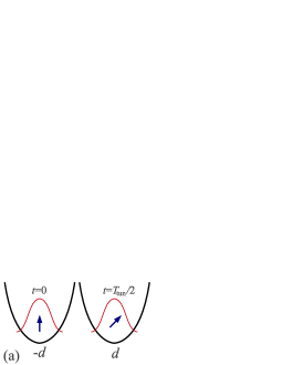
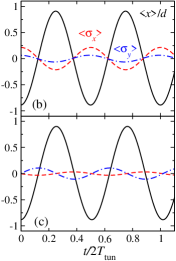
Figure 1: (Color online) (a) Qualitative picture of the spin dynamics induced by the interminima tunneling. (b,c) Free evolution of coordinate (solid line) and spin components $\langle\sigma_{x}\rangle$ (dashed line), $\langle\sigma_{y}\rangle$ (dashed-dot line) for $B=1.73$ T (b) and $B=6.93$ T (c). The initial state is the even combination of the states corresponding to the tunneling-split doublet with SOC taken into account.

The SOC has the form:

$$H_{\mathrm{so}}=\left(\alpha_{D}\sigma_{x}+\alpha_{R}\sigma_{y}\right)k,$$ (2)

where the bulk-originated Dresselhaus $\left(\alpha_{D}\right)$ and structure-related Rashba $\left(\alpha_{R}\right)$ parameters determine the strength of SOC. In the presence of SOC the spatial parity of the eigenstates is approximate rather than exact being the qualitative feature of the coupling linear in the odd $k$-operator, eventually resulting in the ability of spin manipulation by electric field.

The quantities we are interested in are the spin components:

$$\langle\sigma_{i}(t)\rangle=\int_{-\infty}^{\infty}\sigma_{i}(x,t)dx,$$ (3)

where $\sigma_{i}(x,t)={\bm{\psi}}^{\dagger}(x,t)\sigma_{i}{\bm{\psi}}(x,t)$ is the spin density, and expectation value of the coordinate

$$\langle x(t)\rangle=\int_{-\infty}^{\infty}x\rho(x,t)dx,$$ (4)

where $\rho(x,t)={\bm{\psi}}^{\dagger}(x,t){\bm{\psi}}(x,t)$, and ${\bm{\psi}}(x,t)$ is the two-component electron wavefunction.

For numerical studies we diagonalize exactly the time-independent Hamiltonian $H_{0}+H_{\mathrm{so}}+{H}_{Z}$ in the truncated spinor basis $\psi_{n}(x)|\sigma\rangle$, where $\psi_{n}(x)$ are the eigenfunctions of $H_{0}$ in Eq.(1), and $|\sigma\rangle$ where $\sigma=\pm 1$ corresponds to the spin parallel (antiparallel) to the $z$-axis, find corresponding eigenvalues, and obtain the new basis set $\left|\psi_{n}\right\rangle$. We consider below as an example a GaAs-based structure, where the effective mass is 0.067 of the free electron mass, with $d=25\sqrt{2}$ nm and $U_{0}=10$ meV. In the absence of magnetic field the ground state energy is $E_{1}=3.938$ meV, and the tunneling splitting $\Delta E_{g}=0.092$ meV, corresponding to the transition frequency close to 23 GHz. To illustrate the spin dynamics, we consider a moderate external magnetic field with $\Delta_{Z}=\Delta E_{g}/2$ corresponding to $B=1.73$ T, and a relatively strong magnetic field with $\Delta_{Z}=2\Delta E_{g}$ ($B=6.93$ T) with the Landé factor $g=-0.45$. The parameters of the SO coupling are assumed to be $\alpha_{R}=1.0\cdot 10^{-9}$ eVcm, and $\alpha_{D}=0.3\cdot 10^{-9}$ eVcm, however, our results can be applied to various double quantum dots with different SOC parameters and thus have a quite general character. In particular, the change in the interdot barrier shape and geometry would modify only quantitatively the system parameters, including the energy levels, spinor wavefunctions, and, as a result, the resonant driving frequency. The increase in the interdot distance would decrease the tunneling splitting, making such a system more sensitive to external influence from phonons, fluctuations in the driving field, etc.

III Driven dynamics

To demonstrate a nontrivial interplay of the tunneling and spin dynamics, we begin with the coordinate and spin evolution of the electron initially localized near the $-d$ minimum. Spin evolution of the state $\left(\left|\psi_{\rm g}\right>+\left|\psi_{\rm u}\right>\right)\left|1\right>/\sqrt{2}$ can be described approximately analytically taking into account four spin-split lowest levels and a simpler SOC Hamiltonian $\alpha_{R}\sigma_{y}k$ as

$$\langle\sigma_{x}(t)\rangle=\alpha_{R}\frac{K\Delta E_{g}}{A_{+}A_{-}}\sin(A_{+}t)\sin(A_{-}t)$$ (5)

where $K=-i\langle\psi_{\rm u}\left|k\right|\psi_{\rm g}\rangle$, which in the $\Delta E_{g}\ll U_{0}$ limit can be accurately approximated as $K=md\Delta E_{g}$, and $A_{\pm}=\sqrt{E_{\pm}^{2}/4+\alpha_{R}^{2}K^{2}}$, where $E_{\pm}=\Delta E_{g}\pm\Delta_{Z}$. Numerical results for coordinate and spin are shown in Fig.1. With the increase in magnetic field, the effect of SOC decreases, leading to smaller amplitudes of precession, as can be seen from comparison of Fig.1(b) and Fig.1(c). In addition, both the initial state and spin precession axis change leading to a different phase shift between the observed spin components.

Next we consider a periodic perturbation by electric field at $t>0$:

$$\mathcal{E}(t)=\mathcal{E}_{0}\sin(\widetilde{\omega}_{Z}t).$$ (6)

Here $\widetilde{\omega}_{Z}$ is the exact, taking into account SOC, frequency of the spin-flip transition. For the chosen set of parameters $\widetilde{\omega}_{Z}$ is very close to $\Delta_{Z}.$ The field strength is characterized by parameter $f$ defined as $e\mathcal{E}_{0}\equiv f\times U_{0}/2d$, where $e$ is the fundamental charge. For the chosen system parameters, $f=1$ corresponds to the electric field of approximately $1.5\times 10^{3}$ V/cm, similar to Ref.[Nowack, ]. Here we consider different regimes of the strength and see how the change in the shape of the quartic potential produced by the field becomes crucially important for the spin dynamics in two sets of energy levels produced by magnetic field. We build in the obtained $|\psi_{n}\rangle$ basis the matrix of the Hamiltonian $\widetilde{V}=ex\mathcal{E}_{0}\sin(\widetilde{\omega}_{Z}t)$ and study the full dynamics with the wavefunctions:

$${\bm{\psi}}(x,t)=\sum_{n}\xi_{n}(t)e^{-{i}E_{{n}}t}\left|\psi_{{n}}\right\rangle.$$ (7)

The time dependence of $\xi_{{n}}(t)$ is given by:

$$\frac{d\xi_{{n}}(t)}{dt}={i}e\mathcal{E}(t)\sum_{l}\xi_{l}(t)x_{{ln}}e^{-{i}\left(E_{{l}}-E_{{n}}\right)t},$$ (8)

where $x_{{ln}}\equiv\left\langle\psi_{{l}}\right|\widehat{x}\left|\psi_{{n}}\right\rangle$. There are two different types of $x_{ln}$: (1) matrix elements of the order of $d$ due to the different parity of the wavefunctions in the absence of SOC, and (2) those determined by the SOC strength. In the weak SOC limit $\left|\Delta_{Z}-\Delta E_{g}\right|\gg\alpha_{R}|K|$, the SO-determined matrix element of coordinate in the lowest spin-split doublet can be evaluated as

$$x_{\rm so}=2dK\alpha_{R}\frac{\Delta_{Z}}{\Delta_{Z}^{2}-\left(\Delta E_{g}\right)^{2}}.$$ (9)

In our calculations we assume that the initial state is the ground state of the full Hamiltonian, that is $\xi_{1}(0)=1$ and $\xi_{n>1}(0)=0$. The entire driven motion of the system can be approximately characterized as a superposition of two types of transitions: resonant “spin-flip” transitions with the matrix element of coordinate determined by the SOC and off-resonant “spin-conserving” transitions with a larger matrix element of coordinate.leakage Both types are crucially important for the understanding of the spin dynamics. With the estimate $K\approx m\Delta E_{g}d$, in both cases considered by us ($\Delta_{Z}=E_{g}/2$ and $\Delta_{Z}=2E_{g}$), we obtain $d\approx 10x_{\rm so}$. As a result, the off-resonant transitions are not weak compared to the required once. Throughout the calculation we neglect orbital and spin relaxation processes assuming that the driving force is sufficiently strong to prevent the decoherence on the time scale of the spin spin-flip transition. It is known that the periodic field forms a well-established driven dynamics even in the presence of damping as long as the level structure is not deeply disturbed by the broadening. For our parameters it means that one can expect the observation of the predicted results in the currently available semiconductor structures at temperatures moderately below 1 K.Nadj-Perge et al. (2010)

We begin with presentation of the short-time dynamics of coordinate $\langle x\rangle/d$ and spin $\langle\sigma_{x}\rangle$ for four initial periods of the driving field (Fig.2). These resuts were obtained by the explicit numerical integration of Eq.(8) with a time step on the order of $10^{-4}T_{Z}$. The other component $\langle\sigma_{z}\rangle$ changes much slower and will be treated later on a long timescale, which is the primary topic of our interest. It can be seen in Fig.2 that the fast oscillations are accompanying mainly the local variations of observables, especially of the spin. Considerable changes such as Rabi oscillations of spin can be achieved only after many periods of the driving field. We will focus on this slow dynamics below.

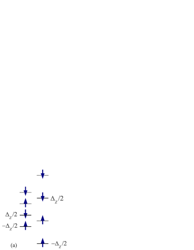
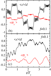
Figure 2: (Color online) (a) Scheme of the levels and spin components involved in the Zeeman resonance, $B=1.73$ T (left) and $B=6.93$ T (right), (b) short-term time-dependent $\langle x\rangle/d$ and $\langle\sigma_{x}\rangle$, as marked near the plots, induced by external field with $f=0.1$, $B$=1.73 T, $T_{Z}$=88 ps; (c) same as in (b) for $B$=6.93 T, $T_{Z}$=22 ps.

IV Floquet stroboscopic approach

To consider the long-term time dependence of the periodically driven system we apply the Floquet approach Shirley ; Platero ; Kohler05 ; Jiang06 ; Wu in the stroboscopic form. Here we remind the reader main features of this approach developed in Ref.[Demikhovskii, ]. As the first step, the one-period propagator matrix $\mathbf{U}_{ln}(T_{Z})$ is obtained by a high-precision numerical integration of the system (8) at one period of the driving $T_{Z}=2\pi/\widetilde{\omega}_{Z}$ in the basis of all unperturbed states. For numerically accurate $\mathbf{U}_{ln}(T_{Z})$, we obtain its eigenvalues $E_{Q}$ which are the quasienergies of the driven system, and the corresponding orthogonal eigenvectors $A^{Q}_{l}$. As a result, the one-period propagator $\mathbf{U}_{ln}(T_{Z})$ can be presented as:

$$\mathbf{U}_{ln}(T_{Z})=\sum_{Q}A^{Q}_{l}\left(A^{Q}_{n}\right)^{*}e^{-iE_{Q}T_{Z}}.$$ (10)

Its $N$-th power obtained by taking into account the orthogonality of the eigenvectors $A^{Q}_{l}$ gives the stroboscopic propagator $\mathbf{U}_{ln}(NT_{Z})$ for $N$ periods as

$$\mathbf{U}_{ln}(NT_{Z})=\sum_{Q}A^{Q}_{l}\left(A^{Q}_{n}\right)^{*}e^{-iE_{Q}NT_{Z}}.$$ (11)

For any integer $N$ the system state is given by $\left|\Psi(NT_{Z})\right\rangle=\mathbf{U}_{ln}(NT_{Z})\left|\Psi(0)\right\rangle$. The similarity of Eq.(10) for a single-period propagator and Eq.(11) for any $N\geq 1$ is a highly nontrivial fact demonstrating that ${U}_{ln}(NT_{Z})={U}_{ln}^{N}(T_{Z})$ can be simply expressed by the right-hand-side in Eq.(11). The stroboscopic approach allows us to study very accurately the long-time evolution since the $N$-period propagator (11) is constructed explicitly in a finite algebraic form. Although this propagator describes the dynamics exactly, it allows to watch only the stroboscopic evolution rather than the entire continuous one. However, if we are interested in slowly evolving phenomena such as chaos development Demikhovskii and Rabi oscillations which occur here on many periods of the driving field, the stroboscopic approach is fully justified and highly efficient. The experiment Nowack uses stroboscopic approach with the intervals on the order of 100 ns to measure the slow dynamics of the driven electron spin.

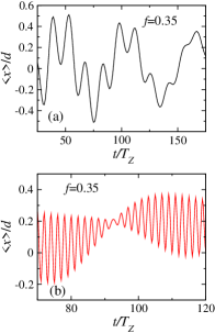
Figure 3: (Color online) Stroboscopic time dependence of $\langle x\rangle/d$ for field $f=0.35$ in a given time window: (a) $B=1.73$ T, (b) $B=6.93$ T. Solid lines serve only as a guide for the eye.

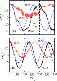
Figure 4: (Color online) Stroboscopic time dependence of $\langle\sigma_{z}(NT_{Z})\rangle$ for different external driving fields $f$ marked near the plots for two different magnetic fields: (a) $B=1.73$ T, vertical dashed line marks the operational definition of the spin-flip period, (b) same as in (a) for $B=6.93$ T.

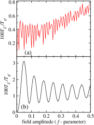
Figure 5: (Color online) Nonlinear dependence of the Rabi spin-flip frequency on the electric field amplitude in multilevel system for two different magnetic fields (a) $B=1.73$ T, the characteristic spin-flip rate of the order of 50 MHz, (b) $B=6.93$ T, the characteristic spin-flip rate of the order of 400 MHz.

The results of calculations of electron displacement at discrete times $NT_{Z}$ are presented in Fig.3. As one can see in Fig.3, the time dependence of the displacement becomes strongly nonperiodic with the typical values being considerably less than $d$. That is in a strong electric field the electron probability density redistribution between the dots is not complete. The motion can be qualitatively analyzed in the pseudospin model of the charge dynamics,Rashba11 where the tunneling splitting is described by the $\sigma_{z}$ matrix, and the driving field is coupled to the $\sigma_{x}-$matrix. The decrease in the electron displacement with the increase in the electric field can be viewed as a suppressed spin precession in a strong periodic field or as a coherent destruction of tunneling.Platero This nonperiodic behavior and decrease in the displacement eventually result in a less efficient spin driving. It should be mentioned that the fast oscillations in Fig.2 which are in general absent in Fig.3 reflect the difference between the continuous time scale in the former Figure and the stroboscopic Floquet times $NT_{Z}$ in the latter one. Figure 3 clearly illustrates the role of the spin in the orbital dynamics: the curves in Fig.3(a) and 3(b) are very different. Tracking of the system at stroboscopic times $NT_{Z}$ may not allow seeing the complete fast orbital dynamics, thus masking some details. As a result, there is no simple way to describe this stroboscopic picture directly in terms of the Hamiltonian parameters.

The slow long-term spin dynamics is presented in Fig.4. Here the ”unit of time” $T_{Z}$ is short enough and the time dependence of $\langle\sigma_{z}\rangle$ is accurately described by the stroboscopic approach. Since the spin dynamics is not strictly periodical and full spin flips do not always appear in this system, we use the operational definition of the “spin-flip” time $T_{sf}$: spin flip occurs when spin component shows a broad minimum albeit accompanied by fast oscillations (see in Fig.4(a)). The fast dynamics in the spin-flip doublet shown in Fig.4 becomes slow with the field increase as a result of a weaker effective coupling of the states with different parity. The resulting spin behavior, arising solely due to the SOC, is shown in Fig.4. The Rabi frequency for the spin-flip is smaller for some higher values of $f$ (which we vary through Fig.3-Fig.4) than for some weaker values of $f$ in contrast to what can be expected for the weak fields employed, e.g. in the experiments Nowack , being a manifestation of the generally nonmonotonous behavior of the Rabi frequency on the electric field amplitude. In addition, in contrast to the simple Rabi oscillations, the flips become incomplete, with $\left<\sigma_{z}(t)\right>=-1$ never reached. These two qualitative effects are the results of the enhanced electron tunneling between the potential minima: the spin precession in the driven interminima motion establishes corresponding spin dynamics and prevents the electric field to flip the spin efficiently. This effect makes a qualitative difference to the model of Ref.Nowack , where electron is assumed to be always located in the orbital ground state near the minimum of the potential formed by the parabolic confinement and weak external electric field.

To present a broader outlook onto the dependence of the spin flip rate on the driving field, we plot in Fig.5 the spin flip rate for $B=1.73$ T and $B=6.93$ T. In contrast to the linear dependence for a conventional two-level Rabi resonance formula, one can see a strongly different much more complicated non-monotonous dependence in a multi-level structure, especially at high fields. The regime in Fig.5(a) shows more irregularities since all four lowest levels are equidistant (Fig.2(a)) and involved in the resonance while in Fig.5(b) more regular dependence is observed, reflecting a simpler nature of the resonances here.

We would like to mention here that the observed slowing down of spin dynamics can be seen on a more general ground, not restricted to the exact form of Eq.(8), as the Zeno effect of freezing evolution of a measured quantity.Streed ; Echanobe ; Sokolovski10 Indeed, the operator $-i\sigma_{i}\partial/\partial x$ makes the orbital dynamics spin-dependent, and, as a result, performs the measurement of the $\sigma_{i}$ component Sokolovski11 ; Allahverdyan in the sense of von Neumann procedure. This can be seen in the evolution of a two-component wave function:Sokolovski11

$$e^{-\alpha t\sigma_{z}{\partial}/{\partial x}}\phi(x)\left(\zeta_{1}\left|1\right>+\zeta_{-1}\left|-1\right>\right)=$$

$$\phi(x-\alpha t)\zeta_{1}\left|1\right>+\phi(x+\alpha t)\zeta_{-1}\left|-1\right>,$$ (12)

where we took $i=z$ as an example, $\zeta_{1}$ and $\zeta_{-1}$ correspond to $\pm 1$ eigenvalues of $\sigma_{z}$, respectively, and $\alpha$ is the coupling constant. The SOC thus The SOC thus entangles the orbital and spin motion, destroys the coherent superposition of spin-up and spin-down states, and performs the von Neumann-like spin measurement by mapping spin state on the electron position. This von Neumann measurement, is, however, different from the experimental measurement procedure applied, e.g. in Ref.[Nowack, ]. The spin-orbit coupling coupling drives the coherent superposition of different spin components and at the same time, by constant strong measurement, destroys it leading to a slow spin dynamics.

V Conclusions

We have considered the interplay between the tunneling and spin-orbit coupling in a driven by an external electric field one-dimensional single-electron double quantum dot. In the regime of the electric dipole spin resonance, where the electric field frequency exactly matches the Zeeman transition, the complex interplay of these mechanisms results in two unexpected effects. The first effect is the nonmonotonous change in the Rabi spin oscillations frequency with the electric field amplitude. The Rabi oscillations become much slower than expected for a two-level system. The second effect is the incomplete Rabi spin flips. This behavior results from the fact that the interminima motion establishes a competing spin dynamics, leading to the physics somewhat similar to the Zeno effect, preventing a fast change in a measured quantity. These results indicating the slowdown and nonlinearity of the spin resonance in multilevel systems can be useful for pointing out certain fundamental challenges for the future experimental and spintronics device applications of phenomena based on spins in double quantum dots.

VI Acknowledgements

D.V.K. is supported by the RNP Program of Ministry of Education and Science RF, and by the RFBR (Grants No. 11-02-00960a, 11-02-97039/Regional). This work of EYS was supported by the MCINN of Spain Grant FIS2009-12773-C02-01, by ”Grupos Consolidados UPV/EHU del Gobierno Vasco” Grant IT-472-10, and by the UPV/EHU under program UFI 11/55.

References

- (1) E. I. Rashba and Al. L. Efros, Phys. Rev. Lett. 91, 126405 (2003).
- (2) K.C. Nowack, F.H.L. Koppens, Yu.V. Nazarov, and L.M.K. Vandersypen, Science 318, 1430 (2007).
- (3) M. Pioro-Ladriere, T. Obata, Y. Tokura, Y.-S. Shin, T.Kubo, K. Yoshida, T. Taniyama, and S. Tarucha, Nature Physics 4, 776 (2008).
- (4) V.N. Golovach, M. Borhani, and D. Loss, Phys. Rev. B 74, 165319 (2006).
- (5) L.S. Levitov and E.I. Rashba, Phys. Rev. B 67, 115324 (2003).
- (6) A.V. Khaetskii and Yu.V. Nazarov, Phys. Rev. B 64, 125316 (2001).
- (7) P. Stano and J. Fabian, Phys. Rev. Lett. 96, 186602 (2006).
- (8) Driving by ac magnetic fields was analyzed in detail in: A. Gómez-León and G. Platero, Phys. Rev. B 84, 121310(R) (2011).
- (9) J.H. Jiang, M.Q. Weng, and M.W. Wu, J. Appl. Phys. 100, 063709 (2006).
- (10) J. R. Petta, A. C. Johnson, J. M. Taylor, E. A. Laird, A. Yacoby, M. D. Lukin, C. M. Marcus, M. P. Hanson, and A. C. Gossard, Science 309, 2180 (2005).
- (11) S. Amasha, K. MacLean, I. P. Radu, D. M. Zumbühl, M. A. Kastner, M. P. Hanson, and A. C. Gossard, Phys. Rev. B 78, 041306 (2008).
- (12) P. Stano and P. Jacquod, Phys. Rev. B 82, 125309 (2010).
- (13) A. Shitade, M. Ezawa, and N. Nagaosa, Phys. Rev. B 82, 195305 (2010).
- (14) M. P. Nowak and B. Szafran, Phys. Rev. B 81, 235311 (2010); M. P. Nowak and B. Szafran, Phys. Rev. B 82, 165316 (2010).
- Quay et al. (2010) C. H. L. Quay, T. L. Hughes, J. A. Sulpizio, L. N. Pfeiffer, K. W. Baldwin, K. W. West, D. Goldhaber-Gordon, and R. de Picciotto, Nat. Phys 6, 336 (2010).
- Pershin, Nesteroff and Privman (2004) Y. V. Pershin, J. A. Nesteroff, and V. Privman, Phys. Rev. B 69, 121306 (2004).
- (17) M. Malard, I. Grusha, G. I. Japaridze, and H. Johannesson, Phys. Rev. B 84, 075466 (2011).
- Nadj-Perge et al. (2010) S. Nadj-Perge, S. Frolov, E. Bakkers, and L. Kouwenhoven, Nature 468, 1084 (2010).
- (19) S. Nadj-Perge, V.S. Pribiag, J.W.G. van den Berg, K. Zuo, S.R. Plissard, E.P.A.M. Bakkers, S.M. Frolov, and L.P. Kouwenhoven, arXiv:1201.3707 (2012).
- Bringer and Schäpers (2011) A. Bringer and T. Schäpers, Phys. Rev. B 83, 115305 (2011).
- (21) C.L. Romano, P.I. Tamborenea, and S.E. Ulloa, Phys. Rev. B 74, 155433 (2006); C.L. Romano, S.E. Ulloa, and P.I. Tamborenea, Phys. Rev. B 71, 035336 (2005).
- (22) R. Sánchez, E. Cota, R. Aguado, and G. Platero, Phys. Rev. B 74, 035326 (2006); E. Cota, R. Aguado, C.E. Creffield and G. Platero, Nanotechnology 14, 152 (2003).
- (23) M. Borhani and X. Hu, arXiv:1110.2193.
- (24) M. Wang, Y. Yin, and M. W. Wu, J. Appl. Phys. 109, 103713 (2011).
- (25) Z.-G. Zhu, C.-L. Jia, and J. Berakdar, Phys. Rev. B 82, 235304 (2010); J. Wätzel, A. S. Moskalenko, and J. Berakdar, Appl. Phys. Lett. 99, 192101 (2011).
- (26) L. Wang and M. W. Wu, J. Appl. Phys. 110, 043716 (2011).
- (27) A very interesting example of such a dependence was recently presented for a different promising for quantum information system such as nitrogen vacancy in diamond: G. D. Fuchs, V. V. Dobrovitski, D. M. Toyli, F. J. Heremans, and D. D. Awschalom, Science 326, 1520 (2009).
- (28) E.I. Rashba, Phys. Rev. B 84, 241305 (2011).
- (29) D. V. Khomitsky and E. Ya. Sherman, Phys. Rev. B 79, 245321 (2009).
- (30) These transitions, where the probability leaks to undesired off-resonance states, are unavoidable in superconducting solid-state realizations of qubits, too: E. Lucero, M. Hofheinz, M. Ansmann, R. C. Bialczak, N. Katz, M.Neeley, A. D. O Connell, H. Wang, A. N. Cleland, and J.M. Martinis, Phys. Rev. Lett. 100, 247001 (2008), J. M. Chow, J. M. Gambetta, L. Tornberg, J. Koch, L.S. Bishop, A. A. Houck, B. R. Johnson, L. Frunzio, S. M. Girvin, and R. J. Schoelkopf, Phys. Rev. Lett. 102, 090502 (2009); F. Motzoi, J. M. Gambetta, P. Rebentrost, and F. K. Wilhelm, Phys. Rev. Lett. 103, 110501 (2009).
- (31) J. H. Shirley, Phys. Rev. 138, B979 (1965).
- (32) G. Platero and R. Aguado, Physics Reports 395, 1 (2004).
- (33) S. Kohler, J. Lehmann, and P. Hänggi, Physics Reports 406, 379 (2005).
- (34) J. H. Jiang and M. W. Wu, Phys. Rev. B 75, 035307 (2007).
- (35) V. Ya. Demikhovskii, F. M. Izrailev, and A. I. Malyshev, Phys. Rev. E 66, 036211 (2002); V. Ya. Demikhovskii, F. M. Izrailev, and A. I. Malyshev, Phys. Rev. Lett. 88, 154101 (2002).
- (36) E. W. Streed, J. Mun, M. Boyd, G. K. Campbell, P. Medley, W. Ketterle, and D. E. Pritchard, Phys. Rev. Lett. 97, 260402 (2006).
- (37) J. Echanobe, A. del Campo, and J. G. Muga, Phys. Rev. A 77, 032112 (2008).
- (38) D. Sokolovski, Phys. Rev. A 84, 062117 (2011).
- (39) D. Sokolovski and E. Ya. Sherman, Phys. Rev. A 84, 030101 (2011).
- (40) Other approaches to spin measurement were recently introduced by A. E. Allahverdyan, R. Balian, and Th. M. Nieuwenhuizen, Phys. Rev. Lett. 92, 120402 (2004) and R. Ruskov, A. N. Korotkov, and K. Mølmer, Phys. Rev. Lett. 105, 100506 (2010).