Semiclassical Loop Quantum Gravity and Black Hole Thermodynamics

Semiclassical Loop Quantum Gravity
and Black Hole Thermodynamics

Arundhati DASGUPTA

A. Dasgupta

University of Lethbridge, 4401 University Drive, Lethbridge T1K 7R8, Canada arundhati.dasgupta@uleth.ca

Received March 22, 2012, in final form February 05, 2013; Published online February 16, 2013

In this article we explore the origin of black hole thermodynamics using semiclassical states in loop quantum gravity. We re-examine the case of entropy using a density matrix for a coherent state and describe correlations across the horizon due to ${\rm SU}(2)$ intertwiners. We further show that Hawking radiation is a consequence of a non-Hermitian term in the evolution operator, which is necessary for entropy production or depletion at the horizon. This non-unitary evolution is also rooted in formulations of irreversible physics.

black holes; loop quantum gravity; coherent states; entanglement entropy

83C57; 81Q35; 81T20

1 Introduction

With new results in lattice gravity, loop quantum gravity (LQG) and various other approaches to quantum gravity, there is hope that we might find the quantum of space-time [2, 39, 4, 41, 22, 21]. Though unifying gravity with other forces of nature will remain a puzzle. General theory of relativity is a theory of gravity and quantum field theory is the theory of particle dynamics and both are experimentally verified. Yet when we describe quantum fields in gravitational backgrounds, new phenomena arise which seem to signify the existence of new physics. Black hole thermodynamics and Hawking radiation are particularly interesting phenomena. The laws of black hole mechanics derived in [7] were the first indication that the black hole might be a system similar to a thermodynamic ensemble. The area increasing theorem [26] led to the conjecture that the entropy of the thermodynamic system is proportional to the area of the horizon [9]. The area of the horizon divided by four Planck length squared today is known as the Bekenstein–Hawking entropy. The use of quantum fields near the horizon then showed that black holes emit radiation in thermal spectrum at a temperature given by the surface gravity of the black hole [27], and the Planck’s constant naturally got included in the quantification of entropy, temperature etc. This confirmed that there is a ‘quantisation’ of the space-time and the microscopic structure will explain the origin of thermodynamic quantities. There are several explanations of the nature of the microscopic structure of the black hole entropy [39, 4], and the origin of thermodynamics, some of which will be reported in this volume. In this article I shall discuss the use of ‘coherent states’ in LQG to derive the physics of the system [25, 42]. The use of coherent states is well known in quantum electrodynamics in particular for lasers, and we will use similar coherent states for gravity. Once the coherent states are identified for the black hole, the derivation of thermodynamics follows the standard entropy formulation of correlated systems, part of which has been traced away [18]. A reduced density matrix is derived for a region outside the horizon and the wavefunction inside the horizon is traced over. This reduced density matrix gives an entropy proportional to the area of the horizon. There are semiclassical corrections to the Bekenstein–Hawking term, and the nature of the corrections is a function of the discretisation or graph embeddings used to describe the system [19]. In this article we describe the derivation of entropy using coherent states, and discuss briefly the nature of correlations which arise due to the gauge invariant coherent states using ${\rm SU}(2)$ intertwiners. These calculations are a preliminary indication of what a ‘physical coherent state’ might carry as correlations at the horizon [15]. The correlations make the state inside the horizon ‘entangled’ with the state outside the horizon.

As the coherent state is defined in the canonical formalism where space-time is foliated with constant time slices, the coherent state in discussion is defined in one time slice, which we take as the initial time slice. We then use a semi-classical Hamiltonian to evolve the coherent state in time. The derivation of time evolution is trivial if we restrict the evolution operator to be unitary. Non-trivial evolution occurs if the classically forbidden regions behind the horizon get exposed using a non-Hermitian term added to the Hamiltonian which facilitates entropy production [17, 20]. The change in entropy of the black hole is carried away as Hawking flux which escapes to infinity. This time evolution is irreversible in nature and is very similar to such time evolutions in complex systems [34].

In the next section we briefly describe coherent states for gravity. We also review the concept of entanglement entropy in this section. The third section describes the origin of entropy using a density matrix. It includes a description of the tracing mechanism when the coherent state is defined using intertwiners at vertices. In the fourth section we describe time evolution and the relation of this entropy production process to physics of complex systems. The fifth section discusses the results and the open problems yet to be solved using this formalism.

2 Coherent states in loop quantum gravity

The coherent states are useful semiclassical states in a quantum theory. In case of the simple harmonic oscillator or in quantum electrodynamics, these can be formulated as the eigenstate of the annihilation operator. Explicitly

$$\hat{a}|\psi\rangle=z|\psi\rangle,$$

where $\hat{a}$ is the annihilation operator for the positive energy modes of the theory and $z$ is the eigenvalue. These are usually Gaussians, e.g. for the harmonic oscillator

$$\psi=\frac{1}{\sqrt{2\pi\hbar}}\exp\left(-\frac{(x-z)^{2}}{2\hbar}\right),$$

where $z=x_{0}+ip_{0}$ is a point in the classical complexified phase space, $\hbar=h/2\pi$, and $h$ is Planck’s constant. Thus the coherent state is a Gaussian ‘peaked’ on the classical phase space point. In these coherent states the expectation values of operators are obtained as their classical values and trajectories also evolve along classical paths, preserving the coherence.

The coherent states appear as the kernel of a transformation from the Hilbert space $L^{2}({\mathbb{R}})$ to the Segal–Bergmann representation of the wave functions or $H({\mathbb{C}})\cap L^{2}({\mathbb{C}})$ [25]. Using the definition of the coherent state as a kernel Hall [25] generalised the coherent states to obtain those defined for a ${\rm SU}(2)$ Hilbert space. These appear as kernels in the transformation from the ${\rm SU}(2)$ Hilbert space to the intersection of the Hibert space defined in the complexified ${\rm SU}(2)$ phase space which incidentally is ${\rm SL}(2,{\mathbb{C}})$ space. These are therefore often named as ‘complexifier coherent states’. In a particular definition of the kernel, it is obtained as

$$K(h,g)=e^{\frac{t}{2}\Delta}\delta(h^{\prime},h)_{h^{\prime}\rightarrow g},$$ (2.1)

where $h$ is a ${\rm SU}(2)$ element, and $g$ is a ${\rm SL}(2,{\mathbb{C}})$ element, $\Delta$ is the Laplacian on the group manifold, $t$ is a parameter. The Hall coherent states can be directly applied to gravity as written in terms of LQG variables gravity is a ${\rm SU}(2)$ theory [42].

We begin by writing gravity in terms of LQG variables. The phase space of loop quantum gravity is obtained using a canonical formulation of gravity. The manifold is taken diffeomorphic to $\Sigma\times{\mathbb{R}}$. The $\Sigma$ slices foliate the space-time, and using the ADM metric, the dynamical variables are identified as the intrinsic metric $q_{ab}$ of the slice and the extrinsic curvature $K_{ab}$ with which the slices are embedded in the space-time. The intrinsic metric can be written in terms of the tangent space triads or soldering forms $e^{I}_{a}$. The phase space for LQG is again a redefinition of these and described thus [41, 22, 21]

$$A_{a}^{I}=\Gamma_{a}^{I}-\beta K_{ab}e^{Ib},\qquad E^{a}_{I}=\frac{1}{\beta}(\det e)e^{a}_{I},$$ (2.2)

where $e_{a}^{I}$ are the usual triads the ‘square root’ of the metric $q_{ab}=e_{a}^{I}e_{b}^{I}$, $K_{ab}$ is the extrinsic curvature, $\Gamma_{a}^{I}$ are the associated spin connections to the triads, $\beta$ is the one parameter ambiguity, which is known as the Immirzi parameter. The quantisation of the Poisson algebra of these variables is done by smearing the connection along one dimensional edges $e$ of length $\delta_{e}$ of a graph $\Gamma$ to get holonomies $h_{e}(A)$. The triads are smeared in a set of 2-surface decomposition of the three dimensional spatial slice to get the corresponding momentum $P_{e}^{I}$. (The momenta are also labeled by the edges as each edge intersects the corresponding 2 surface once by construction, or every edge has a corresponding unique two surface and vice versa.) The regularised LQG variables are

$$h_{e}(A)={\cal P}\exp\left(\int_{e}A\right),\qquad P_{e}^{I}=\int_{S}*E^{I}.$$ (2.3)

The algebra is then represented in a kinematic ‘Hilbert space’, in which the physical constraints have been ‘formally’ realised. Once the phase space variables have been identified, one can write a coherent state for these [25], i.e. minimum uncertainty states peaked at classical values of $h_{e}$, $P^{I}_{e}$ for one edge of the graph. The tensor product of these coherent states for each edge of the graph gives the coherent state for the entire space-time. Using the Peter–Weyl theorem for the delta function $\delta(h,h^{\prime})=\sum_{j}(2j+1)\chi_{j}\big{(}h^{\prime}h^{-1}\big{)}$, where $\chi_{j}$ is the character of the $j$th representation of ${\rm SU}(2)$, the complexifier coherent state (2.1) can be written as

$$\tilde{\psi}^{t}(g_{e})=\sum_{j}(2j+1)e^{-tj(j+1)/2}\chi_{j}\big{(}g_{e}h_{e}^{-1}\big{)}.$$ (2.4)

These are coherent states peaked at the classical holonomy with a width controlled by the parameter $t$. A ‘momentum representation’ of this is obtained by defining a Fourier transform which is such that the ‘momentum eigenstate’ $|jmn\rangle$ gives

$$\langle h|jmn\rangle=\pi_{j}(h)_{mn},\qquad\hat{P}_{e}|jmn\rangle=j(j+1)\hbar|jmn\rangle.$$

The $|jmn\rangle$ are thus the usual basis spin network states given by $\sqrt{2j+1}\pi_{j}(h_{e})_{mn}$ (normalised in the $h_{e}$ basis), which is the $mn$ element of the $j$th irreducible representation of the ${\rm SU}(2)$ matrix $h_{e}$, and $\hat{P}_{e}=\sqrt{\hat{P}_{e}^{I}\hat{P}_{e}^{I}}$. Taking the scalar product of the configuration coherent state (2.4) with the momentum eigenstate gives the momentum ‘coherent state’ as $\psi^{t}_{e}=e^{-tj(j+1)/2}\pi_{j}(g_{e})_{jmn}$, where $\pi_{j}(g_{e})_{mn}$ is the $j$th irreducible representation of the ${\rm SL}(2,{\mathbb{C}})$ element $g_{e}$. Thus the coherent state in the momentum representation is

$$|\psi^{t}(g_{e})\rangle=\sum_{jmn}e^{-tj(j+1)/2}\pi_{j}(g_{e})_{mn}|jmn\rangle.$$

In the above $g_{e}$ is a complexified classical phase space element $e^{iT^{I}P^{I\rm cl}_{e}/2}h^{\rm cl}_{e}$, where $P^{I\rm cl}_{e}$ and $h^{\rm cl}_{e}$ represent classical momenta and holonomy obtained by embedding the edge in the classical metric and $T^{I}$ are ${\rm SU}(2)$ generators. The $j$ is the quantum number of the ${\rm SU}(2)$ Casimir operator in that representation, and $m$, $n$ represent azimuthal quantum numbers which run from $-j,\dots,j$. Similarly, $(2j+1)\times(2j+1)$-dimensional representations of the $2\times 2$ matrix $g_{e}$ are denoted as $\pi_{j}(g_{e})_{mn}$. The coherent state is precisely peaked with maximum probability at the $h^{\rm cl}_{e}$ for the variable $h_{e}$ as well as the classical momentum $P_{e}^{I\rm cl}$ for the variable $P_{e}^{I}$. The fluctuations about the classical value are controlled by the parameter $t$ (the semiclassicality parameter). This parameter is given by $l_{p}^{2}/a$ where $l_{p}$ is Planck’s constant and $a$ is a dimensional constant which characterises the system. For the Schzwarzschild black hole $a$ can be taken as proportional to the area of the horizon. The coherent state for an entire slice can be obtained by taking the tensor product of the coherent state for each edge which form a graph $\Gamma$,

$$\Psi_{\Gamma}=\prod_{e}\psi^{t}_{e}.$$ (2.5)

Thus we are considering a semiclassical state, which is a state such that expectation values of operators are closest to their classical values. The information of the classical phase space variables are encoded in the complexified ${\rm SU}(2)$ elements labeled as $g_{e}$. The fluctuations over the classical values are controlled by the semiclassical parameter $t$.

The density matrix which describes the entire black hole slice is obtained as

$$\rho^{\rm total}=|\Psi_{\Gamma}\rangle\langle\Psi_{\Gamma}|,$$

where $|\Psi_{\Gamma}\rangle$ is the coherent state wavefunction for the entire slice, a tensor product of coherent state for each edge. These coherent states have been studied in various other forms [23, 10]. In this paper we also discuss the ${\rm SU}(2)$ invariant coherent state described in [42] using intertwiners at the vertices. We will describe the detailed derivation of the intertwiners for a particular graph in the next section using this generalisation. We should mention that previously other semiclassical states had been considered in the framework LQG known as weave states [5], but none have been yet used to describe black hole entropy. Coherent states have been used to describe quantum cosmology and FLRW universes [32]. Relatively recent reviews on approaches to black hole entropy and corrections to black hole entropy in LQG can be found in [6, 33, 14]. A review of black hole entropy in LQG and recent description of two dimensional black hole evaporation can be found in [3]. Before we begin the discussion on derivation of entropy using density matrices, we briefly describe the concept of ‘entanglement entropy’ and its use in quantum field theory in curved space-time to describe entropy of black holes. Our derivation will be totally ‘gravitational in origin’ defined using the LQG phase space variables.

3 Entanglement entropy

In quantum field theory, we use the definition of entropy due to von Neumann. It is defined thus given a density matrix $\rho$

$$S=-\operatorname{Tr}(\rho\ln\rho).$$

If the state is pure the entropy is zero, if the state is mixed the entropy is obtained as non-zero. This could be a system in which part of the wavefunction or the state of the system has been traced away. The tracing can be done for systems which have a product Hilbert spaces: e.g. $H=H_{I}\otimes H_{O}$. The $H_{I}$ is the Hilbert space which defines the ‘internal space’, $H_{O}$ is the outside Hilbert space. The basis states also thus appear in the product structure $|i\rangle\otimes|j\rangle$. The states are said to be entangled if the coefficients of the basis states do not factorise, e.g.

$$|\psi\rangle=\sum_{ij}d_{ij}|i\rangle|j\rangle$$

is entangled if

$$d_{ij}\neq d_{i}d_{j}.$$ (3.1)

A density matrix defined thus

$$\rho=|\psi\rangle\langle\psi|$$

can have a partial trace performed on it,

$$\operatorname{Tr}\rho=\sum d^{*}_{ij}d_{ji^{\prime}}|i\rangle\langle i^{\prime}|,$$

and the entropy computed using the above. We will now describe the ‘entanglement entropy’ of quantum fields in a black hole background. This shed light on why the entropy was proportional to the area of the horizon and not the volume of the black hole. A review on entanglement entropy of black holes can be found in [37]. Srednicki computed the entanglement entropy of a quantum field, where the field enclosed in a sphere of radius ‘$R$’ is traced out. The entropy of the remaining space-time is proportional to the area of the sphere [38]. This was a very interesting calculation however doing a similar calculation for a black hole background did not give finite answers. The reason is that the ‘metric’ in the coordinates of an outside observer is singular at the horizon. The near horizon volume is infinite, and thus the entropy due to the quantum fields in this volume is also infinite. ’t Hooft [40] introduced a mass dependent ‘cutoff’ as if a brickwall was steeling off the quantum fields, which satisfied a Dirichlet boundary condition at the wall. The presence of the brick wall could be used to obtain a finite value for the entropy. We shall briefly review the procedure here.

3.1 The brickwall model

The scalar field $\phi$ is taken in the background of a Schwarzschild black hole whose metric in spherical coordinates is

$$ds^{2}=-\left(1-\frac{2M}{r}\right)dt^{2}+\left(1-\frac{2M}{r}\right)^{-1}dr^{2}+r^{2}\big{(}d\theta^{2}+\sin^{2}\theta d\phi^{2}\big{)},$$ (3.2)

where $M$ is the mass of the black hole, $G=1$, $c=1$.

The scalar field’s Klein–Gordon equation in this background is

$$\frac{1}{\sqrt{-g}}\partial_{\mu}\left(\mathop{\sqrt{-g}}g^{\mu\nu}\partial_{\nu}\phi\right)-m^{2}=0.$$

Using the inverse of the metric (3.2) one finds that the Klein–Gordon equation is

$$\left(1-\frac{2M}{r}\right)^{-1}\left({-\partial_{t}^{2}}\right)\phi+\frac{1}{r^{2}}\partial_{r}\left(r^{2}\left(1-\frac{2M}{r}\right)\partial_{r}\right)\phi+\frac{1}{r^{2}}L^{2}\phi-m^{2}\phi=0,$$

where $L^{2}$ is the angular momentum operator. The above can be solved in the eikonal approximation using

$$\phi=e^{iEt}e^{i\int kdr},$$

where

$$k^{2}=\frac{r^{2}}{r(r-2M)}\left(\left(1-\frac{2M}{r}\right)^{-1}E^{2}-\frac{1}{r^{2}}l(l+1)-m^{2}\right).$$

As evident the wavenumber is quite big near the horizon, justifying the eikonal approximation (the phase dominates). Due to the Dirichlet boundary condition, $\phi=0$ at the wall, a particular value of the radius taken as $r=2M+h$ and an outer boundary $L$, the wavefunction’s wavenumber gets quantised as integer multiples of $\pi$

$$\pi n=\int_{2M+h}^{L}kdr.$$

The total number of such eigenmodes with energy $E$ is therefore the sum over angular momentum (each with $2l+1$) degeneracy

$$\int(2l+1)dl\pi n=g(E).$$

Given this one can compute

$$e^{-\beta F}=\prod_{n,l,l_{3}}\frac{1}{1-e^{-\tilde{\beta}E}},$$

where $F$ is the free energy, and the righthand side is the thermal distribution, at a temperature $1/\tilde{\beta}$, such that

$$\pi\tilde{\beta}F=\int dg(E)\log\big{(}1-e^{\tilde{\beta}E}\big{)}=-\int_{0}^{\infty}dE\frac{g(E)}{e^{\tilde{\beta}E}-1}.$$

Using the value of $g(E)$

$$F=-\frac{1}{\pi}\int_{0}^{\infty}~{}dE~{}\int_{2M+h}^{L}dr\left(1-\frac{2M}{r}\right)^{-1}\int\frac{(2l+1)}{\big{(}e^{\tilde{\beta}E}-1\big{)}}dl\sqrt{E^{2}-\left(1-\frac{2M}{r}\right)\left(\frac{l(l+1)}{r^{2}}\right)}$$

(we use the approximation that the scalar fields are massless). $F$ is then approximated in [40] as

$$F=-\frac{2\pi^{3}}{45h}\left(\frac{2M}{\tilde{\beta}}\right)^{4}-\frac{2}{9\pi}L^{3}\int_{0}^{\infty}\frac{dEE^{3}}{e^{\tilde{\beta}E}-1}.$$

Using the definition of entropy

$$S=\tilde{\beta}(U-F),\qquad U=\frac{\partial}{\partial\tilde{\beta}}\big{(}\tilde{\beta}F\big{)}$$

one obtains $S=4M^{2}$. This is indeed proportional to the area of the horizon, but one had to put the cutoff radius $h=\frac{1}{720\pi M}$, a very particular value to achieve the result.

There are some observations about this derivation of entropy: $(i)$ There is no entanglement of modes across the horizon of the QFT modes, what this represents is the entropy of a gas of scalar particles outside the horizon. $(ii)$ Even though the cutoff is mass dependent the proper-distance of the brickwall from the horizon is a constant. The question still remains why it is this constant and not another one.

3.2 Scalar entanglement for a bifurcate horizon

It is very interesting that this ‘entropy of a gas of scalar particles’ using the brick wall method could be placed in an ‘entanglement entropy’ context. In this formalism one traces over the ‘outside modes’ to obtain a density matrix and the entropy of the resultant partially traced sector of the system. The details of this derivation can be found in [8] and references therein. The crux of the computation is hinged on the definition of the wavefunction of the black hole as a ‘path-integral’ in a space-time with a complex metric. The space-time is the complexified Kruskal extension of the Schwarzschild black hole. The metric in spherical coordinates for the Schwarzschild black hole is given in (3.2). One then defines the Kruskal coordinates as

$$U=-e^{-(t-r-2M\ln(r/2M-1))/4M},\qquad V=e^{(t+r+2M\ln(r/2M-1))/4M},$$

$$UV=\left(1-\frac{r}{2M}\right)\exp\left(\frac{r}{2M}\right),$$

such that the Kruskal metric is

$$ds^{2}=\frac{-32M^{3}}{r}\exp^{-\left(r/2M\right)}dUdV+r^{2}d\Omega^{2}.$$

As evident the metric is extendible past $r=2M$, the horizon, and the horizon is bifurcate, with $V=0$ coinciding with the past horizon and $U=0$ coinciding with the future horizon. There are two asymptotics, and the transformations $U\rightarrow-U$ and $V\rightarrow-V$ map the two asymptotics. One could then define the Lorentzian metric as the real section of a complex metric, by defining the coordinates $U$ and $V$ w.r.t. a ‘complex time’ $z=\tau+it$. The $\tau$ is the Euclidean time, and it is such that in the Euclidean section $-2\pi M<\tau<+2\pi M$. The two asymptotics are then connected in some sense through this ‘Euclidean’ section. The complexified coordinates are

$$U=-e^{(iz-i2\pi M+r+2M\ln(r/2M-1))/4M},\qquad V=e^{(-iz+i2\pi M+r+2M\ln(r/2M-1))/4M}.$$

Clearly as the imaginary time $\tau$ changes from $-2\pi M$ to $2\pi M$, one travels from one asymptotics to another given by $z^{+}=2\pi M+it$ and $z^{-}=-2\pi M+it$ ($-\infty<t<\infty$) in complex time.

One defines a path-integral through the Euclidean throat which could be labeled as the propagator connecting the two asymptotics, with $\phi\equiv\phi_{+}$ in one and $\phi\equiv\phi_{-}$ in the other.

Define

$$\Psi(\phi_{-},\phi_{+})=\langle\phi_{-}|\exp(-\tilde{\beta}\hat{H}/2)|\phi_{+}\rangle.$$ (3.3)

Thus the path-integral is over the Euclidean ‘throat’ connecting the two Lorentzian asymptotics. Given $\tilde{\beta}=8\pi M$ and $\hat{H}$ is a Hamiltonian which in the linearised approximation gives the usual Hamiltonian of matter fields including scalar fields. The computation in [8] is given for scalar Hamiltonian using heat kernel techniques. A density matrix is defined thus

$$\rho=\int{\cal D}\phi_{+}\Psi^{*}(\phi^{\prime}_{-},\phi_{+})\Psi(\phi_{-},\phi_{+}).$$

Plugging $\Psi$ from (3.3) and using $\int{\cal D\phi_{+}}|\phi_{+}\rangle\langle\phi_{+}|=1$ this reduces to

$$\rho=\exp(\Gamma)\langle\phi_{-}|\exp(-8\pi M\hat{H})|\phi_{-}\rangle,$$ (3.4)

where the prefactor is introduced to preserve $\int{\cal D\phi_{-}}\rho=1$ or the trace condition. The entropy of this density matrix is then computed using $S=-\operatorname{Tr}(\rho\ln\rho)$. As the field is in one of the asymptotic regions, the Hamiltonian is obtained in the one-loop approximation as the due to the scalar fields solved in the classical black hole background. Due to the definition of the density matrix as the expectation value of the Hamiltonian at a temperature $1/\beta$ (3.4), this calculation can be eventually mapped to the computation of entropy of a gas of the scalar particles near the horizon and it is obtained as

$$S=\frac{4M^{2}}{45}\int_{2M}^{r_{0}}\frac{r^{3}dr}{(r-2M)^{2}}.$$ (3.5)

Though this is proportional to the horizon area some aspects remain as the brickwall model. The integral in (3.5) is divergent and thus the entropy is infinite. The exact nature of the entanglement is not clear however in the way entangled states are defined in (3.1). ‘Entanglement’ entropy of scalar fields in flat space can be found where the entanglement is obvious as in (3.1) in the following references [38, 11].

In the next section we will compute the ‘entanglement’ entropy of a black hole using ‘non-perturbative’ coherent states in a ‘quantum gravity’ formalism. The variables are ‘regularised’ gravitational degrees of freedom. The entropy computed is purely gravitational in origin. The nature of entanglement is also specified clearly exactly similar to the discussion of quantum mechanical entanglement in equation (3.1). The ‘internal’ Hilbert space is traced out and the entropy is computed using the density matrix defined in the ‘outside’ Hilbert space. The answer is finite and no cutoff is introduced.

4 Gravitational entropy

In the definition of the tensor product form of the coherent state (2.5), the total coherent state is a tensor product of coherent states at each edge. There is a ${\rm SU}(2)$ Hilbert space at each edge of the graph $\Gamma$. The total Hilbert space is thus $H=\otimes H_{e}$. The question therefore naturally arises if the coherent state defined in the basis of these Hilbert spaces are entangled or simply independent? The structure, $\Psi=\prod_{e}\psi_{e}$ is such that the states appears independent in the tensor product Hilbert spaces, but can be factorised as per equation (3.1). However, the classical geometry is interwoven from edge to edge due to Einstein’s equations. Thus even though not written in a manifest way; for two adjacent edges $e_{1}$ and $e_{2}$, $\psi_{e_{1}}$ is related to $\psi_{e_{2}}$ due to the classical solution at which these are constructed to be peaked. We label this entanglement due to classical geometry as classical correlations. We then compute the entanglement of edges outside the horizon with those inside the horizon. The coherent states as introduced in (2.5) are ‘gauge covariant’. The gauge ${\rm SU}(2)$ transformations act at the vertices and they are discussed in details in Appendix A. Introducing intertwiners at the vertices makes the coherent states ‘gauge invariant’. They no longer transform due to the ${\rm SU}(2)$ transformations as the intertwiners map the vertices to the trivial representation of ${\rm SU}(2)$. These introduce further ‘entanglement’ of the coherent states of edges ending/beginning at the same vertex. These correlations arise as the type of spins assigned to the edges meeting at a vertex are restricted to ensure gauge invariance. These correlations introduced due to ‘intertwiners’ are labeled as ‘quantum correlations’. We thus identify two types of correlations. $(i)$ The classical correlations which are due to the relation of the $g_{e}$ from one edge to the next already discussed in [18]. $(ii)$ Quantum correlations due to the intertwiners which link the quantum spins of the edges meeting at a vertex. We discuss these correlations for the first time in this article.

4.1 Classical correlations

The classical correlations can be identified easily in a particular slicing of the classical geometry. We discuss a particular time slicing of the metric where the intrinsic curvature of the time slices is flat. One such metric which has the time slices as flat is the Lemaitre metric

$$ds^{2}=-d\tau^{2}+\frac{dR^{2}}{\big{[}\frac{3}{2r_{g}}(R-\tau)\big{]}^{2/3}}+\left[\frac{3}{2}(R-\tau)\right]^{4/3}r_{g}^{2/3}\big{(}d\theta^{2}+\sin^{2}\theta d\phi^{2}\big{)}.$$

The $r_{g}=2GM$ (in units of $c=1$) and in the $\tau={\rm const}$ slices one can define the induced metric in terms of a ‘$r$’ coordinate defined as $dr=dR/\left[3/2r_{g}(R-\tau_{c})\right]^{1/3}$ ($\tau=\tau_{c}$ is a constant) on the slice. One gets the metric of the three slice to be

$$ds_{3}^{2}=dr^{2}+r^{2}\big{(}d\theta^{2}+\sin^{2}\theta d\phi^{2}\big{)}.$$ (4.1)

The entire curvature of the space-time metric is contained in the extrinsic curvature or $K_{\mu\nu}=\frac{1}{2}\partial_{\tau}g_{\mu\nu}$ tensor of the $\tau={\rm const}$ slices. Now if there exists an apparent horizon somewhere in the above spatial slice, then that is located as a solution to the equation

$$\nabla_{a}S^{a}+K_{ab}S^{a}S^{b}-K=0,$$

where $S^{a}$ ($(a,b=1,2,3)$ denote the spatial indices) is the normal to the horizon, $K_{ab}$ is the extrinsic curvature in the induced coordinates of the slice, and $K$ is the trace of the extrinsic curvature. If the horizon is chosen to be the 2-sphere, then in the coordinates of (4.1), $S^{a}\equiv(1,0,0)$, the apparent horizon equation as a function of the metric reduces to

$$K_{rr}\big{(}1-q^{rr}\big{)}-K_{\phi\phi}q^{\phi\phi}-\Gamma^{\phi}_{\phi r}-K_{\theta\theta}q^{\theta\theta}-\Gamma^{\theta}_{\theta r}=0.$$ (4.2)

In this article we provide a very simplified explanation of why this equation provides correlations across the horizon. Note that the first term of the equation disappears trivially as $1=q^{rr}$ for any point in the spatial slice and not just at the horizon in the classical metric.

If we plug in the exact values of the above in terms of Schwarzschild variables, we find that the terms cancel groupwise at the horizon due to spherical symmetry. Thus the apparent horizon equation which respects spherical symmetry can be imposed simply as the equation in the $\theta$ variable or the $\phi$ variable

$$K_{\phi\phi}q^{\phi\phi}-\Gamma^{\phi}_{\phi r}=\frac{1}{r}\left(1-\sqrt{\frac{r_{g}}{r}}\right)=0,\qquad K_{\theta\theta}q^{\theta\theta}-\Gamma^{\theta}_{\theta r}=\frac{1}{r}\left(1-\sqrt{\frac{r_{g}}{r}}\right)=0.$$ (4.3)

This ‘truncated’ versions of the apparent horizon equation can be implemented on the coherent states in the classical limit. Due to spherical symmetry, the other half of the horizon equation gets automatically satisfied. Note we are not using two different equations to replace the one equation in (4.2), but observing that due to spherical symmetry, ensuring that the equation is satisfied for the $\theta$ indexed variables ensures that the other half of the equation will also be zero. In other words the equations are proportional to each other. To regularise the equation we observe

$$\Gamma^{\theta}_{\theta r}=\frac{1}{2}q^{\theta\theta}(q_{\theta\theta,r})=-\frac{1}{2}q_{\theta\theta}\big{(}q^{\theta\theta}_{,r}\big{)}=\frac{1}{2}q_{\theta\theta}\frac{1}{\delta_{e_{r}}}\big{(}q^{\theta\theta}(v_{1})-q^{\theta\theta}(v_{2})\big{)}.$$

In the above we wrote the Christoffel connection as a difference equation, $v_{1}$ and $v_{2}$ are the vertices of the graph and $\delta_{e_{r}}$ is the length of the radial edge connecting the two vertices.

The above then translates to a equation for the truncated apparent horizon equation (4.3) as

$$q^{\theta\theta}(v_{\rm out})=q^{\theta\theta}(v_{\rm in})\big{[}2\delta_{e_{r}}K^{I}_{\theta}e^{\theta}_{I}(v_{\rm in})+1\big{]},$$ (4.4)

where the $v_{\rm out}$ vertices are outside the horizon and the $v_{\rm in}$ are vertices within the horizon and $K_{\theta\theta}q^{\theta\theta}=K_{\theta}^{I}e^{\theta}_{I}$ ($K_{a}^{I}=K_{ab}e^{bI}$). We then embed a graph with edges along the coordinate lines $r$, $\theta$, $\phi$ of the spherical coordinate grid, and compute the regularised variables of (2.3). The details of this can be found in [18]. In terms of the regularised variables (4.4) appears as

$$VP_{e_{\theta}}^{2}(v_{\rm out})=P_{e_{\theta}}^{2}(v_{\rm in})\left[2\operatorname{Tr}\left(h_{e_{\theta}}^{-1}(v_{\rm in})T^{I}\beta\frac{\partial h_{e_{\theta}}(v_{\rm in})}{\partial\beta}\right)P_{e_{\theta}I}(v_{\rm in})+V\right],$$ (4.5)

where V is the volume operator and $P_{e}^{2}=P_{e}^{I}P_{e}^{I}$. The volume operator appears due to the fact that it is the densitised operator $\sqrt{q}e^{a}_{I}$ which is regularised and $\sqrt{q}$ is regularised into the volume operator. The volume operator in spherically symmetric coordinates is written as $P_{e_{H}}\delta_{e_{H}}$ and thus it can be computed for this system. We also use a regularisation introduced in [18] for the $K_{a}^{I}$ operator which uses a ‘derivative’ w.r.t. the Immirzi parameter. Using the definition in (2.2), and the definition of holonomy one gets $\partial h_{e}/\partial\beta=\big{(}\int K^{I}_{a}T^{I}dx^{a}\big{)}h_{e}$. And thus multiplying with $h_{e}^{-1}T^{I}$ and taking trace identifies the appropriate component of the extrinsic curvature in the continuum limit. This regularisation works for the purposes of the computations of expectation values as verified in [20]. Note that constants which appear due to the specification of the graph edges (like $\delta_{e_{r}}$) are suppressed in the above. And thus it is sufficient to take the following form of the apparent horizon equation

$$VP_{e_{\theta}}^{2}(v_{\rm out})=P_{e_{\theta}}^{2}(v_{\rm in})\left[2\operatorname{Tr}\left(h_{e_{\theta}}^{-1}(v_{\rm in})T^{I}\beta\frac{\partial h_{e_{\theta}}(v_{\rm in})}{\partial\beta}\right)P_{e_{\theta}I}(v_{\rm in})+V\right].$$ (4.6)

We use the apparent horizon equation to solve for $P_{e_{\theta}}(v_{\rm out})$ in terms of $P_{e_{\theta}}(v_{\rm in})$. The apparent horizon equation is further supplemented with a restriction that the area induced on the horizon using the radial edges sums up to the total area of the horizon. Which translated into the phase space operators means

$$\sum_{e_{H}}P_{e_{H}}=A_{H}.$$ (4.7)

These (4.6), (4.7) therefore specify the horizon information. We then use these to perform the tracing mechanism on the density matrix and compute entropy. Instead of computing the entropy with the entire density matrix, we concentrate on a local set of vertices surrounding the horizon. As we saw, the apparent horizon correlates ‘angular edges’ immediately inside and outside the horizon. We label this element $\rho^{\rm local}$ and isolate it from the entire density matrix.

$$\rho^{\rm total}=\rho^{\rm outside}\rho^{\rm local}\rho^{\rm inside},$$

where $\rho^{\rm local}$ covers a band of vertices surrounding the horizon one set on a sphere at radius $r_{g}-\delta_{e_{r}}/2$ and one set on a sphere at radius $r_{g}+\delta_{e_{r}}/2$ within the horizon, as described in [18], and in the Fig. 1 enclosed. This local density matrix and the correlations due to the apparent horizon equation (4.6) was used to derive entropy [18].

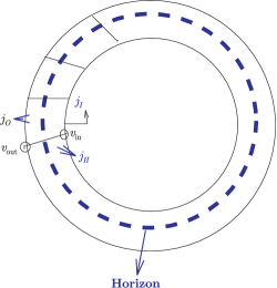
Figure 1: Graph at the horizon.

We then further concentrate on two vertices $v_{\rm out}$ outside the horizon, $v_{\rm in}$ inside the horizon which share a radial edge $e_{H}$ and write a density matrix for that $\rho^{\rm local}$. At each vertex $v_{\rm out,in}$ there are two angular edges corresponding to the $\theta$, $\phi$ coordinate lines which are ingoing and two angular edges which are outgoing. These angular edges, 4 in number at each vertex have their classical $g_{e}$ correlated with those meeting at the other vertex. Labeling $\psi_{j}(g)_{mn}=\frac{1}{\langle\psi|\psi\rangle^{1/2}}e^{-t/2j(j+1)}\pi_{j}(g_{e})_{mn}$,

$$\rho^{\rm local}=\sum_{\{j_{Oi}\}\{j_{H}\}\{j_{Ii}\},\{j^{\prime}_{Oi}\}\{j^{\prime}_{H}\}\{j^{\prime}_{Ii}\}}\prod_{i=1}^{4}\psi_{j_{Oi}}(g_{e}(v_{\rm out})[g_{e}(v_{\rm in})])_{m_{Oi}n_{Oi}}\psi_{j_{H}}(g_{e_{H}})_{m_{H}n_{H}}$$

$$\phantom{\rho^{\rm local}=}\times\prod_{i=1}^{4}\psi_{j_{Ii}}(g_{e}(v_{\rm in}))_{m_{Ii}n_{Ii}}\prod_{i=1}^{4}|\{j_{Oi}\}\{j_{H}\}\{j_{Ii}\}\rangle\langle\{j^{\prime}_{Oi}\}\{j^{\prime}_{H}\}\{j^{\prime}_{Ii}\}|$$

$$\phantom{\rho^{\rm local}=}\times\prod_{i=1}^{4}\bar{\psi}_{j^{\prime}_{Oi}}(g_{e}(v_{\rm out})[g_{e}(v_{\rm in})])_{m^{\prime}_{Oi}n^{\prime}_{Oi}}\psi_{j^{\prime}_{H}}(g_{e_{H}})_{m^{\prime}_{H}n^{\prime}_{H}}\prod_{i=1}^{4}\bar{\psi}_{j^{\prime}_{Ii}}(g_{e}(v_{\rm in}))_{m^{\prime}_{Ii}n^{\prime}_{Ii}}.$$

$j_{Oi}m_{0i}n_{0i}$ label the spins of the edges at the outside vertex. $j_{Ii}m_{Ii}n_{Ii}$ label the spins at the inner vertex and the $j_{H}$, $m_{H}$, $n_{H}$ label the spins on the radial edge connecting the two vertices. We us $\{j\}$ to label all the three indices $jmn$. The tracing over the modes inside the horizon gives in the $t\rightarrow 0$ limit

$$\rho^{\rm local}_{\rm reduced}=\sum_{\{j_{Oi}\}\{j_{H}\}\{j_{Ii}\}\{j^{\prime}_{Oi}\}\{j_{H}^{\prime}\}}\prod_{i=1}^{4}\psi_{j_{Oi}}(g_{e}(v_{\rm out})(g_{e}(v_{\rm in})))_{m_{Oi}n_{Oi}}\psi_{j_{H}}(g_{e_{H}})_{m_{H}n_{H}}$$

$$\phantom{\rho^{\rm local}_{\rm reduced}=}\times\prod_{i=1}^{4}\delta(P_{e_{i}}(v_{\rm in}),j_{Ii}t)|\{j_{Oi}\}\{j_{H}\}\rangle\langle\{j^{\prime}_{Oi}\}\{j^{\prime}_{H}\}|\bar{\psi}_{j^{\prime}_{H}}(g_{e_{H}})_{m^{\prime}_{H}n^{\prime}_{H}}$$

$$\phantom{\rho^{\rm local}_{\rm reduced}=}\times\prod_{j^{\prime}_{i}=1}^{4}\bar{\psi}_{j^{\prime}_{Oi}}(g_{e}(v_{\rm out})[g_{e}(v_{\rm in})])_{m^{\prime}_{Oi}n^{\prime}_{Oi}}.$$

In the $t\rightarrow 0$ limit, the diagonal terms dominate. The density matrix collapses to a set of non-zero elements [42]. This can be directly seen from

$$\frac{1}{\langle\psi|\psi\rangle}e^{-tj(j+1)}\pi_{j}(\bar{g})_{mn}\pi_{j}(g)_{mn}$$

$$\qquad\approx\frac{t^{3/2}}{4\sqrt{\pi}p}e^{-jp|m/j-(^{R}p)_{3}/p|}e^{-jp|n/j-(^{L}p)_{3}/p|}e^{-[(j+1/2)-p]^{2}/t}.$$ (4.8)

In the $t\rightarrow 0$ limit, this gets to be peaked like a delta function at the values $P=(j+1/2)t$, $mt,nt={}^{L}P_{3},{}^{R}P_{3}$ are the left and right invariant momentum operators. As in [18] the $j_{Oi}$ gets fixed to be a certain number due to the apparent horizon equation (4.6), and the corresponding $m_{Oi}$, $n_{Oi}$ were also taken as fixed numbers using a ‘gauge fixed’ version of the apparent horizon equation. However this is slightly arbitrary as the classical data is gauge invariant. We expect that when all the constraints including the Gauss constraints are solved this will emerge as obvious.

The individual components of ${}^{L(R)}\hat{P}^{3}_{e_{Oi}}$, fixes the $m_{0i}n_{0i}$ to unique numbers. Thus the outer classical data $j^{\rm cl}_{Oi}$, $m^{\rm cl}_{Oi}$, $n^{\rm cl}_{Oi}$ have to be specified completely to specify the ‘outer state’. In other words we can break the degeneracy of the density matrix with different $m_{Oi}n_{Oi}$ by making the operator measurements.

Now we come to a subtle point I had not discussed before, and that is the fact that the part of the radial edge $e_{H}$ (see Fig. 1) is hidden behind the horizon. It thus makes sense to trace over that. To implement that, we therefore divide the horizon edge $e_{H}$ into two further edges $e_{H1}$ and $e_{H2}$. We build the basis state for this using the fact that

$$|jmn\rangle=\sqrt{2j+1}\pi_{j}(h_{e})_{mn}|0\rangle$$

$$\hphantom{|jmn\rangle}{}=\sum_{k}\sqrt{2j+1}\pi_{j}(h_{e_{1}})_{mk}\pi_{j}(h_{e_{2}})_{kn}|0\rangle=\sum_{k}\frac{1}{\sqrt{2j+1}}|jmk\rangle|jkn\rangle,$$

where $|0\rangle$ is the vacuum state. Splitting the horizon edge, and tracing over the internal half gives

$$\operatorname{Tr}{e_{2}}|jmn\rangle\langle j^{\prime}m^{\prime}n^{\prime}|=\sum_{k^{\prime}kn}\frac{1}{2j+1}|j^{\prime}m^{\prime}k\rangle\langle j^{\prime}k^{\prime}n^{\prime}|jkn\rangle\langle j^{\prime}m^{\prime}k^{\prime}|$$

$$\phantom{\operatorname{Tr}{e_{2}}|jmn\rangle\langle j^{\prime}m^{\prime}n^{\prime}|}=\sum_{k}\frac{1}{2j+1}|jmk\rangle\langle jm^{\prime}k|\delta_{nn^{\prime}}.$$ (4.9)

Similarly, for the irreducible representation components of the ‘wavefunction’

$$\pi_{j}(g_{e})_{mn}\bar{\pi}_{j}(g_{e})_{m^{\prime}n},$$

which multiplies the basis states in the density matrix, one can perform such a splitting of the holonomy as

$$g_{e}=e^{iT^{I}P^{I}}h_{e}=e^{iT^{I}P^{I}}h_{e_{1}}h_{e_{2}}=g_{e_{1}}h_{e_{2}},$$

and thus

$$\sum_{kk^{\prime}}\pi_{j}(g_{e_{1}})_{mk}\pi_{j}(h_{e_{2}})_{kn}\bar{\pi}_{j}(g_{e_{1}})_{m^{\prime}k^{\prime}}\bar{\pi}_{j}(h_{e_{2}})_{k^{\prime}n}.$$

The sum over $n$ then gives

$$\pi_{j}(g_{e_{1}})_{mk}\bar{\pi}_{j}(g_{e})_{m^{\prime}k}=\pi\big{(}e^{\iota T^{I}P^{I}}\big{)}_{mm^{\prime}}.$$ (4.10)

This and then its complex conjugate gives the delta function in the $t\rightarrow 0$ limit peaked at $P_{H}$. The contribution from the horizon edge to the density matrix is

$$\frac{1}{2j_{H}+1}\sum_{m_{H}k_{H}}\delta(j_{H}t,P_{e_{H}})|j_{H}m_{H}k_{H}\rangle\langle j_{H}m_{H}k_{H}|.$$

This explains the origin of the $1/(2j_{H}+1)$ factor anticipated in [18].

Thus the reduced density matrix ‘describing the vertex outside the horizon’ is

$$\mathop{\rm Lim}\limits_{t\rightarrow 0}\rho^{\rm local}_{{\rm reduced}}=\sum_{m_{H}n_{H}}\frac{1}{2j_{H}+1}$$

$$\hphantom{\mathop{\rm Lim}\limits_{t\rightarrow 0}\rho^{\rm local}_{{\rm reduced}}=}\times\prod_{i=1}^{4}|P_{e_{Oi}},{}^{L}p_{3Oi}\,{}^{R}p_{3Oi}\rangle|P_{e_{H}}m_{H}n_{H}\rangle\langle P_{e_{H}}m_{H}n_{H}|\langle P_{e_{Oi}},{}^{L}p_{3Oi}\,{}^{R}p_{3Oi}|.$$

And the tensor product density matrix becomes

$$\rho^{\rm local}_{\rm reduced}=\prod_{v_{\rm out}}\sum_{m_{H}n_{H}}\frac{1}{2j_{H}+1}$$

$$\phantom{\rho^{\rm local}_{\rm reduced}=}\times\prod_{i=1}^{4}|P_{e_{Oi}},{}^{L}p_{3Oi}\,{}^{R}p_{3Oi}\rangle|P_{e_{H}}m_{H}n_{H}\rangle\langle P_{e_{H}}m_{H}n_{H}|\langle P_{e_{Oi}},{}^{L}p_{3Oi}\,{}^{R}p_{3Oi}|,$$

the above density matrix is clearly diagonal. If we then compute

$$-\operatorname{Tr}(\rho^{\rm local}_{\rm reduced}\ln\rho^{\rm local}_{\rm reduced})=\frac{\beta A_{\rm BH}}{4l_{p}^{2}}+{\rm corrections},$$

where $\beta$ is a prefactor [19]. The exact computation is not obvious, but if we assume that every $j_{H}$ is the same, then this gives $-\operatorname{Tr}\big{(}\rho^{\rm local}_{\rm reduced}\ln\rho^{\rm local}_{\rm reduced}\big{)}=\sum_{v_{\rm out}}\ln(2j_{H}+1)=A_{H}\ln(2j_{H}+1)/[l_{p}^{2}(j_{H}+1/2)]$ where we used the constraint (4.7) such that the $\sum(j_{H}+1/2)=A_{H}/l_{p}^{2}$. For different distribution of spins one has to use combinatorics [18, 19].

Thus to leading order the entropy as computed from the density matrix is indeed Bekenstein–Hawking modulo the $\beta$ which is a function of the Immirzi parameter and other details of the combinatorics of the graph can be set to 1.

4.2 Quantum correlations

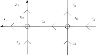
Figure 2: Spins at the vertices.

We now discuss the correlations across the horizon due to intertwiners placed at the vertices. As evident the coherent states are defined in a ${\rm SU}(2)$ Hilbert space. For the holonomy variables, the ${\rm SU}(2)$ gauge transformations act at the beginning and end point of the edges. $h_{e}\rightarrow g^{-1}(v_{1})h_{e}(v_{1},v_{2})g(v_{2})$. These changes will change the spin network state. To make the state gauge invariant one imposes intertwiners at the vertices. These are structures which map the spin networks at the vertex to the trivial representation. Thus the state does not transform due to the intertwiners. We concentrate on two vertices (suppress one dimension) and take each vertex to be four valent at the horizon and observe the role of the intertwiners. From the Fig. 2 two of the edges are ingoing, the other two are outgoing at each vertex. The gauge transformations act on the holonomies and hence the basis states on each edge at the vertices. Integrating (group averaging) over the gauge group at the vertices, one ensures gauge invariance [41, 22, 21]. This solves the Gauss constraint. We find that when done carefully this gives us correlations between the coherent state at inner and outer vertices which are carried by the horizon edge which connects the two vertices. This is therefore a ‘quantum correlation’. We describe some of the details of the calculations here. Let us take the two vertices as $v_{\rm in}$ and $v_{\rm out}$ and the spin labels $j_{I1}$, $j_{I2}$, $j_{I3}$, $j_{H}$ at the inner vertex and $j_{O1}$, $j_{O2}$, $j_{O3}$, $j_{H}$ at the outer vertex. Let us assume that at the inner vertex $j_{I1}$, $j_{H}$ are outgoing at that vertex, or they ‘begin’ at $v_{\rm in}$ and the $j_{I2}$, $j_{I3}$ are ingoing at the vertex or have their end point at that vertex. Similarly at the outer vertex, $j_{H}$ and $j_{O3}$ are ingoing or end at $v_{\rm out}$ and $j_{O1}$, $j_{O2}$ are outgoing and begin at the vertex $v_{\rm out}$. To introduce the intertwiners we observe the basis spin network functions and their transformations. The basis spin network states $|jmn\rangle$ at the inner vertex in the $h_{e}$ representation are given as ($\sqrt{2j+1}$ factor is not shown but it exists in each basis state for normalisation of the inner product)

$$\pi_{j_{I1}}(h)_{m_{I1}n_{I1}}\pi_{j_{I2}}(h)_{m_{I2}n_{I2}}\pi_{j_{I3}}(h)_{m_{I3}n_{I3}}\pi_{j_{H}}(h)_{m_{H}n_{H}},$$

the gauge action $U(g)$ at the vertex is such that

$$\pi_{j_{I1}}(gh)_{m_{I1}n_{I1}}\pi_{j_{I2}}\big{(}hg^{-1}\big{)}_{m_{I2}n_{I2}}\pi_{j_{I3}}\big{(}hg^{-1}\big{)}_{m_{I3}n_{I3}}\pi_{j_{H}}(gh)_{m_{H}n_{H}}.$$

Upon group averaging one obtains a projector onto the gauge invariant Hilbert space which written using the $3jm$ symbols is thus (see Appendix A for further details)

$$\sum_{\{j_{k}\}p_{I1}q_{I2}q_{I3}p_{H}}(2j_{k}+1)\left(\begin{matrix}{j_{I1}}&j_{H}&j_{k}\\ m_{I1}&m_{H}&m_{k}\end{matrix}\right)\left(\begin{matrix}j_{I1}&j_{H}&j_{k}\\ p_{I1}&p_{H}&n_{k}\end{matrix}\right)$$

$$\qquad{}\times\overline{\left(\begin{matrix}j_{I2}&j_{I3}&j_{k}\\ n_{I2}&n_{I3}&m_{k}\end{matrix}\right)}\overline{\left(\begin{matrix}j_{I2}&j_{I3}&j_{k}\\ q_{I2}&q_{I3}&n_{k}\end{matrix}\right)}$$

$$\qquad{}\times\pi_{j_{I1}}(h)_{p_{I1}n_{I1}}\pi_{j_{I2}}(h)_{m_{I2}q_{I2}}\pi_{j_{I3}}(h)_{m_{I3}q_{I3}}\pi_{j_{H}}(h)_{p_{H}n_{H}}.$$ (4.11)

We can then collect the basis vectors and the $3jm$ symbols contracted with them as a $|\rm in\rangle$ basis

$$=\sum_{\{j_{k}\}}\left(\begin{matrix}{j_{I1}}&j_{H}&j_{k}\\ m_{I1}&m_{H}&m_{k}\end{matrix}\right)\overline{\left(\begin{matrix}{j_{I2}}&j_{I3}&j_{k}\\ n_{I2}&n_{I3}&m_{k}\end{matrix}\right)}|{\rm in}\rangle.$$

If we take $\psi_{j}(g_{e})_{mn}=\frac{1}{\langle\psi|\psi\rangle}e^{-t/2j(j+1)}\pi_{j}(g_{e})_{mn}$, the coherent state wavefunction at the inner vertex is

$$\sum_{\{j\}}\prod_{i=1}^{3}\psi_{j_{Ii}}(g_{e_{Ii}})_{m_{Ii}n_{Ii}}\left(\begin{matrix}{j_{I1}}&j_{H}&j_{k}\\ m_{I1}&m_{H}&m_{k}\end{matrix}\right)\overline{\left(\begin{matrix}{j_{I2}}&j_{I3}&j_{k}\\ n_{I2}&n_{I3}&m_{k}\end{matrix}\right)}|\rm in\rangle.$$

Note that this way, only the indices which begin or end at the $v_{\rm in}$ are gauge invariant, the other end of the edges remains ‘free’ and can be attached to another vertex in an invariant way. Exactly in the same way one can obtain the gauge invariant wavefunction at the outer vertex, comprising of the $3jm$ symbols and the corresponding wavefunctions. And therefore one can define the intertwiners at the outer vertex but notice immediately the horizon edge is shared by both the outer vertex and the innner vertex, and thus, the correct way to write the coherent state for the edges meeting at the two vertices is this

$$|\psi(v_{\rm out},v_{\rm in})\rangle=\sum_{\{j\}}\Psi(\{j_{0i}\},\{j_{H}\},\{j_{Ii}\})|{\rm out}\rangle|H\rangle|{\rm in}\rangle,$$

where $|H\rangle$ is the horizon state for the horizon edge crossing the horizon (see Fig. 1). Clearly the coefficient of the basis states do not factorise and can be identified as

$$\Psi(\{j_{0i}\},\{j_{H}\},\{j_{Ii}\})=\prod_{i=1}^{3}\psi_{j_{Oi}}(g_{e_{Oi}})_{m_{Oi}n_{Oi}}\sum_{\tilde{j}_{k}^{\prime}}\left(\begin{matrix}j_{01}&j_{O2}&{\tilde{j}_{k}^{\prime}}\\ m_{O1}&m_{O2}&{\tilde{m}_{k}^{\prime}}\end{matrix}\right)$$

$$\phantom{\Psi(\{j_{0i}\},\{j_{H}\},\{j_{Ii}\})=}\times\overline{\left(\begin{matrix}{\tilde{j}_{k^{\prime}}}&j_{O3}&j_{H}\\ {\tilde{m}}_{k^{\prime}}&n_{O3}&n_{k}\end{matrix}\right)}\psi_{j_{H}}(g_{e_{H}})_{m_{H}n_{H}}$$

$$\phantom{\Psi(\{j_{0i}\},\{j_{H}\},\{j_{Ii}\})=}\times\sum_{j_{k}}\prod_{i=1}^{3}\psi_{j_{Ii}}(g_{e_{Ii}})_{m_{Ii}n_{Ii}}\left(\begin{matrix}{j_{I1}}&j_{H}&j_{k}\\ m_{I1}&m_{H}&m_{k}\end{matrix}\right)\overline{\left(\begin{matrix}{j_{I2}}&j_{I3}&j_{k}\\ n_{I2}&n_{I3}&m_{k}\end{matrix}\right)}.$$

The density matrix is then

$$\rho_{\rm inv}=|\psi(v_{\rm out},v_{\rm in})\rangle\langle\psi(v_{\rm out},v_{\rm in})|.$$

This in a very sure way establishes that correlations exist across the horizon surface, the question however is that is Bekenstein–Hawking entropy recovered from the tracing mechanism as previously? Ab initio it is not expected that this will happen, as these gauge invariant coherent states do not have the appropriate peakedness properties of the gauge non-invariant coherent states [42]. We simply implement the tracing of the inner edges to find the reduced density matrix at this stage and demonstrate the entanglement.

The reduced density matrix is easily obtained, using the trace over the inner basis states and some $3jm$ symbol identities (see Appendix A). The matrix elements turn out to be

$$\sum_{\{j_{Ii}\}}\Psi\left(\{j_{Oi}\},\{j_{H}\},\{j_{Ii}\})\bar{\Psi}(\{j^{\prime}_{Ii}\},\{j^{\prime}_{H}\},\{j_{Oi}\}\right)$$

$$\qquad{}=\Psi(\{j_{0i}\},\{j_{H}\})\bar{\Psi}(\{j^{\prime}_{H}\},\{j^{\prime}_{Oi}\})\sum_{\{j_{Ii}\},j_{k}}\frac{(2j_{k}+1)\delta(j_{I1}j_{H}j_{k})\delta(j_{k}j_{I2}j_{I3})}{(2j_{H}+1)}$$

$$\qquad\quad{}\times\prod_{i=1}^{3}\psi_{j_{Ii}}(g_{e_{Ii}})_{m_{Ii}n_{Ii}}\prod_{i=1}^{3}\bar{\psi}_{j_{Ii}}(g_{e_{Ii}})_{m^{\prime}_{Ii}n^{\prime}_{Ii}}\delta_{n^{\prime}_{I1}n_{I1}}\delta_{m^{\prime}_{I2}m_{I2}}\delta_{m^{\prime}_{I3}m_{I3}}$$

$$\qquad\quad{}\times\left(\begin{matrix}{j_{I1}}&j_{H}&j_{k}\\ m_{I1}&m_{H}&m_{k}\end{matrix}\right)\left(\begin{matrix}{j_{k}}&j_{I2}&j_{I3}\\ m_{k}&n_{I2}&n_{I3}\end{matrix}\right)\left(\begin{matrix}{j_{I1}}&j_{H}&j_{k}\\ m^{\prime}_{I1}&m^{\prime}_{H}&m^{\prime}_{k}\end{matrix}\right)\left(\begin{matrix}{j_{k}}&j_{I2}&j_{I3}\\ m^{\prime}_{k}&n^{\prime}_{I2}&n^{\prime}_{I3}\end{matrix}\right).\!\!\!\!$$ (4.12)

Whereas it is not obvious what this will yield for the entropy which is $S_{\rm BH}=-\operatorname{Tr}(\rho\ln\rho)$, one can use the fact that again in the limit that $t\rightarrow 0$, the product of wavefunctions will assume the form in equation (4.8)

$$\sum_{\{j_{i}\}}\Psi\left(j_{Oi},j_{H},j_{Ii})\bar{\Psi}(j_{Ii},j^{\prime}_{H},j^{\prime}_{Oi}\right)=\Psi(j_{0i},j_{H})\bar{\Psi}(j^{\prime}_{H},j^{\prime}_{Oi})\sum_{j_{k}}\frac{(2j_{k}+1)\delta(j_{I1}j_{H}j_{k})\delta(j_{k}j_{I2}j_{I3})}{(2j_{H}+1)}$$

$$\qquad{}\times\left(\begin{matrix}{j^{\rm cl}_{I1}}&j_{H}&j_{k}\\ m^{\rm cl}_{I1}&m_{H}&m_{k}\end{matrix}\right)\left(\begin{matrix}{j_{k}}&j^{\rm cl}_{I2}&j^{\rm cl}_{I3}\\ m_{k}&n^{\rm cl}_{I2}&n^{\rm cl}_{I3}\end{matrix}\right)\left(\begin{matrix}{j^{\rm cl}_{I1}}&j_{H}&j_{k}\\ m^{\rm cl}_{I1}&m^{\prime}_{H}&m^{\prime}_{k}\end{matrix}\right)\left(\begin{matrix}{j_{k}}&j^{\rm cl}_{I2}&j^{\rm cl}_{I3}\\ m^{\prime}_{k}&n^{\rm cl}_{I2}&n^{\rm cl}_{I3}\end{matrix}\right).$$

The above reduced density matrix is precisely of the form expected to yield the entropy, but the $3jm$ symbols are non-trivial and one can use some asymptotic form given in [35] for large $j$ to estimate the form of the density matrix. Details of this calculations and further computations of the entropy will appear in [15]. This is the absolute proof of the fact that the coherent state introduced to describe the black hole is entangled across the horizon and does not factorise into inside and outside coefficients. There has been work in observing entanglement in semiclassical states independently as in [30].

5 Time evolution

In this section we discuss time evolution of the system. Fortunately as the system is semiclassical, a natural choice of time is the asymtotic time coordinate. Using the Lemaitre slice and evolving the state in Lemaitre time would not serve the purpose as that is the frame of an infalling observer. We use the frame of an observer stationed outside the horizon to evolve the slice in her time as at the asymptotics this coincides with Minkowski time. Again we concentrate on the evolution of a local patch surrounding the horizon. Normally the vertices within the horizon are classically forbidden to the outside observer. However we allow for access to those vertices in the ‘quantum mechanical’ evolution. The ‘Hamiltonian’ which is used to evolve the horizon is the Brown and York quasi-local energy.

5.1 Semi classical Hamiltonian

Quasi-local Hamiltonian is defined as the energy enclosed in a finite space. This is obtained using a particular definition [13], as the ‘surface’ integral of the extrinsic curvature with which the surface is embedded in three space. This generates time translation in the timelines orthogonal to the spatial slice. In our case, we take the bounding surface to be the horizon and the quasilocal energy is given by the surface term [13, 28]

$$\tilde{H}=\frac{1}{\kappa}\int d^{2}x\sqrt{\sigma}k,$$

where $k$ is the extrinsic curvature with which the 2-surface, which in this case is the horizon $S^{2}$ embedded in the spatial 3-slices, and $\sigma$ is the determinant of the two metric $\sigma_{\mu\nu}$ defined on the 2-surface. This ‘quasilocal energy’ is measured with reference to a background metric. Thus $H=\tilde{H}-H_{0}$ where $H_{0}$ is the energy in the background. We concentrate on the physics observed by an observer stationed at a $r={\rm const}$ sphere.

The metric in static $r={\rm const}$ observer’s frame is

$$ds^{2}=-f^{2}dt^{2}+r^{2}\big{(}d\theta^{2}+\sin^{2}\theta d\phi^{2}\big{)},$$

$f=\sqrt{1-r_{g}/r}$, where $r_{g}$ is the Schwarzschild radius. If we take $n_{\mu}$ to be the space-like vector, normal to the 2-surface, then the extrinsic curvature is given by $k_{\mu\nu}=\sigma_{\mu}^{\alpha}\nabla_{\alpha}n_{\nu}$ and the trace is obviously

$$k=\nabla^{\alpha}n_{\alpha}.$$ (5.1)

In the special slicing of the stationary observer the normal to the horizon 2-surface is given by $(0,f(r),0,0)$. However, we built the density matrix on the Lemaitre slice. The Lemaitre and the Schwarzschild observer’s coordinates are related by the following coordinate transformations

$$\sqrt{\frac{r}{r_{g}}}dr=(dR-d\tau),\qquad dt=\frac{1}{1-f^{\prime}}\left(d\tau-f^{\prime}dR\right),\qquad f^{\prime}=\frac{r_{g}}{r}.$$

The $r={\rm const}$ cylinder of the Schwarzschild coordinate corresponds to $dR=d\tau$ of the Lemaitre coordinates, and for these $dt=d\tau$. Thus unit translation in the $t$ coordinate coincides with unit translation in the $\tau$ coordinate. Further, the intersection of the $r={\rm const}$ cylinder with a $t={\rm const}$ surface coincides with the intersection of $r={\rm const}$ and the $\tau={\rm const}$ surface. Thus in the initial slice, the QLE Hamiltonian can be written in terms of the Christoffel symbols of the Lemaitre slice. Even though the generic transformation of the Christoffel symbols from one coordinate frame to the other is inhomogeneous, in this example, the transformation is trivial. The trace of the extrinsic curvature (5.1) then written using Christoffel symbols turns out to be

$$H=\frac{1}{2\kappa}\int d\theta d\phi\sqrt{g_{\theta\theta}g_{\phi\phi}}\left[-g^{\theta\theta}\frac{\partial g_{\theta\theta}}{\partial r}-g^{\phi\phi}\frac{\partial g_{\phi\phi}}{\partial r}\right]f(r)-H_{0}.$$ (5.2)

The reference frames’ quasilocal energy $H_{0}$ is a number, it just defines the zero point Hamiltonian. Thus, we replace the classical expressions by operators evaluated at the $\tau={\rm const}$ slice. In the first approximation we simply take the $f(r)$ as classical $\sqrt{1-r_{g}/r}=\sqrt{\delta_{e_{r}}/2r_{g}}=\epsilon$, as this arises due to the coordinate transformation and the norm of the vector $n_{r}$ in the previous frame. In the re-writing of (5.2) in regularised LQG variables the Hamiltonian appears rather complicated.

One can rewrite these in a much simpler form, using the apparent horizon equation. Since the Hamiltonian is an integral over the horizon, the variables will satisfy the apparent horizon equation (4.2) up to quantum fluctuations. Thus the Hamiltonian operator is then re-written as

$$H_{\rm horizon}=\frac{\epsilon}{\kappa}\int d\theta d\phi\sqrt{g_{\theta\theta}g_{\phi\phi}}\big{[}K^{I}_{\theta}e^{I\theta}+K^{I}_{\phi}e^{I\phi}\big{]},$$

where we have used the classical apparent horizon equation (4.2) (with $q^{rr}=1$). The regularised LQG version of this is

$$H_{\rm horizon}=\frac{Ca~{}\epsilon}{2\kappa\delta_{e_{\theta}}s_{e_{\theta}}}\sum_{v_{\rm out}}\operatorname{Tr}\left[h_{e_{\theta}}^{-1}T^{I}\beta\frac{\partial}{\partial\beta}h_{e_{\theta}}\right]P_{e_{\theta}}^{I}+\text{h.c.}+(\theta\rightarrow\phi),$$ (5.3)

where $C$ consists of some dimensionless constants $s_{e_{\theta}}$ is the 2-dimensional area bit over which $E^{\theta}_{I}$ is smeared, $a$ is a dimensionfull constant which appears to get the $P_{e_{\theta}}^{I}$ dimension less. $\delta_{e_{\theta}}$ is the length for the angular edge $e_{\theta}$ over which the gauge connection is integrated to obtain the holonomy. The sum over $v_{\rm out}$ is the set of vertices immediately outside the horizon. The (5.3) can then be lifted to an operator. However, this Hermitian operator gives no change to horizon entropy as the coherent state is evolved from one time slice to the next. Surprisingly a non-Hermitian term evolves the slices non-trivially. These anti-Hermitian terms can be easily found in this formalism if we allow for the vertices within the horizon to be exposed to the outside observer. In this case as the region is within the classical horizon, the norm of the Killing vector is negative, and $n_{r}$ has components which are imaginary. The $\epsilon\rightarrow\pm\iota\epsilon$. One sees why the inner vertices are relevant in a semiclassical evolution even if they are classically forbidden: In quantum mechanics tunneling is a well known phenomena, and inclusion of the inner vertices facilitates the process.

Thus the contribution of ‘inner vertices’ $v_{\rm in}$ is added to the Hamiltonian and it gives the anti-Hermitian contribution to the Hamiltonian. Thus $H_{\rm horizon}=\frac{1}{2}\big{[}\sum_{v_{\rm out}}H_{v_{\rm out}}+\sum_{v_{\rm in}}H_{v_{\rm in}}\big{]}$. The regularised Hamiltonian is not Hermitian, and the evolution equation is

$$\iota\hbar\frac{\partial\rho}{\partial\tau}=H\rho-\rho H^{{\dagger}}.$$ (5.4)

Thus one takes the evolved slice to have a density matrix

$$\rho=\rho^{0}-\frac{\iota\delta\tau}{\hbar}\big{[}H\rho^{0}-\rho^{0}H^{{\dagger}}\big{]}.$$

The entropy computed using this density matrix is different from the entropy in the previous slice and the difference of entropy can be seen as obtained using a simplified model.

Let the density matrix be defined for a system whose states are given in the tensor product Hilbert spaces $H_{1}\otimes H_{2}$ and given by

$$|\psi\rangle=\sum_{ij}d_{ij}|i\rangle|j\rangle,$$

where $|i\rangle$ is the basis in $H_{1}$ and $|j\rangle$ is the basis in $H_{2}$ and $d_{ij}$ are the non-factorisable coefficients of the wavefunction in this basis. Let us label the wavefunction at time $t=0$ to be given by the coefficients $d^{0}_{ij}$. The density matrix is

$$\rho^{0}=\sum_{iji^{\prime}j^{\prime}}d^{0*}_{i^{\prime}j^{\prime}}d^{0}_{ij}|i\rangle|j\rangle\langle j^{\prime}|\langle i^{\prime}|.$$

The reduced density matrix if one traces over $H_{2}$ is

$$\operatorname{Tr}_{2}\rho^{0}=\sum_{ii^{\prime}}\sum_{j}d^{0*}_{i^{\prime}j}d^{0}_{ij}|i\rangle\langle i^{\prime}|.$$

We now evolve the system using a Hamiltonian which has the matrix elements $H_{iji^{\prime}j^{\prime}}|i\rangle|j\rangle\langle j^{\prime}|\langle i^{\prime}|$, we assume that the Hamiltonian does not factorise, that is there exists interaction terms between the two Hilbert spaces. The evolution equation is

$$i\hbar\frac{\partial\rho}{\partial\tau}=[H,\rho],$$

which in this particular basis gives the density matrix elements at an infinitesimally nearby slice to be

$$d^{\delta\tau*}_{i^{\prime}j^{\prime}}d^{\delta\tau}_{ij}=d^{0*}_{i^{\prime}j^{\prime}}d^{0}_{ij}-\frac{i}{\hbar}\delta\tau\left[\sum_{kl}\left(H_{ijkl}d^{0}_{kl}d^{0*}_{i^{\prime}j^{\prime}}-d^{0}_{ij}d^{0*}_{kl}H_{kli^{\prime}j^{\prime}}\right)\right].$$

Thus we evolve the ‘unreduced’ density matrix and then trace over the $H_{2}$ in the evolved slice. The reduced density matrix in the evolved slice is

$$\sum_{j}d^{\delta\tau*}_{i^{\prime}j}d^{\delta\tau}_{ij}=\sum_{j}d^{0*}_{i^{\prime}j}d^{0}_{ij}-\frac{i}{\hbar}\delta\tau\left[\sum_{klj}\left(H_{ijkl}d^{0}_{kl}d^{0*}_{i^{\prime}j}-d^{0}_{ij}d^{0*}_{kl}H_{kli^{\prime}j}\right)\right].$$

This gives

$$\rho^{\delta\tau}=\rho^{0}-\frac{i}{\hbar}\delta\tau A,$$

where $A$ represents the commutator. Clearly the entropy in the evolved slice evaluated as $S_{\rm BH}^{\delta\tau}=-\operatorname{Tr}(\rho\ln\rho)$ can be found as

$$S_{\rm BH}^{\delta\tau}=S_{\rm BH}^{0}+\frac{i}{\hbar}\delta\tau\big{[}\operatorname{Tr}A\ln\rho^{0}+\operatorname{Tr}\rho^{0}\rho^{0\ -1}A\big{]}.$$

Given the definition of $A_{ii}$, one gets

$$A_{ii}=\sum_{jkl}\left[\rho^{0}_{ijkl}H_{klij}-H_{ijkl}\rho^{0}_{klij}\right].$$

In case both the Hamiltonian and the density operator are Hermitian, one obtains

$$\sum_{j}A_{jj}=2\iota\operatorname{Im}\operatorname{Tr}\big{(}\rho^{0}H\big{)}.$$

This is clearly calculable, and gives the change in entropy $\Delta S_{\rm BH}$. The $\ln\rho^{0}$ term yields corrections, and we ignore it in the first approximation. However if the Hamiltonian is non-Hermitian one gets

$$\Delta S_{\rm BH}=\frac{\iota\delta\tau}{\hbar}{\rm Tr}\big{[}H\rho^{0}-\rho^{0}H^{{\dagger}}\big{]}$$ (5.5)

instead of the commutator.

In case of the gravitational Hamiltonian, the above can be computed using a ${\rm U}(1)$ projection thus. Let us take the ${\rm U}(1)$ case to make the calculations easier and observe the action of the Hamiltonian on the evolution of the coherent state. The spin network states are replaced by $|n\rangle=e^{\iota n\zeta}$, $0<\zeta<2\pi$, $n$ is an integer and the coherent states are

$$\psi^{t}(g_{e})=\sum_{n}e^{-(tn^{2})/2}e^{in(\chi_{e}-ip_{e})}e^{-\iota n\zeta}.$$

$g_{ne}=e^{in(\chi_{e}-ip_{e})}$ is the complexified phase space element in the ‘$n$th’ representation.

The quasi local energy operator (5.3) also takes the simplified form

$$H_{\rm horizon}^{\rm U(1)}=-\frac{1}{2}C^{\prime}\iota\hat{h}_{e}^{-1}\beta\frac{\partial}{\partial\beta}\hat{h}_{e}\hat{p}_{e}+\frac{1}{2}C^{\prime}\iota\hat{p}_{e}\beta\frac{\partial\hat{h}_{e}^{-1}}{\partial\beta}\hat{h}_{e}.$$ (5.6)

The prefactors have been clubbed into $C^{\prime}$. The U(1) coherent states are eigenstates of an annihilation operator defined thus:

$$\hat{g}_{e}=e^{t/2}e^{\hat{p}_{e}}\hat{h}_{e},\qquad\hat{g}_{e}|\psi\rangle=g_{e}|\psi\rangle.$$

The holonomy operator can thus be written as

$$\hat{h}_{e}=e^{-t/2}e^{-\hat{p}_{e}}\hat{g}_{e}.$$

And the derivative w.r.t. Immirzi parameter of the holonomy which appears in the definition of the Hamiltonian replaced by

$$\beta\frac{\partial\hat{h}_{e}}{\partial\beta}=e^{-t/2}\left[-\beta\frac{\partial\hat{p}}{\partial\beta}e^{-\hat{p}_{e}}\hat{g}_{e}+e^{-\hat{p}_{e}}\beta\frac{\partial\hat{g}_{e}}{\partial\beta}\right]=e^{-t/2}\left[\hat{p}_{e}e^{-p_{e}}\hat{g}_{e}+e^{-\hat{p}}\beta\frac{\partial\hat{g}_{e}}{\partial\beta}\right].$$

The dependence of the operator $p$ on the Immirzi parameter is known (2.2), and thus we could evaluate the derivative ($\beta\partial_{\beta}p_{e}(\beta)=\beta\partial_{\beta}(p_{e}(1)/\beta)=-p_{e}(\beta)$).

The term

$$\operatorname{Tr}\big{(}\rho^{0}H^{\rm U(1)}_{\rm horizon}\big{)}$$ (5.7)

is then computable. Let us take the first term of (5.6) and find (5.7). As $\rho^{0}=|\psi\rangle\langle\psi|$, (5.7) gives simply (we drop the ‘$e$’ label for brevity)

$$\langle\psi|H^{\rm U(1)}_{\rm horizon}|\psi\rangle=\langle\psi|-\frac{1}{2}C^{\prime}\iota\hat{h}^{-1}\beta\frac{\partial}{\partial\beta}\hat{h}\hat{p}|\psi\rangle+\langle\psi|\text{h.c.}|\psi\rangle$$

$$\phantom{\langle\psi|H^{\rm U(1)}_{\rm horizon}|\psi\rangle}=-\frac{1}{2}\iota C^{\prime}\langle\psi|\hat{g}^{{\dagger}}e^{-t/2}e^{-\hat{p}}e^{-t/2}\left[\hat{p}\ e^{-\hat{p}}\hat{g}+e^{-\hat{p}}\beta\frac{\partial\hat{g}}{\partial\beta}\right]\hat{p}|\psi\rangle+\langle\psi|\text{h.c.}|\psi\rangle$$

$$\phantom{\langle\psi|H^{\rm U(1)}_{\rm horizon}|\psi\rangle}=-\frac{1}{2}\iota C^{\prime}e^{-t}g^{*}\left[\langle\psi|e^{-\hat{p}}\hat{p}e^{-\hat{p}}\hat{p}|\psi\rangle g+\langle\psi|e^{-2\hat{p}}\beta\frac{\partial\hat{g}}{\partial\beta}\hat{p}|\psi\rangle\right]+\langle\psi|\text{h.c.}|\psi\rangle.$$

We then concentrate on the 2nd term of the above

$$\langle\psi|e^{-2\hat{p}}\beta\frac{\partial\hat{g}}{\partial\beta}\hat{p}|\psi\rangle=\langle\psi|e^{-2\hat{p}}\beta\frac{\partial\hat{g}}{\partial\beta}\int\!d\nu(g^{\prime})|\psi^{\prime}\rangle\langle\psi^{\prime}|\hat{p}|\psi\rangle=\!\int\!d\nu(g^{\prime})\beta\frac{\partial g^{\prime}}{\partial\beta}\langle\psi|e^{-2\hat{p}}|\psi^{\prime}\rangle\langle\psi^{\prime}|\hat{p}|\psi\rangle,$$

where we have used the fact that coherent states resolve unity. It can be shown that the expectation value of the operators in the $t\rightarrow 0$ collapses the integral to $g^{\prime}=g$ point [42]. Thus one obtains from the above

$$\operatorname{Tr}\big{(}\rho^{0}H^{\rm U(1)}_{\rm horizon}\big{)}=-\frac{1}{2}\iota C^{\prime}e^{-t/2}\left[p+g^{*}e^{-2p}\beta\frac{\partial g}{\partial\beta}\right]p+\text{h.c.}=C^{\prime}\beta\frac{\partial\chi}{\partial\beta}p,$$ (5.8)

which is real, and thus

$$\Delta S_{\rm BH}=0$$

(this is actually the classical quasi local energy as it should be from $\operatorname{Tr}(\rho^{0}H_{\rm horizon})$).

This is obvious, as the way the Hamiltonian is defined, this is simply a function of the Hilbert space outside the horizon, and the matrix elements of this will not yield anything new. We approximated the horizon sphere by summing over $v_{1}$ vertices immediately outside the horizon. We could do the same by summing over $v_{2}$ vertices immediately within the horizon. For the Lemaitre slice, the metric is smooth at the horizon, and one can take the ‘quantum operators’ evaluated at the vertex $v_{2}$. In this case however, as the region is within the classical horizon, the norm of the Killing vector is negative, and $n_{r}$ has components which are imaginary. The $\epsilon\rightarrow\pm\iota\epsilon$. Thus $H_{\rm horizon}=\frac{1}{2}[\sum_{v_{1}}H_{v_{1}}+\sum_{v_{2}}H_{v_{2}}]$. In the evaluation of the quasi local energy term, the energy would emerge correct in the $\delta_{e_{r}}\rightarrow 0$ limit as $\epsilon\rightarrow 0$. The regularised Hamiltonian is not Hermitian, and the evolution equation is (5.4).

The same type of expectation or trace is obtained of the imaginary term (or $v_{2}$) is obtained as in (5.8), but this does not cancel in (5.5), and

$$\Delta S_{\rm BH}=\mp\frac{\delta\tau}{\hbar}C^{\prime}\beta\frac{\partial\chi}{\partial\beta}\ p.$$

The ‘rate of change’ of entropy is thus

$$\dot{\Delta}S_{\rm BH}=\mp\frac{\tilde{C}}{l_{p}^{2}}\beta\frac{\partial\chi}{\partial\beta}\ p$$

(we extracted the $\kappa$ from $C^{\prime}$ to get $l_{p}^{2}$ and rewrote the rest of the constants as $\tilde{C}$).

Thus there is a net change in entropy, but, to see if this is Hawking radiation, we have to couple matter to the system.

In the case of the black hole system, due to spherical symmetry, in the classical limit, from the regularisation of the extrinsic curvature components $K_{\theta,\phi}^{I}$ which appear in the Brown and York quasi-local energy and its LQG regularisation (5.3), the change of entropy is

$$\Delta S_{\rm BH}=\mp\frac{\tilde{C}\epsilon\delta\tau}{l_{p}^{2}}\sum_{v}\beta\left[\frac{\partial\chi_{e_{\theta}}}{\partial\beta}P_{e_{\theta}}+\frac{\partial\chi_{e_{\phi}}}{\partial\beta}P_{e_{\phi}}\right].$$

Due to the nature of the classical metric, the $P_{e_{\theta,\phi}}^{I}$ can be gauge fixed to have one non-zero component in the internal directions [20]. Let that be some fixed index $r$, then $P_{e_{\theta,\phi}}=\delta^{r}_{I}P_{e_{\theta,\phi}}^{I}$. In the computation of the Hamiltonian then it can be shown that if the holonomy is assumed to be $h_{e}=e^{i\chi^{I}T^{I}}$ then, the $r$ component of $\chi^{r}$ contributes to the Hamiltonian, and this is what we have set as $\chi_{e_{\theta,\phi}}$ in the above. From [16] one finds the $\chi_{e_{\theta}}$ and the derivative of that at the horizon is a function of $\sqrt{r_{g}/r}$ which gives a constant. The $P_{e_{\theta}}$ are the regularised densitised triads at the horizon and thus they give area of the two surfaces comprising the decomposition of the three sphere in the angular dimensions. As it is evident,

$$P_{e_{\theta}}=\frac{1}{a}\int*E_{\theta}=\frac{1}{a}\int*r\sin\theta.$$

Thus they will be proportional to $r_{g}\sin\theta$ at the horizon. Similar analysis is done for the $\phi$ sector

$$\Delta S_{\rm BH}=\pm\frac{2\tilde{C}^{\prime}\epsilon\delta\tau}{l_{p}^{2}}\sum_{v}dA_{v}\beta r_{g},$$

where $dA_{v}$ is the area of the element of the two surface at the vertex $\sin\theta$ and $\tilde{C}^{\prime}$ has been redefined to accomodate the regularisation constants which appear in $P_{e_{\theta}}$.

Thus using the fact that $T_{H}=1/4\pi r_{g}$ one could define the ‘rate of entropy change’ $\Delta S_{\rm BH}/\delta\tau$ as

$$\Delta\dot{S}_{\rm BH}\propto\pm\frac{\epsilon}{T_{H}}.$$

Note that this is change in entropy due to emission of one Hawking quanta of a particular frequency. It should not be confused with entire black hole decay rate.

5.2 Hawking radiation

The fact that entropy change occurs due to Hamiltonian evolution which includes a non-Hermitian term is very interesting. Hawking radiation however is a flux of particles emerging from the horizon, and thus we have to trace the origin of such a flux. In the previous section we found that as the system evolves in time, the horizon fluctuates and the area decreases. But is this Hawking radiation? Adding matter to a ‘coherent state’ description of semiclassical gravity has been discussed [36]. Thus, given a massless scalar field Lagrangian coupled to gravity, whose Hamiltonian is given by

$$H_{\rm sc}=\int d^{3}x\left[\frac{\pi^{2}}{\sqrt{q}}+(\nabla\phi)^{2}\right],$$

the ‘gravity’ in the Hamiltonian can be regularised in terms of the $h_{e}$, $P^{I}_{e}$ operators in the coherent state formalism. The integral over the three volume gets converted to a sum over the vertices dotting the region. Thus

$$H_{\rm sc}^{v}=\sum_{v}H_{v}\big{(}h_{e},P^{I}_{e},V\big{)}.$$

This Hamiltonian is an operator, and one evaluates an expectation value of the Hamiltonian in the density matrix by computing the trace of the product of the density matrix and the Hamiltonian

$$\operatorname{Tr}\big{(}\rho^{\tau}H^{\tau}_{\rm sc}\big{)}.$$

This Hamiltonian and the density matrix are then both evolved according to the time-like observers frame. One gets

$$i\hbar\frac{\partial H_{\rm sc}}{\partial\tau}=[H,H_{\rm sc}].$$

Thus one can compute the Hamiltonian in a slice infinitesimally close to the previous slice $\tau+\delta\tau$. Using that,

$$\operatorname{Tr}\big{(}\rho^{\tau+\delta\tau}H^{\tau+\delta\tau}_{\rm sc}\big{)}-\operatorname{Tr}\big{(}\rho^{\tau}H_{\rm sc}^{\tau}\big{)}=-(\delta\tau)^{2}\operatorname{Tr}\{[H,\rho^{\tau}][H,H_{\rm sc}^{\tau}]\}.$$

It is very clear thus that the order $\delta\tau$ terms are zero for this. However, allowing for the non-unitary evolution using the non-Hermitian Hamiltonian, the $\delta\tau$ terms survive. In fact the terms are

$$\operatorname{Tr}\big{(}\rho^{\tau+\delta\tau}H^{\tau+\delta\tau}_{\rm sc}\big{)}-\operatorname{Tr}\big{(}\rho^{\tau}H_{\rm sc}^{\tau}\big{)}$$

$$\qquad{}=-\frac{\iota\delta\tau}{\hbar}\operatorname{Tr}\big{[}(H\rho-\rho H^{{\dagger}})H_{\rm sc}\big{]}-\frac{\iota\delta\tau}{\hbar}\operatorname{Tr}\big{[}\rho\big{(}HH_{\rm sc}-H_{\rm sc}H^{{\dagger}}\big{)}\big{]}.$$ (5.9)

In the exact Hilbert space of the matter gravity system, the states are not exactly in the tensor product form, however, in the first approximation we take the states of the matter gravity system to be $\prod_{v}|\psi(g)\rangle\otimes|\omega\rangle$ where $|\omega\rangle$ is a matter state with particles of energy $\omega$. At this step for simplicity we assume that the outer and inner vertex scalar state is at the same energy $\omega$. It is obvious that the first term in (5.9) gives the change in entropy as per (5.5) times the matter Hamiltonian’s eigenvalue $\Delta S_{\rm BH}\omega$. The ‘rate’ of particle creation thus has the form

$$-\frac{\epsilon\omega}{T_{H}},$$

where $T_{H}$ is the Hawking temperature for the signs $+(-)\iota\epsilon$ and negative (positive) $\omega$. The $\epsilon$ can be interpreted as the redshift factor. If a n particle matter state is taken, then the number will change accordingly. Thus a flux of particles indeed emerges from the horizon. To obtain a complete finite flux one has to compute the flux production over a finite number of such time steps. One can see that eventually a exponential will emerge which is the required Boltzmann factor. Further details can be found in [20].

5.3 Irreversible systems

It has been known from the time of Boltzmann that entropic systems usually have irreversible time evolution. The Boltzmann H-theorem uses a particular collision term in the evolution equation whose behavior gives rise to this irreversible flow. In complex systems physicists have been using different techniques to create irreversibility in the dynamics. In [34] this flow of a complex system is formulated as

$$\iota\frac{\partial\rho}{\partial t}=\big{(}\Phi^{0}+\Phi^{e}\big{)}\rho,$$

where the usual Liouville operator has been written as broken into two pieces, one $\Phi^{0}$ which is the reversible part and the other $\Phi^{e}$ which is irreversible and non-Hermitian. The $\Phi^{e}$ creates the entropy production during the flow of the system. Thus it is remarkable that in the derivation of the time flow in presence of the horizon, precisely such a splitting occurs in the time-evolution equation. It seems quantum gravity should be formulated such that its dynamics should not be restricted to unitary operators. A complete re-formulation of quantum gravity using the language of complex systems and verification of some of the existing results is work in progress. This will facilitate the description of the system to describe black hole evaporation. Notice that as the non-Hermitian component of the Hamiltonian contributes from within the horizon, if all the mass of the black hole is radiated away, the term within the horizon will also disappear, and the evolution will become unitary again. However this as of yet speculative, a stable Planck size remnant might also form in the process.

6 Conclusion

Thus in this article we discussed coherent states for non-rotating black holes. We then showed that these states can be used to explain the origin of entropy due to classical correlations and then gave a brief introduction to a computation of ‘quantum correlations’ using ${\rm SU}(2)$ intertwiners at the vertices. I then derived a time evolution with a non-Hermitian Hamiltonian which generated entropy and this seems to create a flux of matter which escapes the horizon. This semiclassical derivation is similar to the process of entropy production observed in complex systems. However, the non-unitary nature of the evolution equation might be due to the use of semiclassical ‘time’ and an evolution operator which generates evolution in that time. One has to further work with a ‘quantum Hamiltonian’ to verify these results. Of course this brings us to the problem of identifying time in quantum gravity, and the evolution in physical time remains a project of research. There is promise from the reduced ‘spherically symmetric’ solution for the true Hamiltonian which can be found in the following papers [1, 24, 12]. Other examples of reduced phase space spherically symmetric quantisation and studies of Hawking radiation can be found in [31, 29]. For the time being, reformulating quantum gravity in an attempt to answer all the questions is work in progress.

Appendix A Intertwiners

To build the ‘gauge invariant coherent states’ we use the techniques of group averaging, the details of which can be found in reviews of loop quantum gravity [41, 22, 21]. For this the graph and its vertices are specified and the intertwiners at each vertex introduce the gauge invariance. For us, it is sufficient to take a graph which is comprised of vertices immediately outside the horizon and those immediately inside the horizon, connected by a radial edge. If we suppress one angular dimension of the spherical horizon, and open up this graph, it will appear as a ‘ladder’ structure.

If we isolate one rung of the graph and concentrate on that one obtains these two vertices $v_{\rm out}$ connected to $v_{\rm in}$ with four edges meeting at each vertex (see Fig. 2). From the figure it is clear that two of the edges are ingoing and two are outgoing at each vertex. To obtain the intertwiners at each of the vertex, we write the basis states. At vertex $v_{\rm in}$ the basis states are (suppressing the $\sqrt{2j+1}$ factor which makes the inner product 1)

$$\pi_{j_{I1}}(h)_{m_{I1}n_{I1}}\pi_{j_{I2}}(h)_{m_{I2}n_{I2}}\pi_{j_{I3}}(h)_{m_{I3}n_{I3}}\pi_{j_{H}}(h)_{m_{H}n_{H}}$$

Implementing a Gauge transformation at $v_{\rm in}$ one obtains

$$\pi_{j_{I1}}(gh)_{m_{I1}n_{I1}}\pi_{j_{I2}}\big{(}hg^{-1}\big{)}_{m_{I2}n_{I2}}\pi_{j_{I3}}\big{(}hg^{-1}\big{)}_{m_{I3}n_{I3}}\pi_{j_{H}}(gh)_{m_{H}n_{H}}$$

$$\qquad{}=\pi_{j_{I1}}(g)_{m_{I1}p_{I1}}\pi_{j_{I1}}(h)_{p_{I1}n_{I1}}\pi_{j_{I2}}(h)_{m_{I2}q_{I2}}\pi_{j_{I2}}\big{(}g^{-1}\big{)}_{q_{I2}n_{I2}}$$

$$\qquad\quad{}\times\pi_{j_{I3}}(h)_{m_{I3}q_{I3}}\pi_{j_{I3}}\big{(}g^{-1}\big{)}_{q_{I3}n_{I3}}\pi_{j_{H}}(g)_{m_{H}p_{H}}\pi_{j_{H}}(h)_{p_{H}n_{H}}.$$

Integrating over the group element using the measure $\int{\cal D}(g)$ then gives the $3jm$ symbols. This then defines the projector onto the gauge invariant space. If we isolate the integrals this is

$$\int{\cal D}g\ \pi_{j_{I1}}(g)_{m_{I1}p_{I1}}\pi_{j_{I2}}\big{(}g^{-1}\big{)}_{q_{I2}n_{I2}}\pi_{j_{I3}}\big{(}g^{-1}\big{)}_{q_{I3}n_{I3}}\pi_{j_{H}}(g)_{m_{H}p_{H}}.$$

Inserting a delta function using Peter–Weyl theorem

$$\sum_{j_{k}m_{k}n_{k}}\ (2j_{k}+1)\pi_{j_{k}}(h)_{m_{k}n_{k}}\pi_{j_{k}}\big{(}h^{\prime-1}\big{)}_{m_{k}n_{k}}=\delta(hh^{\prime-1}).$$

One obtains

$$\sum_{j_{k}m_{k}n_{k}}\ (2j_{k}+1)\int{\cal D}g\ \pi_{j_{I1}}(g)_{m_{I1}p_{I1}}\pi_{j_{H}}(g)_{m_{H}p_{H}}\pi_{j_{k}}(g)_{m_{k}n_{k}}$$

$$\qquad{}\times\int{\cal D}g^{\prime}\pi_{j_{k}}\big{(}g^{\prime-1}\big{)}_{m_{k}n_{k}}\pi_{j_{I2}}\big{(}g^{\prime-1}\big{)}_{q_{I2}n_{I2}}\pi_{j_{I3}}(g^{\prime-1})_{q_{I3}n_{I3}},$$ (A.1)

these integrate to $3jm$ coefficients as per the definition [43]

$$\int{\cal D}g\pi_{j_{1}}(g)_{m_{1}n_{1}}\pi_{j_{2}}(g)_{m_{2}n_{2}}\pi_{j_{3}}(g)_{m_{3}n_{3}}=\left(\begin{matrix}j_{1}&j_{2}&j_{3}\\ m_{1}&m_{2}&m_{3}\end{matrix}\right)\left(\begin{matrix}j_{1}&j_{2}&j_{3}\\ n_{1}&n_{2}&n_{3}\end{matrix}\right).$$

Writing $\pi_{j}\big{(}g^{-1}\big{)}_{mn}=\pi_{j}(g^{*})_{nm}=\pi^{*}_{j}(g)_{nm}$ in the second integral of (A.1), one gets the complex conjugate of the $3jm$ symbols defined above. Thus the contribution to the inner vertex is as mentioned in (4.11).

Appendix B Tracing

We briefly describe the tracing mechanism at the Inner vertex. To trace over the basis states of $|j_{Ii}m_{Ii}n_{Ii}\rangle\equiv\sqrt{2j_{Ii}+1}\pi_{j_{Ii}}(h)_{m_{Ii}n_{Ii}}$ we simply use the inner product of $\langle jmn|j^{\prime}m^{\prime}n^{\prime}\rangle=\delta_{jj^{\prime}}\delta_{mm^{\prime}}\delta_{nn^{\prime}}$. Once the Kronecker delta functions have been implemented; the wavefunction at the inner vertex is of the form

$$\sum_{\{j\}}(2j_{k}+1)\left(\begin{matrix}j_{I1}&j_{H}&j_{k}\\ m_{I1}&m_{H}&m_{k}\end{matrix}\right)\left(\begin{matrix}j_{I1}&j_{H}&j_{k}\\ p_{I1}&p_{H}&n_{k}\end{matrix}\right)\overline{\left(\begin{matrix}j_{k}&j_{I2}&j_{I3}\\ m_{k}&n_{I2}&n_{I3}\end{matrix}\right)}\overline{\left(\begin{matrix}j_{k}&j_{I2}&j_{I3}\\ n_{k}&q_{I2}&q_{I3}\end{matrix}\right)}$$

$$\qquad{}\times\prod_{i=1}^{3}\psi_{j_{Ii}}(g)_{m_{Ii}n_{Ii}}\prod_{i=1}^{3}\bar{\psi}_{j_{Ii}}(g)_{m^{\prime}_{Ii}n^{\prime}_{Ii}}\delta_{n^{\prime}_{I1}n_{I1}}\delta_{m^{\prime}_{I2}m_{I2}}\delta_{m_{I3}m^{\prime}_{I3}}\psi_{j_{H}}(g_{H})_{m_{H}n_{H}}\bar{\psi}_{j^{\prime}_{H}}(g_{H})_{m^{\prime}_{H}n^{\prime}_{H}}$$

$$\qquad{}\times\sum_{j_{k}^{\prime}}(2j_{k}^{\prime}+1)\overline{\left(\begin{matrix}j_{I1}&j^{\prime}_{H}&j_{k}\\ m^{\prime}_{I1}&m^{\prime}_{H}&m_{k^{\prime}}\end{matrix}\right)}\overline{\left(\begin{matrix}j_{I1}&j^{\prime}_{H}&j_{k^{\prime}}\\ p_{I1}&p^{\prime}_{H}&n_{k^{\prime}}\end{matrix}\right)}$$

$$\qquad{}\times\left(\begin{matrix}j_{k^{\prime}}&j_{I2}&j_{I3}\\ m_{k^{\prime}}&n^{\prime}_{I2}&n^{\prime}_{I3}\end{matrix}\right)\left(\begin{matrix}j_{k^{\prime}}&j_{I2}&j_{I3}\\ n_{k^{\prime}}&q_{I2}&q_{I3}\end{matrix}\right).$$

We then sum the $3jm$ symbols with common entries, e.g.

$$\sum_{q_{I2}q_{I3}}\overline{\left(\begin{matrix}j_{k}&j_{I2}&j_{I3}\\ n_{k}&q_{I2}&q_{I3}\end{matrix}\right)}\left(\begin{matrix}j_{k^{\prime}}&j_{I2}&j_{I3}\\ n_{k^{\prime}}&q_{I2}&q_{I3}\end{matrix}\right)=\frac{\delta_{j_{k}j^{\prime}_{k}}\delta_{n_{k}n^{\prime}_{k}}}{(2j_{k}+1)}\{j_{k}j_{I2}j_{I3}\},$$

where $\{j_{1}j_{2}j_{3}\}$ is the $3j$ symbol and is such that it is 1 if $j_{1}+j_{2}+j_{3}$ is an integer and $|j_{1}-j_{2}|\leq j_{3}\leq j_{1}+j_{2}$, and 0 otherwise. This process then finds equation (4.12).

Acknowledgements

This work was supported by NSERC and University of Lethbridge Research Fund.

References

- [1] Álvarez N., Gambini R., Pullin J., Local Hamiltonian for spherically symmetric gravity coupled to a scalar field, Phys. Rev. Lett. 108 (2012), 051301, 4 pages, arXiv:1111.4962.
- [2] Ambjørn J., Jurkiewicz J., Loll R., Lattice quantum gravity – an update, PoS Proc. Sci. (2010), PoS(LATTICE2010), 014, 14 pages, arXiv:1105.5582.
- [3] Ashtekar A., Introduction to loop quantum gravity, arXiv:1201.4598.
- [4] Ashtekar A., Baez J., Corichi A., Krasnov K., Quantum geometry and black hole entropy, Phys. Rev. Lett. 80 (1998), 904–907, gr-qc/9710007.
- [5] Ashtekar A., Rovelli C., Smolin L., Weaving a classical metric with quantum threads, Phys. Rev. Lett. 69 (1992), 237–240, hep-th/9203079.
- [6] Barbero J.F., Lewandowski J., Villasenor E.J., Quantum isolated horizons and black hole entropy, arXiv:1203.0174.
- [7] Bardeen J.M., Carter B., Hawking S.W., The four laws of black hole mechanics, Comm. Math. Phys. 31 (1973), 161–170.
- [8] Barvinsky A.O., Frolov V.P., Zel’nikov A.I., The wave function of a black hole and the dynamical origin of entropy, Phys. Rev. D 51 (1995), 1741–1763.
- [9] Bekenstein J.D., Black holes and entropy, Phys. Rev. D 7 (1973), 2333–2346.
- [10] Bianchi E., Magliaro E., Perini C., Coherent spin-networks, Phys. Rev. D 82 (2010), 024012, 7 pages, arXiv:0912.4054.
- [11] Bombelli L., Koul R.K., Lee J., Sorkin R.D., Quantum source of entropy for black holes, Phys. Rev. D 34 (1986), 373–383.
- [12] Borja E.F., Garay I., Strobel E., Revisiting the quantum scalar field in spherically symmetric quantum gravity, Classical Quantum Gravity 29 (2012), 145012, 19 pages, arXiv:1201.4229.
- [13] Brown J.D., York Jr. J.W., Quasilocal energy and conserved charges derived from the gravitational action, Phys. Rev. D 47 (1993), 1407–1419, gr-qc/9209012.
- [14] Corichi A., Black holes in loop quantum gravity: recent advances, J. Phys. Conf. Ser. 140 (2008), 012006, 13 pages, arXiv:0901.1302.
- [15] Dasgupta A., Entanglement entropy and Bekenstein–Hawking entropy of black holes, in preparation.
- [16] Dasgupta A., Coherent states for black holes, J. Cosmol. Astropart. Phys. 2003 (2003), no. 8, 004, 36 pages, hep-th/0305131.
- [17] Dasgupta A., Entropic origin of Hawking radiation, in Proceedings of the Twelfth Marcel Grossmann Meeting on General Relativity (Paris, 2009), Editors T. Damour, R.T. Jantzen, R. Ruffini, World Scientific, Singapore, 2012, 1132–1134, arXiv:1003.0441.
- [18] Dasgupta A., Semi-classical quantization of spacetimes with apparent horizons, Classical Quantum Gravity 23 (2006), 635–672, gr-qc/0505017.
- [19] Dasgupta A., Semiclassical horizons, Can. J. Phys. 86 (2008), 659–662, arXiv:0711.0714.
- [20] Dasgupta A., Time evolution of horizons, J. Modern Phys. 3 (2012), 1289–1297, arXiv:1007.1437.
- [21] Dittrich B., Introduction to loop quantum gravity, Lectures given at University of New Brunswick, 2006.
- [22] Doná P., Speziale S., Introductory lectures to loop quantum gravity, arXiv:1007.0402.
- [23] Freidel L., Livine E.R., coherent states for loop quantum gravity, J. Math. Phys. 52 (2011), 052502, 21 pages, arXiv:1005.2090.
- [24] Gambini R., Pullin J., Spherically symmetric gravity coupled to a scalar field with a local Hamiltonian: the complete initial-boundary value problem using metric variables, Classical Quantum Gravity 30 (2013), 025012, 7 pages, arXiv:1207.6028.
- [25] Hall B.C., The Segal–Bargmann “coherent state” transform for compact Lie groups, J. Funct. Anal. 122 (1994), 103–151.
- [26] Hawking S.W., Black holes in general relativity, Comm. Math. Phys. 25 (1972), 152–166.
- [27] Hawking S.W., Particle creation by black holes, Comm. Math. Phys. 43 (1975), 199–220.
- [28] Hawking S.W., Horowitz G.T., The gravitational Hamiltonian, action, entropy and surface terms, Classical Quantum Gravity 13 (1996), 1487–1498, gr-qc/9501014.
- [29] Husain V., Mann R.B., Thermodynamics and phases in quantum gravity, Classical Quantum Gravity 26 (2009), 075010, 6 pages, arXiv:0812.0399.
- [30] Husain V., Terno D., Dynamics and entanglement in spherically symmetric quantum gravity, Phys. Rev. D 81 (2010), 044039, 11 pages, arXiv:0903.1471.
- [31] Husain V., Winkler O., Quantum Hamiltonian for gravitational collapse, Phys. Rev. D 73 (2006), 124007, 8 pages, gr-qc/0601082.
- [32] Magliaro E., Marcianó A., Perini C., Coherent states for FLRW space-times in loop quantum gravity, Phys. Rev. D 83 (2011), 044029, 9 pages, arXiv:1011.5676.
- [33] Majumdar P., Holography, gauge-gravity connection and black hole entropy, Internat. J. Modern Phys. A 24 (2009), 3414–3425, arXiv:0903.5080.
- [34] Prigogine I., From being to becoming: time and complexity in physical sciences, Freeman, San Francisco, CA, 1980.
- [35] Reinsch M.W., Morehead J.J., Asymptotics of Clebsch–Gordan coefficients, J. Math. Phys. 40 (1999), 4782–4806, math-ph/9906007.
- [36] Sahlmann H., Thiemann T., Towards the QFT on curved spacetime limit of QGR. I. A general scheme, Classical Quantum Gravity 23 (2006), 867–908, gr-qc/0207030.
- [37] Solodukhin S., Entanglement entropy of black holes, Living Rev. Relativity 14 (2011), 8, 96 pages, arXiv:1104.3712.
- [38] Srednicki M., Entropy and area, Phys. Rev. Lett. 71 (1993), 666–669, hep-th/9303048.
- [39] Strominger A., Vafa C., Microscopic origin of the Bekenstein–Hawking entropy, Phys. Lett. B 379 (1996), 99–104, hep-th/9601029.
- [40] ’t Hooft G., On the quantum structure of a black hole, Nuclear Phys. B 256 (1985), 727–745.
- [41] Thiemann T., Modern canonical quantum general relativity, Cambridge Monographs on Mathematical Physics, Cambridge University Press, Cambridge, 2007.
- [42] Thiemann T., Winkler O., Gauge field theory coherent states (GCS). II. Peakedness properties, Classical Quantum Gravity 18 (2001), 2561–2636, hep-th/0005237.
- [43] Varshalovich D.A., Moskalev A.N., Khersonskii V.K., Quantum theory of angular momentum, World Scientific Publishing Co. Inc., Teaneck, NJ, 1988.