Minimizing Slowdown in Heterogeneous
Size-Aware Dispatching Systems (full version)†††thanks: †
This is the full version (including the appendix) of the paper with the same title that appears in the ACM SIGMETRICS 2012, London, UK.
Abstract
We consider a system of parallel queues where tasks are assigned (dispatched) to one of the available servers upon arrival. The dispatching decision is based on the full state information, i.e., on the sizes of the new and existing jobs. We are interested in minimizing the so-called mean slowdown criterion corresponding to the mean of the sojourn time divided by the processing time. Assuming no new jobs arrive, the shortest-processing-time-product (SPTP) schedule is known to minimize the slowdown of the existing jobs. The main contribution of this paper is three-fold: 1) To show the optimality of SPTP with respect to slowdown in a single server queue under Poisson arrivals; 2) to derive the so-called size-aware value functions for M/G/1-FIFO/LIFO/SPTP/SPT/SRPT with general holding costs of which the slowdown criterion is a special case; and 3) to utilize the value functions to derive efficient dispatching policies so as to minimize the mean slowdown in a heterogeneous server system. The derived policies offer a significantly better performance than e.g., the size-aware-task-assignment with equal load (SITA-E) and least-work-left (LWL) policies.
I Introduction
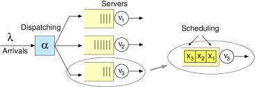
Dispatching problems arise in many contexts such as manufacturing sites, web server farms, super computing systems, and other parallel server systems. In a dispatching system jobs are assigned upon arrival to one of the several queues as illustrated in Fig. 1. Such systems involve two decisions: (i) dispatching policy chooses the server, and (ii) scheduling discipline the order in which the jobs are served. The dispatching decisions are irrevocable, i.e., it is not possible to move a job to another queue afterwards. In the literature, the dispatching problems and their solutions differ with respect to (i) optimization objective, (ii) available information, and (iii) scheduling discipline used in the servers.
Although the literature has generally addressed the mean sojourn time (i.e., response time) as the optimization objective, also other performance metrics can be relevant. One such metric is the slowdown111Yang and de Veciana refer to the slowdown as the bit-transmission delay (BTD) [30]. of a job, defined as the ratio of the sojourn time and the processing time (service requirement) [17, 9, 1]. The slowdown criterion combines efficiency and fairness and stems from the idea that longer jobs can tolerate longer sojourn time. The optimal scheduling discipline in this respect for a single server queue and a fixed number of jobs is the so-called shortest-processing-time-product222Wierman et al. refer to SPTP as the RS policy, a product of the remaining size and the original size [28]. (SPTP) discipline [30], where the index of a job is the product of the initial and remaining service requirements and the job with the smallest index is served first. With aid of Gittins index, we show that SPTP minimizes the mean slowdown in single server queues also in the dynamic case of Poisson arrivals, i.e., it is the optimal discipline for an M/G/1 queue with respect to the slowdown.
Then we derive value functions with respect to arbitrary job specific holding costs for an M/G/1 with the first-in-first-out (FIFO), the last-in-first-out (LIFO), the shortest-processing-time (SPT), the shortest-remaining-processing-time (SRPT) and SPTP scheduling disciplines, where the last three are size-aware. A value function essentially characterizes the queue state in terms of the expected costs in infinite time horizon for a fixed scheduling discipline. In this respect, our work generalizes the results of [19] to arbitrary job specific holding cost rates, and includes also the analysis of the slowdown specific SPTP scheduling discipline.
Finally, we apply the derived value functions to the dispatching problem so as to minimize the mean slowdown when the scheduling disciplines in each queue are fixed. We assume that the dispatcher is fully aware of the state of the system, i.e., of the tasks in each queue and their remaining service requirements. By starting with an arbitrary state-independent policy, we carry out the first-policy-iteration (FPI) step of the Markov decision processes (MDP) and obtain efficient state-dependent dispatching policies.
The rest of the paper is organized as follows. In Section II, we consider a single M/G/1 queue with respect to slowdown criterion, and prove the optimality of SPTP. In Section III, we derive the size-aware value functions with respect to arbitrary job specific holding cost rates for FIFO, LIFO and SPTP (SPT and SRPT are given in the Appendix). The single queue scheduling related results are utilized in Section IV to derive efficient dispatching policies, which are then evaluated in Section V. Section VI concludes the paper.
I-A Related Work
FIFO is perhaps the most common scheduling discipline due to its nature and ease of implementation. Other common disciplines are LIFO, SPT and SRPT. As for the objective, minimization of the mean sojourn time has been a popular choice. Indeed, SPT and SRPT, respectively, are the optimal non-preemptive and preemptive schedules with this respect [25]. For a recent survey on fairness and other scheduling objectives in a single server queue we refer to [27].
In the context of dispatching problems, FIFO has been studied extensively in the literature since the early work by Winston [29], Ephremides et al. [8], and others. Often the number of tasks per server is assumed to be known, cf., e.g., join-the-shortest-queue (JSQ) dispatching policy [29]. Even though FIFO queues have received the most of the attention, also other scheduling disciplines have been studied. For example, Gupta et. al consider JSQ with processor-sharing (PS) scheduling discipline in [12].
Only a few optimality results are known for the dispatching problems. Assuming exponentially distributed interarrival times and job sizes, [29] shows that JSQ with FIFO minimizes the mean waiting time when the number in each queue is available. Also [8] argues for the optimality of JSQ/FIFO when the number in each queue is available, while the Round-Robin (RR), followed by FIFO, is shown to be the optimal policy when it is only known that the queues were initially in the same state. [24] proves that RR/FIFO is optimal with the absence of queue length information if the job sizes have a non-decreasing hazard function. The RR results were later generalized in [23]. Whitt [26], on the other hand, provides several counterexamples where JSQ/FIFO policy fails. Crovella et al.[6] and Harchol-Balter et al. [14] assume that the dispatcher is aware of the size of a new job, but not of the state of the FIFO queues, and propose policies based on job size intervals (e.g., short jobs to one queue, and the rest to another). Feng et al. [10] later showed that such a policy is the optimal size-aware state-independent dispatching policy for homogeneous servers.
Also the MDP framework lends itself to dispatching problems. Krishnan [22] has utilized it in the context of parallel M/M/s-FIFO servers so as to minimize the mean sojourn time, similarly as Aalto and Virtamo [3] for the traditional M/M/1 queue. Recently, FIFO, LIFO, SPT and SRPT queues were analyzed in [19] with a general service time distribution. Similarly, PS is considered in [21, 20]. The key idea with the above work is to start by an arbitrary state-independent policy, and then carry out FPI step utilizing the value functions (relative values of states).
II M/G/1 Queue and Slowdown
In this section we consider a single M/G/1 queue with arrival rate . The service requirements are i.i.d. random variables with a general distribution.
We define the slowdown of a job as a ratio of the sojourn time to the service requirement ,
where one is generally interested in its mean value . Also other similar definitions exist. In the context of distributed computing, Harchol-Balter defines the slowdown as the “wall-time” divided by the CPU-time in [15]. Another common convention is to consider the ratio of the waiting time to the processing time (see, e.g., [13]), which is a well-defined quantity for non-preemptive systems. These different definitions, however, are essentially the same.
For non-preemptive work conserving policies, the sojourn time in queue comprises the initial waiting time and the consequent processing time . Thus, the mean slowdown is
Waiting time with FIFO is independent of the job size , and with aid of Pollaczek-Khinchin formula one obtains [13],
| (1) |
which underlines the fact that the mean slowdown may be infinite for a stable queue as for many common job size distributions, e.g., for an exponential distribution.
The mean slowdown in an M/G/1 queue with preemptive LIFO and PS disciplines is a constant for all job sizes,
| (2) |
Corollary 1
FIFO is a better scheduling discipline than LIFO in an M/G/1 queue with respect to slowdown iff
| (3) |
II-A Shortest-Processing-Time-Product (SPTP)
In [30], Yang and de Veciana introduced the shortest-processing-time-product (SPTP) scheduling discipline, which will serve the job such that
where and denote, respectively, the initial and remaining service requirement of job . Yang and de Veciana were able to show that SPTP is optimal with respect to the mean slowdown in a transient system where all jobs are available at time 0 and no new jobs arrive thereafter (i.e., a myopic approach). SPTP can be seen as the counterpart of the SRPT333Note that defining an index policy with indices , and gives SRPT, SPT and SPTP, respectively, where corresponds to the geometric mean of and . when instead of minimizing the mean sojourn time, one is interested in minimizing the mean slowdown.
We argue below that SPTP is the optimal scheduling discipline also in the corresponding dynamic system with Poisson arrivals. That is, we show that SPTP is optimal with respect to the slowdown in the M/G/1 queue. Our proof is based on the Gittins index approach.
II-B Gittins Index
Consider an M/G/1 queue with multiple job classes , . Let denote the class- arrival rate, and the probability that an arriving job belongs to class . In addition, let denote the generic service time related to class . The total load is denoted by . We assume that . The Gittins index [11, 2] for a class- job with attained service is defined by
where is the holding cost rate related to class . Note that, in addition to the attained service , the Gittins index is based on the (class-specific) distribution of the service time, but not on the service time itself. The Gittins index policy will serve the job such that
where refers to the class and to the attained service of job . Let denote the sojourn time of a class- job. We recall the following optimality result proved by Gittins [11, Theorem 3.28].
Theorem 1
Consider an multi-class queue. The Gittins index policy minimizes the mean holding costs,
among the non-anticipating scheduling policies.
The non-anticipating policies are only aware of the attained service times of each job and the service time distributions (but not on the actual service times). So, in general, non-anticipating policies do not know the remaining service times implying that, e.g., SPTP does not belong to non-anticipating disciplines. However, there is one exception: If the service times are deterministic, , then the remaining service times are available for the non-anticipating policies (with probability 1). In such a case, all policies are non-anticipating.
II-C Optimality of SPTP
Consider now an M/G/1 queue with a single class and load . Let and denote, respectively, the generic service and sojourn times of a job. In addition, let denote the conditional mean sojourn time of a job with service time ,
Assume first that the support of the service time distribution is finite. In other words, there are such that . The following result is an immediate consequence of Theorem 1 as soon as we associate class with the jobs with the same service time requirement . Note that the Gittins index is now clearly given by
with the optimal equal to .
Corollary 2
Consider an queue for which the support of the service time distribution is finite. Among all scheduling policies, the mean holding costs,
are minimized by the policy that will serve job such that
where and denote the class and the remaining service requirement of job .
In particular, if we choose , we see that the mean slowdown is minimized by SPTP:
Corollary 3
Consider an queue for which the support of the service time distribution is finite. SPTP minimizes the mean slowdown among all scheduling policies.
Since any service time distribution can be approximated with an arbitrary precision by discrete service time distributions, we expect that the above result holds also for general service time distributions. Note also that the choice , for all , results in the well-known optimality result of SRPT with respect to the mean sojourn time.
III Value Functions for M/G/1
In this section we analyze a single M/G/1 queue in isolation with FIFO, LIFO, and SPTP scheduling disciplines and derive expressions for the size-aware value functions with respect to arbitrary job specific holding costs. The corresponding results for SPT and SRPT are also given in the Appendix. As special cases, one trivially obtains the value functions with respect to the mean sojourn time and the mean slowdown. Thus, these results generalize the corresponding results in [19], where the size-aware value functions with respect to sojourn time are given (except for SPTP).
Holding cost model
Consider an M/G/1 queue with an arbitrary but fixed work conserving scheduling discipline and load . Each existing task incurs costs at some task specific holding cost rate denoted by for job . Assume that are i.i.d. random variables, . However, may depend on the corresponding service requirement . Both the service requirement and the holding cost become known upon arrival.
The cumulative cost during for an initial state is
where denotes the set of tasks present in the system at time . Similarly, the long-term mean cost rate is
which for an ergodic Markovian system reads
The value function is defined as the expected deviation from the mean cost rate in infinite time-horizon,
A value function characterizes how expensive it is to start from each state. In our setting, it enables one to compute the expected cost of admitting a job with size and holding cost rate to a queue, which afterwards behaves as an M/G/1 queue with the given scheduling discipline:
| (4) |
where denotes the state resulting from adding a new job in state . In Section IV we will carry out the FPI step in the context of dispatching problem, for which a corresponding value function is a prerequisite.
Size dependent holding cost
In general, the holding cost rate can be arbitrary, e.g., a class-specific i.i.d. random variable. However, in two important special cases, mean sojourn time and mean slowdown, it depends solely on the service requirement , :
| mean sojourn time: | ||||
| mean slowdown: |
In equilibrium, the average cost per job is . Using Little’s result, we have for the mean cost rate,
where denotes the mean number in the system.
III-A M/G/1-FIFO Queue
Next we derive the size-aware value function for an M/G/1-FIFO queue with respect to arbitrary job specific holding costs. To this end, let denote the remaining service requirements (measured in time) and the corresponding holding cost rates at state . The total rate at which costs are accrued at given state is thus the sum . Job is currently receiving service and job is the latest arrival. The total backlog is denoted by ,
Proposition 1
For the size-aware relative value in an M/G/1-FIFO queue with respect to arbitrary job specific holding costs it holds that
| (5) |
where is the mean holding cost rate for all later jobs.
Proof:
We compare two systems with the same arrival patterns, System 1 initially in state and System 2 initially empty. The two systems behave equivalently after System 1 becomes empty. The cost incurred by the current jobs, present only in System 1, is already fixed as
The later arriving jobs encounter a longer waiting time in System 1. The key observation here is that these jobs experience an additional delay of in System 1 when compared to System 2, as is illustrated in Fig. 2. Otherwise the sojourn times are equal. On average (mini) busy periods occur before System 1 becomes empty. These busy periods are independent and on average jobs are served during each of them. The average additional waiting time is . Therefore, the later arriving jobs incur on average
higher holding cost in System 1 than in System 2. Total cost difference is , which completes the proof. ∎

Corollary 4
The mean cost in terms of sojourn time due to accepting a job with size to a size-aware M/G/1-FIFO queue initially at state is
Corollary 5
The mean cost in terms of slowdown due to accepting a job with size to a size-aware M/G/1-FIFO queue initially at state is
| (6) |
III-B M/G/1-LIFO Queue
Next we derive the size-aware value function for the LIFO scheduling discipline. To this end, let us denote the state of the system with jobs by a vector , where denotes the remaining service requirement (measured in time) and the holding cost rate of job . Job is the latest arrival and currently receiving service (if any), i.e., without new arrivals the jobs are processed in the natural order: .
Proposition 2
For the size-aware relative value in a preemptive M/G/1-LIFO queue with respect to arbitrary job specific holding cost it holds that
| (7) |
Proof:
We compare System 1 initially in state and System 2 initially empty. The current state bears no meaning for the future arrivals with preemptive LIFO, and thus the difference in the expected costs is equal to the cost the current jobs in System 1 incur:
where denotes the remaining sojourn time of job [19],
which completes the proof. ∎
For the mean sojourn time, the holding cost rate is constant and a sufficient state description is .
Corollary 6
The cost in terms of sojourn time due to accepting a job with size to a size-aware preemptive M/G/1-LIFO queue at state is
For the slowdown, the initial service requirements define the holding costs and a sufficient state description is , where and denote the remaining and initial service requirement of job , so that the holding cost of job is :
Corollary 7
The cost in terms of slowdown due to accepting a job with size to a size-aware preemptive M/G/1-LIFO queue at state is
| (8) |
III-C M/G/1-SPTP Queue
Next we derive the corresponding size-aware value function for the SPTP scheduling discipline. The state description for SPTP is , where, without loss of generality, we assume a decreasing priority order, i.e., the job (if any) is currently receiving service. Then, denotes the amount of work with a higher priority than ,
Let , and denote the arrival rate, mean job size and offered load due to jobs shorter than ,
| (9) |
where denotes the job size pdf.
Lemma 1
The mean remaining sojourn time of a -job in an M/G/1-SPTP queue initially in state is given by
| (10) |
Proof:
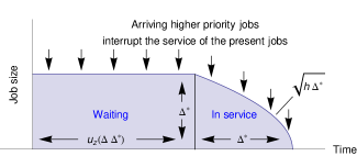
Let denote the -job, whose remaining sojourn time depends on the initial and later arriving higher priority work. We can assume that the latter are served immediately according to LIFO, thus triggering mini busy periods. Let denote the remaining service time of job at (virtual) time , where we have omitted these mini busy periods from the time axis. During , job is waiting and , but as the service begins linearly. The later arriving higher priority jobs shorter than constitute an inhomogeneous Poisson process with rate , as illustrated in Fig. 3. The mean duration of a mini busy period is (cf. the mean busy period in M/G/1),
The mean waiting time before job receives service for the first time is , which gives the first term in (10).

Even though SPTP explicitly tries to minimize the mean slowdown, we derive next a general expression for the value function with arbitrary job specific holding costs:
Proposition 3
For the size-aware relative value in an M/G/1-SPTP queue with respect to arbitrary job specific holding costs it holds that
| (11) |
where and
Proof:
The relative value comprises the mean holding cost accrued by the current tasks in state ,
and the difference in costs accrued by the later arriving jobs, , . The first summation over gives , i.e., it follows from multiplying (10) with the job specific holding cost and adding over all .
The latter integral corresponds to where the accrued costs are conditioned on the size of an arriving job. The corresponding arrival rate is . The mean difference in sojourn time experienced by an arriving job with size is accrued during the initial waiting time – once a job enters the service for the first time its mean remaining sojourn time is the same in both systems. The initial waiting time is a function of higher priority workload upon arrival, denoted by for an initial state at arrival time . In particular, the mean (initial) waiting time is simply , which gives
Next we refer to Fig. 4 and observe that in the integrand corresponds to area A. This area consists of one triangle, followed by rectangles, and similar sequences starting with a triangle for , each followed by rectangles. The are random variables corresponding to the number of mini busy periods during the service time of a particular triangle. The first triangle corresponds to the initially higher priority workload , and the latter to the jobs with initially lower priority, i.e., to jobs with . At some point in time, the remaining service requirement of such a job decreases to and its priority index drops below . For a sequence starting with a -triangle, the number of mini busy periods (rectangles) obeys Poisson distribution with mean . The height of a rectangle is uniformly distributed in having the mean (property of Poisson process), while the width corresponds to the duration of a busy period in a work conserving M/G/1 queue having the mean . Thus, the mean total area is
Therefore,
where factor in the numerator corresponds to the mean holding cost of an -job. For each interval , and
and integration in parts completes the proof. ∎
Recall that with respect to the mean sojourn time, and , while for the slowdown criterion, and . Hence, (11) allows one to compute the mean cost due to accepting a given job in terms of sojourn time or slowdown. We omit the explicit expression for for brevity.
The corresponding value functions for SPT and SRPT are derived in the Appendix. The numerical evaluation of the value function for SPTP, SPT and SRPT is not as unattractive as it first may seem. Basically one needs to be able to compute integrals of form
where and depending on the discipline. Thus, e.g., a suitable interpolation of the and enables on-line computation of the value function.
IV Dispatching Problem
Next we utilize the results of Section III in the dispatching problem with parallel servers and focus solely on minimizing the mean slowdown. The dispatching system illustrated in Fig. 1 comprises servers with service rates . Jobs arrive according to a Poisson process with rate and their service requirements are i.i.d. random variables with a general distribution. The jobs are served according to a given scheduling discipline (e.g., FIFO) in each server.
The slowdown for an isolated queue was defined as the sojourn time divided by the service requirement [17] (both measured in time), . However, as we consider heterogeneous servers with rates , the service requirement of size job (measured, e.g., in bytes) is no longer unambiguous but a server specific quantity,
Therefore, for a dispatching system we compare the sojourn time to the hypothetical service time if all capacity could be assigned to process a given job [7],
The relationship between the queue specific slowdown and the system wide slowdown is .
IV-A Random Dispatching Policies
The so-called Bernoulli splitting assigning jobs independently in random using probability distribution offers a good state-independent basic dispatching policy. Due to Poisson arrivals, each queue also receives jobs according to a Poisson process with rate .
Definition 1 (RND-)
The RND- dispatching policy balances the load equally by setting .
As an example, the mean slowdown in a preemptive LIFO or PS queue with RND- policy is,
where the denominator corresponds to the excess capacity. Thus, with RND- and LIFO queues, the slowdown criterion is times higher when servers are used instead of a single fast one irrespectively of the service rate distribution .
For identical servers, , the RND- dispatching policy reduces to RND-U:
Definition 2 (RND-U)
The RND-U dispatching policy assigns jobs randomly in uniform using .
RND-U is obviously the optimal random policy in case of identical servers.
In general, the optimal splitting probabilities depend on the service time distribution and the scheduling discipline. For the preemptive LIFO (and PS) server systems the mean slowdown with a random dispatching policy is given by
where is a constant that can be neglected when optimizing the .
Definition 3 (RND-opt)
The optimal random dispatching policy for LIFO/PS queues, referred to as RND-opt, splits the incoming tasks using the probability distribution,
The result is easy to show with the aid of Lagrange multipliers. We note that when some servers are too slow, the above gives infeasible values for some , in case of which one simply excludes the slowest server from the solution and re-computes a new probability distribution. This is repeated until a feasible solution is found. A more explicit formulation is given in [5, 18]. RND-opt is insensitive to the job size distribution and optimal only for LIFO and PS.
Pollaczek-Khinchin mean value formula enables one to analyze FIFO queues and, e.g., to write an expression for the mean slowdown with RND-. Also the optimal splitting probabilities can be computed numerically for an arbitrary job size distribution. According to (1), the mean slowdown in each queue depends on the mean waiting time and , where the latter is assumed to exist and to be finite. Hence, the optimal probability distribution with respect to slowdown is the same as with the mean sojourn time.
Similarly, the mean sojourn time in SPT and SRPT queues is known which allows a numerical optimization of the splitting probabilities. For simplicity, we consider only RND- and RND-opt in this paper as compact closed form expressions for the are only available for these.
IV-B SITA-E Dispatching Policy
With FIFO queues, a state-independent dispatching policy known as the size-interval-task-assignment (SITA) has proven to be efficient especially with heavy-tailed job size distributions [6, 14, 4]. The motivation behind SITA is to segregate the long jobs from the short ones. Reality, however, is more complicated and segregating the jobs categorically can also give suboptimal results [16]. Here we assume and a continuous job size distribution with pdf .
Definition 4 (SITA)
A SITA policy is defined by disjoint job size intervals , , , , and assigns a job with size to server iff .
Without loss of generality, one can assume that and . Note that in contrast to random policies, SITA assumes that the dispatcher is aware of the size of the new job. In this paper, we limit ourselves to SITA-E, where E stands for equal load. That is, the size intervals are chosen in such a way that the load is balanced between the servers.
Definition 5 (SITA-E)
With SITA-E dispatching policy the thresholds are defined in such a way that
Thus, similarly as RND-, also the SITA-E policy is insensitive to the arrival rate .
IV-C Improved Dispatching Policies
The important property the above state-independent dispatching policies have is that the arrival process to each queue is a Poisson process. Consequently, the value functions derived earlier allow us to quantify the value function of the whole system. With a slight abuse of notation,
where denotes the relative value of queue in state , and the state of the whole system.
Policy Improvement by Role Switching
One interesting opportunity to utilize the relative values is to switch the roles of two queues [19]. Namely, with an arbitrary state-independent policy one can switch the input processes of any two identical servers at any moment, and effectively end up to a new state of the same system. Despite its limitation (identical servers), switching is an interesting policy improvement method that requires little additional computation. The switch should only be carried out when the new state has lower expected future costs, i.e. when for some , the rates are equal, , and
Carrying out this operation whenever a new job has arrived to the system reduces the state-space by removing such states for which a better alternative to continue exists. Formally, let denote the set of feasible permutations of the queues’ roles, where the input processes between identical servers are switched. Then, the optimal state-space reduction, implicitly defining a new policy, is given by
To elaborate this, consider a RND-/LIFO system. In this case, (7) implies that switching the roles of any two identical queues makes no difference to the relative value.
In contrast, with FIFO discipline the interesting quantity from (5) for two identical servers and is identified to be
Switching the input processes between queues and leads to a state with a lower relative value if . Again, with RND- the factor is a constant for any two identical servers and switching provides no gain. However, with SITA-E, even though the denominator is a constant, the numerator is not. Let denote a job size in queue . Then , and therefore . Moreover, , yielding
Consequently, with the SITA-E with switch policy, the optimal permutation, after inserting a new job to a queue, is the one with increasing backlogs for identical servers:
Definition 6 (SITA-Es)
SITA-E with switch dispatching policy behaves similarly as SITA-E with a distinction that after each task assignment the queues are permutated in such a way that for all identical servers and .
Policy Improvement by FPI
The first-policy-iteration (FPI) is a general method of the MDP framework to improve any given policy. We apply it to the dispatching problem [19]. Suppose that the scheduling discipline in each queue is fixed and that a state-independent basic dispatching policy would assign a new job to some queue. Given the relative values and the expected cost associated with accepting the job to each queue, we can carry out FPI: we deviate from the default action if the expected cost is smaller with some other action, thereby decreasing the expected cumulative costs in infinite time horizon.
Let denote the arrival rate to queue according to the basic dispatching policy, and the corresponding job size. With a state-independent policy, accepting a job to queue does not affect the future behavior of the other queues. Thus, the cost of assigning a job with size to queue is
where is the mean admittance cost of a job with size (measured, e.g., in bytes) to queue , where its service requirement (measured in time) would be . For slowdown, we have an elementary relation
For FIFO queues, (6) gives
For preemptive LIFO queues, (8) similarly gives
where denotes the number of jobs in queue and the initial service requirement (in time) of job in queue . According to the FPI principle, one simply chooses the queue with the smallest (expected) cost,
| (12) |
We refer to these improved dispatching policies simply as the FPI- policy, where denotes the basic dispatching policy, e.g., RND-opt or RND-, where for brevity reasons the RND prefix is often omitted. Note that the factor in both expressions is a common constant for all queues.
| RND- | state-independent random policy with load balancing |
|---|---|
| RND-opt | state-independent random policy minimizing the mean slowdown (assumes LIFO/PS) |
| SITA-E | state-independent size-interval-task-assignment with equal loads (optionally, with switch) |
| Round-Robin | assigns arriving tasks sequentially to servers [8] |
| LWL- | least-work-left, assigns a job to server with the least amount unfinished work upon arrival |
| LWL+ | same as LWL- but based on the unfinished work (in time) including the new job [19] |
| JSQ | join-the-shortest-queue, i.e., the one with the least number of jobs [29] |
| Myopic | minimize the mean slowdown on condition that no further jobs arrive |
| FPI | first policy iteration on the state-independent RND-, RND-opt and SITA-E policies |
In a symmetric case of identical servers and the RND-U basic policy, a corresponding FPI-based policy reduces to a well-known dispatching policy, i.e., with FIFO queues, FPI yields LWL, and with LIFO, the Myopic policy (see Table I). Moreover, given additionally a constant job size, then in case of LIFO queues one ends up with the JSQ policy. In general, for constant job sizes the slowdown objective reduces to the minimization of the mean sojourn time.
|
|
|
|---|---|
| (a) Two identical servers | (b) Three heterogeneous servers |
V Numerical Examples
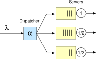
Let us next evaluate by means of numerical simulations the improved dispatching policies derived in Section IV. To this end, we have chosen to consider two elementary server systems that are illustrated in Fig 5:
-
(a)
Two identical servers with rates ,
-
(b)
Three heterogeneous servers with rates and .
Thus, the total service rate in both systems is equal to . We compare the mean slowdown performance of the FPI policies against several well-known heuristic dispatching policies, including the state-independent policies RND-opt, RND- and SITA-E. The somewhat more sophisticated least-work-left (LWL) policies choose the queue with the least amount of unfinished work (backlog). The difference between the LWL policies is that LWL- considers the situation without the new job, and LWL+ afterwards. With identical servers the LWL policies are equivalent. JSQ chooses the queue with the least number of jobs. With the LWL and JSQ, the ties are broken in favor of a faster server. The Myopic policy assumes in a greedy fashion that no further jobs arrive and chooses the queue which minimizes the immediate cost the known jobs accrue. All policies are listed in Table I.
In many real-life settings, the job sizes have been found to exhibit a heavy-tailed behavior, (cf., e.g., file sizes in the Internet). Thus, in most examples we assume a bounded Pareto distribution with pdf
| (13) |
where so that . This job size distribution is particularly suitable for SITA-E.
V-A FIFO
First we assume that servers operate under the FIFO scheduling discipline and job sizes obey the bounded Pareto distribution (13). With FIFO, the departure time gets fixed at dispatching and the Myopic policy corresponds to selfish users choosing the queue that guarantees the shortest sojourn time, i.e., LWL+. Similarly, LWL- is equivalent to an M/G/ system with a single shared queue.
Two identical servers
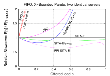
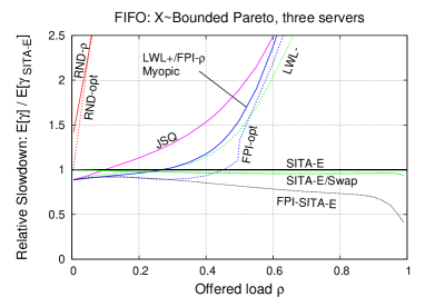
Fig. 6 (left) depicts the results with two identical servers with rates . The -axis corresponds to the offered load and the -axis to the relative mean slowdown, , i.e., the comparison is against SITA-E. We find that the policies appear to fall in one of the three groups with respect to slowdown: SITA policies form the best group, other queue state-dependent policies the next, and RND-U and Round-Robin have the worst performance. Especially, FPI-SITA-E outperforms the other policies by a significant margin, including the other SITA policies. Note also that when is small, the sensible state-dependent policies utilize idle servers better than, e.g., SITA-E.
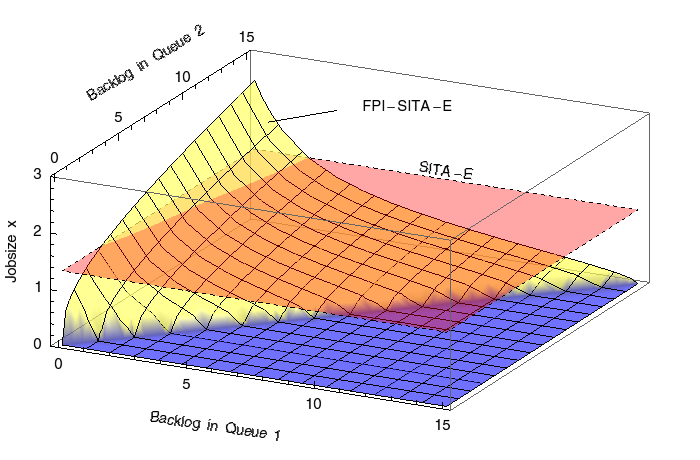
Fig. 7 illustrates SITA-E and FPI-SITA-E in the same setting at an offered load of . The - and -axes correspond to the backlog in Queue 1 and Queue 2, respectively, and the -axis to the maximum job size a given policy assigns to Queue 1. With SITA-E, this threshold is constant, while FPI-SITA-E changes the threshold dynamically. One observes that as a result of FPI, Queue 1 has become a “high-priority” queue where no jobs are accepted whenever Queue 1 has more unfinished work than Queue 2. Similarly, when Queue 2 has a long backlog, the threshold for assigning a job to Queue 1 becomes higher with FPI than with SITA-E.
Three heterogeneous servers
Consider next the asymmetric setting comprising one primary server with service rate and two secondary servers with rates . Fig. 6 (right) illustrates the results from a numerical simulation.
The state-independent random policies are much worse than the other policies. However, state-independent SITA-E again proves out to be better than the state-dependent policies JSQ, LWL-, LWL+, Myopic, FPI- and FPI-opt. The gain from switching the roles of the queues (SITA-E vs. SITA-Es) is smaller in this case due to the fact that we may only switch the roles of the two slower queues having the same service rate . As expected, the FPI-SITA-E policy yields a significantly lower mean slowdown than any other policy especially under a heavy load.
Based on the results, one can assume that the relative values obtained for the random policies simply do not capture the situation sufficiently well, while SITA-E is already a good dispatching policy, and FPI then leads to “adaptive” size intervals.
V-B Preemptive LIFO
Next we assume that the servers are bound to operate under LIFO, which, as mentioned, has a reasonably robust performance with respect to the mean slowdown. Job sizes are again assumed to obey the bounded Pareto distribution.
Two identical servers
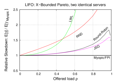
Fig. 8 (left) illustrates the performance with respect to the slowdown criterion for two identical servers. On -axis is again the offered load and -axis corresponds to the relative mean slowdown (here comparison is against the Myopic policy). One can identify three performance groups: RND and LWL form the worst performing group, then come Round-Robin and JSQ, and the Myopic and FPI-RND policy achieve the lowest mean slowdown.
Three heterogeneous servers
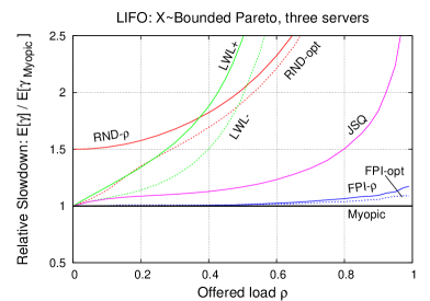
Fig. 8 (right) illustrates the simulation results in the asymmetric setting comprising one primary server with service rate and two secondary servers with rates . In this case, the Myopic approach is the optimal (among the candidates) while both FPI policies attain almost identical mean slowdown. Even though the value function for the Myopic policy is not available for us, one can estimate the relative values by means of simulation and carry out the policy improvement numerically. However, in this paper we do not pursue into this direction.
 |
 |
Server constellations
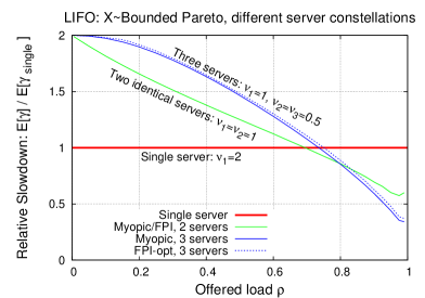
In Fig. 9 we compare the mean slowdown between different server constellations assuming the preemptive LIFO scheduling discipline. The -axis represents the relative performance when compared to the two server system. To no surprise, when the load is small or moderate, a single server system achieves the lowest mean slowdown. However, as the load increases more, first the two server system becomes optimal, and then eventually the three server system takes the lead. This is due to the fact that at higher load levels, the correct dispatching decisions allow one to serve more expensive jobs faster. One interesting research question indeed is that given a total capacity budget, what is the optimal server constellation so as to minimize the mean slowdown.
V-C SPTP
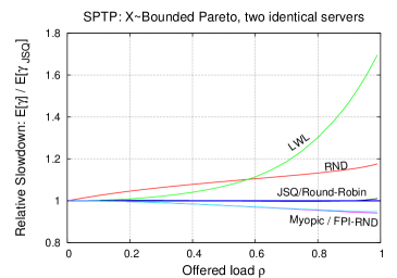
Finally, let us consider the SPTP scheduling discipline that is the natural choice when minimizing the mean slowdown (see Section II). The job sizes are again assumed to obey the bounded Pareto distribution. Fig. 10 (left) illustrates the slowdown performance with the two identical servers. Interestingly, LWL becomes even weaker than RND-U as the offered load increases. Myopic and FPI-RND achieve the lowest mean slowdown.
In the case of three heterogeneous servers, the situation is again more challenging and the numerical results are depicted in Fig. 10 (right). At low levels of load, RND-opt is a surprisingly good choice, suggesting that SPTP manages to locally “correct” the occasional suboptimal decisions. When the load increases, the LWL policies become weak again. The Myopic policy shows a robust and good performance at all levels of offered load. However, the FPI policies, and FPI-opt in particular, achieve the lowest mean slowdown which is significantly better than with any other policy when .
V-D Comparison of scheduling disciplines
 |
 |
| (a) | (b) |
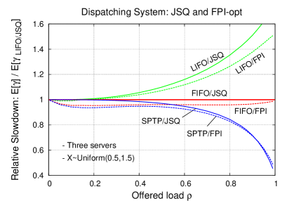
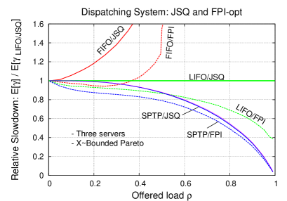
So far we have fixed a scheduling discipline and evaluated different dispatching policies. Here we give a brief comparison of different scheduling disciplines with respect to the slowdown metric. Job sizes obey either (a) uniform distribution, , or (b) the bounded Pareto distribution, both having the same mean, .
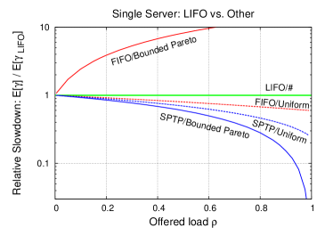
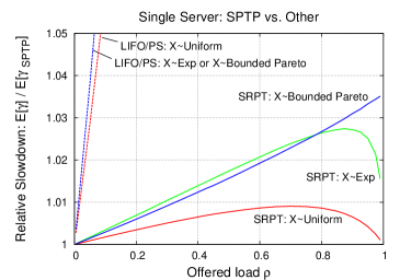
First we consider a single server queue. Fig. 11 (left) depicts a comparison against LIFO with the same job size distribution on the logarithmic scale. In accordance with (3), FIFO is better than LIFO with uniform job size distribution, and with the bounded Pareto distribution the situation is the opposite. SPTP is clearly the best in both cases. In Fig. 11 (right), the reference level is the mean slowdown with SPTP. Here we have included also SRPT, which turns out to be only marginally better than SRPT, as observed also in [28]. LIFO and PS are significantly worse.
Fig. 12 illustrates the relative performance between different scheduling disciplines and dispatching policies in the heterogeneous three server dispatching system. SRPT is not included as its performance is very similar to SPTP. The reference level is the mean slowdown a JSQ/FIFO (left) and JSQ/LIFO (right) achieve. FPI manages to outperform the corresponding JSQ policy in all cases. Especially with the bounded Pareto distributed job sizes, FPI/LIFO performs rather well when compared to JSQ/LIFO. SPTP is clearly superior scheduling discipline in both cases, as expected.
In general, the scheduling discipline seems to have a stronger influence to the performance than the dispatching policy.
VI Conclusions
This work generalizes the earlier results of the size-aware value functions with respect to the sojourn time for M/G/1 queues with FIFO, LIFO, SPT and SRPT disciplines to a general job specific holding cost. Additionally, we have considered the SPTP queueing discipline, the optimality of which with Poisson arrivals was also established. As an important special case, one obtains the slowdown criterion, where the holding cost is inversely proportional to the job’s (original) size. These results were then utilized in developing robust policies for dispatching systems. In particular, the value functions enable the policy improvement step for an arbitrary state-independent dispatching policy such as Bernoulli-splitting. The derived dispatching policies were also shown to perform well by means of numerical simulations. In particular, the highest improvements were often obtained in a more challenging heterogeneous setting with unequal service rates. Also the SPTP scheduling discipline outperformed the other by a clear margin in the examples, except the SRPT discipline, which appears to offer a rather similar performance in terms of slowdown and sojourn time.
References
- [1] S. Aalto, U. Ayesta, S. Borst, V. Misra, and R. Núñez-Queija. Beyond processor sharing. SIGMETRICS Perform. Eval. Rev., 34:36–43, 2007.
- [2] S. Aalto, U. Ayesta, and R. Righter. On the Gittins index in the M/G/1 queue. Queueing Systems, 63(1-4):437–458, 2009.
- [3] S. Aalto and J. Virtamo. Basic packet routing problem. In NTS-13, Trondheim, Norway, Aug. 1996.
- [4] E. Bachmat and H. Sarfati. Analysis of SITA policies. Performance Evaluation, 67(2):102–120, 2010.
- [5] C. E. Bell and J. Shaler Stidham. Individual versus social optimization in the allocation of customers to alternative servers. Management Science, 29(7):831–839, July 1983.
- [6] M. E. Crovella, M. Harchol-Balter, and C. D. Murta. Task assignment in a distributed system: Improving performance by unbalancing load. In ACM SIGMETRICS, pages 268–269, June 1998.
- [7] A. Downey. A parallel workload model and its implications for processor allocation. In IEEE HPDC’97, pages 112–123, Aug. 1997.
- [8] A. Ephremides, P. Varaiya, and J. Walrand. A simple dynamic routing problem. IEEE Transactions on Automatic Control, 25(4):690–693, Aug. 1980.
- [9] H. Feng and V. Misra. Mixed scheduling disciplines for network flows. SIGMETRICS Perform. Eval. Rev., 31:36–39, Sept. 2003.
- [10] H. Feng, V. Misra, and D. Rubenstein. Optimal state-free, size-aware dispatching for heterogeneous M/G/-type systems. Perform. Eval., 62(1-4), 2005.
- [11] J. Gittins. Multi-armed Bandit Allocation Indices. Wiley, 1989.
- [12] V. Gupta, M. Harchol-Balter, K. Sigman, and W. Whitt. Analysis of join-the-shortest-queue routing for web server farms. Performance Evaluation, 64(9-12):1062–1081, Oct. 2007.
- [13] M. Harchol-Balter. Task assignment with unknown duration. J. ACM, 49(2):260–288, Mar. 2002.
- [14] M. Harchol-Balter, M. E. Crovella, and C. D. Murta. On choosing a task assignment policy for a distributed server system. Journal of Parallel and Distributed Computing, 59:204–228, 1999.
- [15] M. Harchol-Balter and A. B. Downey. Exploiting process lifetime distributions for dynamic load balancing. ACM Transactions on Computer Systems, 15(3):253–285, Aug. 1997.
- [16] M. Harchol-Balter, A. Scheller-Wolf, and A. R. Young. Surprising results on task assignment in server farms with high-variability workloads. In ACM SIGMETRICS, pages 287–298, 2009.
- [17] M. Harchol-Balter, K. Sigman, and A. Wierman. Asymptotic convergence of scheduling policies with respect to slowdown. Perform. Eval., 49(1-4):241–256, Sept. 2002.
- [18] M. Haviv and T. Roughgarden. The price of anarchy in an exponential multi-server. Oper. Res. Lett., 35(4):421–426, 2007.
- [19] E. Hyytiä, A. Penttinen, and S. Aalto. Size- and state-aware dispatching problem with queue-specific job sizes. European Journal of Operational Research, 217(2):357–370, Mar. 2012.
- [20] E. Hyytiä, A. Penttinen, S. Aalto, and J. Virtamo. Dispatching problem with fixed size jobs and processor sharing discipline. In ITC’23, SFO, USA, Sept. 2011.
- [21] E. Hyytiä, J. Virtamo, S. Aalto, and A. Penttinen. M/M/1-PS queue and size-aware task assignment. Performance Evaluation, 68(11):1136–1148, Nov. 2011.
- [22] K. R. Krishnan. Joining the right queue: a state-dependent decision rule. IEEE Transactions on Automatic Control, 35(1):104–108, Jan. 1990.
- [23] Z. Liu and R. Righter. Optimal load balancing on distributed homogeneous unreliable processors. Operations Research, 46(4):563–573, 1998.
- [24] Z. Liu and D. Towsley. Optimality of the round-robin routing policy. Journal of Applied Probability, 31(2):466–475, June 1994.
- [25] L. Schrage. A proof of the optimality of the shortest remaining processing time discipline. Operations Research, 16(3), 1968.
- [26] W. Whitt. Deciding which queue to join: Some counterexamples. Oper. Res., 34(1):55–62, 1986.
- [27] A. Wierman. Fairness and scheduling in single server queues. Surveys in Operations Research and Management Science, 16(1):39–48, 2011.
- [28] A. Wierman, M. Harchol-Balter, and T. Osogami. Nearly insensitive bounds on SMART scheduling. In ACM SIGMETRICS, pages 205–216, 2005.
- [29] W. Winston. Optimality of the shortest line discipline. Journal of Applied Probability, 14:181–189, 1977.
- [30] S. Yang and G. de Veciana. Size-based adaptive bandwidth allocation: optimizing the average QoS for elastic flows. In IEEE INFOCOM, 2002.
Appendix A Value Function for SPT and SRPT
Carrying out the similar steps as with SPTP, it is straightforward to derive value function also in the case of SPT and SRPT policies. Again, we let denote the pdf of the job size distribution and the offered load due to jobs shorter than according to (9). The backlog due to higher priority work in this case is , i.e., where the priority index for SPT is the initial service time , and for SRPT the remaining service time .
A-A M/G/1-SPT
We consider the non-preemptive SPT, which is the optimal non-preemptive schedule with respect to both the mean sojourn time and the mean slowdown. Thus, the remaining service time of a queueing job is equal to the initial service time. Therefore, a sufficient state description for a non-preemptive M/G/1-SPT queue with arbitrary holding costs is , where job (if any) is currently receiving service and jobs are waiting in the queue. Without lack of generality, we can assume that .
Proposition 4
For the size-aware value function with respect to arbitrary holding costs in an non-preemptive M/G/1-SPT queue it holds that,
| (14) |
where and the integration intervals are
Proof:
Similarly as with the SPTP, we compare two systems: System 1 initially in state and System 2 initially empty. The two systems behave identically once System 1 becomes empty for the first time. We can write , where is the cost the jobs initially present (only) in System 1 incur, and the difference in cost the later arriving customers incur between the two systems.
First, the remaining sojourn time of job in a non-preemptive M/G/1-SPT queue is
| (15) |
which holds for all jobs present only in System 1. Therefore, their contribution to the is
For the later arriving jobs, we condition the derivation on job sizes , which arrive at rate of . Let denote the mean additional sojourn time such jobs experience in System 1 when compared to System 2. Let so that we have an expression for
Instead of considering actual arrivals, we focus on a rate at which virtual costs are accrued in order to find . With aid of (15), one can deduce that the virtual cost rate is equal to
where denotes the amount of work at time that would be processed before an arriving size job when a system was initially in state . In particular, we can write
which gives
Let denote the number of jobs waiting in the queue with a remaining service time greater than .
Due to the non-preemptive discipline, the evolution of for consists of phases. Let . During the first phase jobs are served and the initial backlog size jobs see is . The second phase starts when job enters the server and cannot be preempted, thus creating an initial backlog for size jobs, etc.

Considering arrival sample paths, one can deduce that the difference corresponds to the white marked region in Fig. 13, which consists of statistically independent areas. The area of a phase starting with an initial backlog of from size customers’ point of view is given by
| (16) |
Defining
then gives
For example, when , all current jobs in System 1 have a higher priority constituting a single phase with , etc. Next define the integration intervals, , for , and . Substituting these into the above gives
which completes the proof. ∎
A-B M/G/1-SRPT
While SPT was optimal in the class of non-preemptive schedules, the SRPT discipline is the optimal preemptive schedule [25]. For SRPT, a sufficient state description is , where, without loss of generality, we again can assume that job is currently receiving service (if any) and . For the total higher priority workload we have .
Proposition 5
For the size-aware value function in an M/G/1-SRPT queue with arbitrary holding cost it holds that
| (17) |
where and
Proof:
Again, we consider System 1 initially in state and System 2 initially empty, and find expressions for and corresponding to the cost the jobs initially present (only) in System 1 incur, and the difference in cost the later arriving customers incur between the two systems.
In a M/G/1-SRPT queue at state , the mean remaining sojourn time of a job with a (remaining) size and an unfinished work ahead in the queue is given by [19]
| (18) |
which gives the expected cost the current jobs444Note that we assume the opposite order than [19]. present in System 1 incur,
For the later arriving jobs, we can again write
which describes the expected difference in the cumulative sojourn times between System 1 and System 2 for size jobs.

With SRPT also the jobs in System 1 initially longer than affect the result as eventually, one at a time, they decrease below the threshold and trigger a new higher priority workload present only in System 1 (see Fig. 14). Consequently, we have one phase starting with a backlog of , and then phases starting with a backlog of , where denotes the number of jobs longer than in state . In some sense, this is the same as with SPT, but the difference is the initial backlog size jobs see: with SPT it is instead of for later phases. Hence, each of these phases reduce to (16), which gives
As , and both and are (monotonic) step functions having jumps at , we proceed by integrating in parts. Defining
then gives
and recalling that then gives (17). ∎