The role of super-asymptotic giant branch ejecta in the abundance patterns of multiple populations in globular clusters

Abstract

Star formation from matter including the hot CNO processed ejecta of asymptotic giant branch (AGB) winds is regarded as a plausible scenario to account for the chemical composition of a stellar second generation (SG) in Globular Clusters (GCs). The chemical evolution models, based on this hypothesis, so far included only the yields available for the massive AGB stars, while the possible role of super–AGB ejecta was either extrapolated or not considered. In this work, we explore in detail the role of super–AGB ejecta on the formation of the SG abundance patterns using yields recently calculated by Ventura and D’Antona.

An application of the model to clusters showing extended Na–O anticorrelations, like NGC 2808, indicates that a SG formation history similar to that outlined in our previous work is required: formation of an Extreme population with very large helium content from the pure ejecta of super–AGB stars, followed by formation of an Intermediate population by dilution of massive AGB ejecta with pristine gas. The present models are able to account for the very O-poor Na-rich Extreme stars once deep-mixing is assumed in SG giants forming in a gas with helium abundance Y$>0.34$, which significantly reduces the atmospheric oxygen content, while preserving the sodium abundance. On the other hand, for clusters showing a mild O–Na anticorrelation, like M 4, the use of the new yields broadens the range of SG formation routes leading to abundance patterns consistent with observations. Specifically, our study shows that a model in which SG stars form only from super–AGB ejecta promptly diluted with pristine gas can reproduce the observed patterns. We briefly discuss the variety of (small) helium variations occurring in this model and its relevance for the horizontal branch morphology.

In some of these models, the duration of the SG formation episode can be as short as $\sim 10$ Myr; the formation time of the SG is therefore compatible with the survival of a cooling flow in the cluster core, previous to the explosion of the SG core collapse supernovae. We also explore models characterized by the formation of multiple populations in individual bursts, each lasting no longer than $\sim$10 Myr.

1 Introduction

The presence of multiple stellar populations, in all globular clusters (GCs) so far spectroscopically examined, is shown with convincing evidence in the recent analysis of Carretta et al. (2009a) of about two thousand stars in 19 GCs. Each cluster displays a sodium – oxygen anticorrelation (though the extension of the anticorrelation differ from cluster to cluster) due to the existence of a population of stars which are richer in sodium and poorer in oxygen than halo stars with the same metallicity. The Na–O anti–correlation is typical of GCs, whose constituent stars belong to two or more stellar populations differing in the abundances of the elements produced by the hot CNO cycle and by other proton–capture reactions on light nuclei. In fact, these chemical signatures are present also in turn–off stars and among the subgiants (e.g. Gratton et al., 2001; Briley et al., 2002, 2004), so they can not be due to “in situ” mixing in the stars, but must be due to some process of self–enrichment occurring at the first stages of the cluster life.

Photometric evidences for the presence of multiple populations are also numerous, and sometimes suggestive of star formation occurring in separate successive bursts. The photometric signatures of different populations can be ascribed in part to helium differences, inferred from the morphology of the horizontal branches (HB) (D’Antona et al., 2002; D’Antona & Caloi, 2004; Lee et al., 2005), or from the presence of multiple main sequences (MS), in $\omega$ Cen (Norris, 2004; Piotto et al., 2005) and NGC 2808 (D’Antona et al., 2005; Piotto et al., 2007). The strong link between the abundance anomalies (sodium rich and sodium poor groups) in the cluster M 4 (Marino et al., 2008) and their location on the HB is proven by Marino et al. (2011), who find that the blue HB stars of M 4 have high sodium, while the red HB stars have normal sodium. This supports the interpretation that there is a slight increase in the helium abundance of the “anomalous” stars (the sodium rich group) (D’Antona et al., 2002).

Two other important links between photometric and spectroscopic evidence have been recently given. The first one comes from the analysis of elemental abundances of two main sequence (MS) stars in NGC 2808 (Bragaglia et al., 2010) showing that the blue MS star only has “anomalous” sodium and aluminum. This supports the interpretation that the blue MS was formed from helium rich, CNO processed gas. The second link has been stressed most recently by Pasquini et al. (2011) who, directly comparing the He I 10 830 Å lines in the spectra of two NGC 2808 giants having different O and Na abundances, find direct evidence of a significant He line strength difference. From a detailed chromospheric modeling, they show that the difference in the spectra is consistent and most closely explained by an He abundance difference between the two stars of $\Delta$Y $\geq$0.17, consistent with the expected difference in abundance required by stellar models to account for the blue MS.

Based on these and on a large body of other complex evidences, the formation of globular clusters is now schematized as a two–step process, lasting no longer than $\sim$100 Myr, during which the nuclearly processed matter from a “first generation” (FG) of stars gives birth, in the cluster innermost regions, to a “second generation” (SG) of stars with the characteristic signature of a distribution of element abundances fully CNO–cycled.

Two main scenarios have been proposed to identify the matter constituting the SG stars: these could have formed either from the gaseous ejecta of massive asymptotic giant branch (AGB) stars (“AGB scenario”; Ventura et al., 2001; D’Antona & Caloi, 2004; Karakas et al., 2006) or from the ejecta of fast rotating massive stars (“FRMS scenario”; Prantzos & Charbonnel, 2006; Meynet et al., 2006; Decressin et al., 2007). These studies investigated whether the observed abundance patterns found in GCs can be accounted for by models. Problems are present in both scenarios (see, e.g., Renzini, 2008, for a critical review).

In order to go from a “scenario” to a “model”, the SG formation must be investigated quantitatively, and must rely as far as possible on computed models. From this point of view, very few are the “models” available in the literature, in spite of the large number of works recently published on this subject. In particular, the O–Na anticorrelation is a signature present in all cluster, but the cluster-to-cluster differences are very large: some clusters (the most massive ones) show very extended anticorrelations, down to values of [O/Fe], more than 1 dex smaller than the values of the FG stars, other clusters show a “mild” anticorrelation, in which [O/Fe] is reduced by $\sim$0.2–0.3 dex. In addition, Carretta et al. (2009a) point out that there is a direct correlation between the minimum [O/Fe] and the maximum [Na/Fe] for the examined clusters. Any model, in the end, must account quantitatively for these features.

D’Ercole et al. (2008) followed the hydrodynamical formation of a cooling flow at the cluster center that occurs following the epoch of supernovae type II (SN II) explosions , and the associated loss of the remnant gas from which the FG stars had formed. The cooling flow is due to the low–velocity stellar winds and planetary nebulae of super–AGB and massive AGB stars, and meets the physical conditions for a second epoch of star formation. They show that the three populations with different helium content, necessary to explain the presence of a triple main sequence in NGC 2808 (D’Antona et al., 2005; Piotto et al., 2007) can be reproduced if the most helium rich population forms from the pure ejecta of super–AGB stars, collecting in the cluster core devoid of pristine gas after the end of the SN II epoch. Afterwards, pristine gas is re-accreted and mixes with the massive AGB ejecta, giving origin to the Intermediate population having a helium content intermediate between that of the AGB and of the pristine gas. This hydrodynamical model could investigate only the helium content behaviour, as the yields of super–AGB stars for elements different from helium were not available at that time.

It is important to understand whether the AGB pollution model is consistent with the other abundance patterns of GC stars, so D’Ercole et al. (2010) (hereafter D2010) developed a chemical evolution model to test how the O–Na and Mg–Al anticorrelations could be built up in different clusters. D2010 adopted the Ventura & D’Antona (2009) yields for massive AGB ejecta, empirically modified and extrapolated by educated guesses to account for the super–AGB ejecta. D2010 reproduced not only the abundance patterns of NGC 2808, but also the very different O–Na abundance pattern of a cluster with a mild O–Na anticorrelation like M 4. The conditions required to reproduce the mild O–Na anticorrelations are : 1) that the Exreme population from pure AGB ejecta could not form in this cluster (and/or in clusters with similar patterns); 2) that the dilution with pristine gas, and the consequent intense SG star formation due to the increased amount of available gas, had to be delayed by $\sim$30 Myr after the end of the SN II epoch, a constraint that should be modeled and further explored with appropriate dynamical simulations.

In this paper we further extend the models presented in our previous work to include the new yields for super–AGB models from 6.5 to 8$\,{M}_{\odot}$ computed by Ventura & D’Antona (2011). In Sect. 2 we outline the new complete set of yields now available and introduce a hypothesis of in situ “deep–mixing”, in the high helium red giants, that helps to deal with the extreme oxygen anomalies. In Sect. 3 we summarize the D2010 framework and its relevant parameters. We present our models for the chemical evolution of M 4 in Sect. 4 and of NGC 2808 in Sect. 5. Interestingly, models based on the new extended set of yields lend further support to our previous models while solving some of their difficulties. In some of M 4 models the second star formation epoch may occur in just $\sim$10 Myr, so these models are not in contrast with the formation of SG massive stars that, exploding as SN II, prevent any further star formation. We discuss in Sect. 5.3 models including an SN II phase also for the SGs of NGC 2808. We summarize the results and discuss the implications for the initial mass of the FG in Sect 6.

Table 1: Averaged abundances in the ejecta of massive AGB and super–AGB stars.

$M/M_{\odot}$	$\tau/10^{6}$a	$M_{\rm c}/M_{\odot}$b	Y	[O/Fe]	[Na/Fe]	[Mg/Fe]	[Al/Fe]	$\log\epsilon$(Li)c
3.01	332	0.76	0.248	0.92	1.16	0.57	0.65	2.77
3.5	229	0.80	0.265	0.77	1.30	0.55	0.66	2.43
4.0	169.5	0.83	0.281	0.44	1.18	0.48	0.55	2.20
4.5	130.3	0.86	0.310	0.19	0.97	0.43	0.85	2.00
5.0	103.8	0.89	0.324	-0.06	0.60	0.35	1.02	1.98
5.5	85.1	0.94	0.334	-0.35	0.37	0.28	1.10	1.93
6.0	71.2	1.00	0.343	-0.40	0.31	0.29	1.04	2.02
6.3	65.2	1.03	0.348	-0.37	0.30	0.30	0.99	2.06
6.52	61.5	1.08	0.352	-0.24	0.32	0.34	0.91	2.36
7.0	53.7	1.20	0.358	-0.15	0.39	0.36	0.86	2.12
7.5	46.8	1.27	0.359	0.01	0.67	0.415	0.65	2.75
8.0	38.8	1.36	0.344	0.20	1.00	0.440	0.50	4.39

^aTotal evolutionary time until the AGB phase

^bCore mass at the beginning of the AGB phase.

^c $\log\epsilon$(Li)= $\log(N_{\rm Li}/N_{\rm H})+12.$

¹ Yields for 3$\leq$M/$\,{M}_{\odot}$$\leq$6.3 from Ventura & D’Antona (2009).

² Yields for 6.5$\leq$M/$\,{M}_{\odot}$$\leq$8.0 from Ventura & D’Antona (2011) and Ventura, Carini & D’Antona (2011)

.

³ The values listed in the present Table are obtained for the following set of initial abundances in mass fraction: H=0.75, He=0.24,

Li=$10^{-11}$, C=$0.849\times 10^{-4}$, N=$0.249\times 10^{-4}$, O=$0.58\times 10^{-3}$, Na=$0.103\times 10^{-5}$, Mg=$0.497\times 10^{-4}$, Al=$0.178\times 10^{-5}$, Fe=$0.377\times 10^{-4}$.

2 Super–AGB and AGB yields

In Table 1 we list the average abundances in the ejecta of AGB and super–AGB stars adopted in this work. These yields have been calculated by Ventura & D’Antona (2009) (see their Table 2) and further extended with the calculations of the yields for super–AGB stars by Ventura & D’Antona (2011) and Ventura, Carini & D’Antona (2011). The latter works show the continuity between the two set of yields. The models have been computed by using the same input physics and nuclear reaction rates, so the results can be matched together. We refer to Ventura & D’Antona (2011) also for a comparison with other super–AGB results in the literature (notably by Siess, 2010). Fig. 1 shows the O–Na yields for these models, together with the yields adopted in D2010.

Notice that the maximum mass that does not ignite as SN II in the super–AGB models here adopted is 8$\,{M}_{\odot}$. Thus the second generation formation in these new chemical evolution models can not start before $\;\buildrel<\over{\sim}\;$40Myr from the FG birth, as this is the evolutionary time computed for the 8$\,{M}_{\odot}$ star. In D2010 we assumed that super–AGB would include the 9$\,{M}_{\odot}$ star, evolving at $\sim$32 Myr. The minimum mass leading to SN II explosion (and thus the duration of the SN II epoch) depends mostly on the assumptions made on the core overshooting during the core hydrogen burning. Our models employ a moderately large overshooting (e.g. Schaller et al., 1992; Ventura et al., 1998). If this is reduced, the minimum mass of possible SN II progenitors increases, and the lifetime of the SN II epoch decreases. This input defines not only the beginning of the phase during which the low velocity winds accumulate for the SG formation (after the FG SN II stage), but also the duration of a possible, subsequent, SG SN II phase (from $\sim$30 to $\sim$40 Myr, see Sect. 5.3).

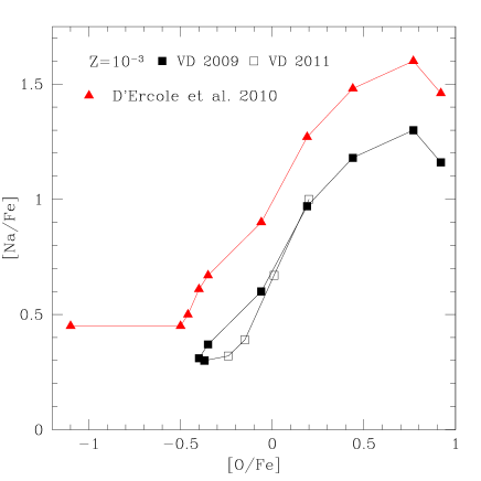
Figure 1: The yields of metallicity Z=10^-3 from Ventura & D’Antona (2009) from AGB models are plotted as full black squares. Masses from top to bottom are 3, 3.5, 4, 4.5, 5, 5.5, 6 and 6.3$\,{M}_{\odot}$. Yields from Ventura & D’Antona (2011) for super–AGB models of 6.5, 7, 7.5 and 8$\,{M}_{\odot}$ are plotted as open black squares. Red triangles represent the yields adopted in D’Ercole et al. 2010: masses are 3, 3.5, 4, 4.5, 5, 5.5, 6, 6.3, 6.5 and 9$\,{M}_{\odot}$.

2.1 Sodium

By increasing the initial mass from 3$\,{M}_{\odot}$ to 8$\,{M}_{\odot}$, the Na and O values provided by the models ejecta first decrease, reach a minimum value in the yields (at masses $\sim$6.5$\,{M}_{\odot}$), and then they both revert back toward higher values. Notice that the location in the Na–O plane of the yields of super–AGBs for the masses 6.5$\leq$M/$\,{M}_{\odot}$$\leq$8 is not different from that of stars with lower masses, it is simply reversed. This behaviour is due to the huge mass loss rates of super–AGBs (Ventura & D’Antona, 2011) and differs from the values adopted in D2010 in which the last point in the yield table was taken to be at very low oxygen ([O/Fe]=–1) and moderate sodium.

The comparison between yields and the data for single-metallicity GCs clearly shows that to reproduce the observed Na–O anticorrelation it is necessary to dilute the AGB ejecta with pristine gas (Bekki et al., 2007; D’Antona & Ventura, 2007; D’Ercole et al., 2008, 2010).

Although the yields of massive stars do not show the strong direct correlation of Na and O, but a moderate anticorrelation, dilution is also needed in models based on the FRMS ejecta (Prantzos & Charbonnel, 2006; Decressin et al., 2007; Lind et al., 2011), and seems to be present in all clusters. Detailed hydrodynamical models able to explain the dynamics and the presence of pristine gas during the SG formation are still lacking. The issue of dilution is discussed in detail by D’Ercole et al. (2011).

The Na abundances adopted in D2010 are +0.3 dex larger than the values reported in Ventura & D’Antona (2009) and adopted in the present work. This assumption was necessary to succesfully reproduce the observed anticorrelations, and was theoretically justified by assuming a 50% increase in the ²⁰Ne(p,$\gamma$) reaction rate and a larger ²⁰Ne abundance in the initial gas mixture. In the present work, use of super–AGB yields makes this adjustment necessary only for the specific case of M 4 in which a ²⁰Ne overabundance is actually present (see Sect. 3).

2.2 Oxygen

The computed super–AGB models show that the sodium and oxygen yields increase with the mass, and that [O/Fe] never reaches values smaller than $-0.4$ (cf. Table 1 and Fig. 1). This behaviour raises a question on the origin of the very low oxygen abundances ([O/Fe]$\sim-1$) found in the giants of some clusters (these are the stars classified as Extreme second generation by Carretta et al. 2009a). We propose to solve the issue with a single additional assumption. We attribute the very small oxygen abundances to an “in situ” deep–mixing, acting only in the progenitors having a very high helium content. In these stars, the small molecular weight discontinuity during the red giant branch evolution may not be able to preclude deep-mixing and lowering of oxygen in the envelope. Stars having the largest helium abundances would then signficantly reduce their atmospheric oxygen content, while preserving a similar sodium abundance (D’Antona & Ventura, 2007). The presence of [O/Fe] abundances smaller than those predicted by AGB models only among the giants, and not among the turnoff or subgiant stars so far examined (Carretta et al., 2006), and in stars belonging to clusters also showing the signature of a very helium rich MS, such as NGC 2808 and $\omega$ Cen, are a possible argument in favour of this interpretation. Obviously, the determination of a very low oxygen content —similar to the one in the most anomalous red giants— in the atmosphere of blue MS stars in these clusters would falsify this suggestion (Bragaglia et al., 2010, were not able to measure oxygen in their spectrum of the blue MS in NGC 2808.).

We apply the following deep-mixing scheme to our models: if a population of SG stars is born from the pure ejecta of super–AGB stars and massive AGBs, in which the helium content is Y$>$0.34, we assume that the surface abundances in the atmospheres of the SG giants is due to deep-mixing; as explained above, this has the effect of reducing the oxygen abundance while leaving the Na abundance unaltered.

The following steps are followed: 1) we examine the helium content in the star–forming gas at each time step; this helium content is the average content of the gas reservoir, either due to the super–AGB or AGB ejecta, in absence of pristine gas, or averaged with the re–accreted pristine gas; 2) if the helium content in the star forming gas is Y$>$0.34, we adopt a “deep–mixing” scheme to provide the oxygen content at the surface of giants. In the absence of non parametric models, the relation chosen to fix the oxygen content after the deep-mixing has some degree of arbitrariness. We decided to link the value to the helium abundance of the gas forming the stars. [O/Fe] is linearly interpolated between the values –0.4 and –0.9, assumed respectively for helium content Y=0.34 and Y=0.36. Consequently, when the ejecta of the mass 7.5$\,{M}_{\odot}$ form stars, they will reach the minimum oxygen values when evolving as giants. We assume: [O/Fe]=–0.4–(Y–0.343)$\times 37.5$. We point out that this expression is adopted as an example only, and other –arbitrary– formulations could have been chosen. 3) if the average helium abundance is smaller than the values for which deep-mixing occurs, the [O/Fe] of the SG stars is equal to the average between the standard [O/Fe]$\sim$0.4 of the pristine matter, and the mildly depleted [O/Fe] of Table 1.

This unique assumption on the simulations will change dramatically our understanding of the O–Na anticorrelation in clusters that do not show extreme anomalies.

2.3 Magnesium and Aluminum

As for magnesium and aluminum , in this paper we adopt the yields obtained in our standard models (Ventura & D’Antona, 2009) in which the NACRE upper limits for the aluminum production by proton capture on ²⁵Mg and ²⁶Mg (Angulo et al., 1999) are used. The super–AGB computations have shown that the maximum Mg depletion is achieved in models of 5–6$\,{M}_{\odot}$, and not in the super–AGB models, contrary to the extrapolation suggested in D2010. The extent of possible variation of Mg and Al yields by varying the input physics is discussed in Ventura, Carini & D’Antona (2011).

2.4 Helium

As discussed in the literature (Ventura et al., 2002), the helium abundance in the ejecta of massive AGB stars is mainly due to the second–dredge up, as the thermal pulse phase in the mass range of interest for the formation of the second generation is so short that the episodes of third dredge up do not increase significantly the value achieved at the second dredge up. The same happens in super–AGB stars, whose evolution is faster than that of massive AGBs and whose thermal pulses are less energetic and less effective for what concerns the third dredge up. Therefore, the helium yield of super–AGB stars, contrary to what happens for the other chemical elements of interest here, does not depend on the assumptions made for the mass loss rate. The average helium abundance increases steadily with the mass, reaching a maximum value of mass fraction Y=0.359 for the 7.5$\,{M}_{\odot}$model. In the 8$\,{M}_{\odot}$ evolution, the total helium in the ejecta is down to Y=0.344. As discussed in Ventura & D’Antona (2011), this is due to the different behaviour of this model, that ignites carbon in the core before the second dredge up. Although the results of the 8$\,{M}_{\odot}$ evolution must be taken with caution for what concerns the other elemental abundances, that dramatically depend on the huge mass loss suffered by this model (following the choice made in Ventura & D’Antona, 2011, for the formulation of the mass loss rate), it is difficult to think that a decrease of the second dredge up effects is physically motivated. Therefore, these models can not explain the Extreme multiple generations of GCs, if we have to take at face value the helium contents Y$>$0.38 that compete to the blue main sequences (Norris, 2004; Piotto et al., 2007) or even the value Y$\sim$0.42 attributed to the blue hook stars in NGC 2419 by di Criscienzo et al. (2011). We follow this line of reasoning: we must not take at face value neither the fit of observations with models (see, e.g., the alternative interpretation by Portinari et al., 2010, on the Y values to be attributed to the helium rich main sequence) nor the mediated proposals of precise very large values of Y from the analysis of the horizontal branch stars, as often pointed out by the same authors (D’Antona & Caloi, 2008), but only the existence, in these clusters, of well defined helium rich sequences. In the absence of direct measurements of the helium abundance, we will assume that the average value of Y of our super–AGB models is more than adequate to describe the Extreme populations of these clusters. Notice that Siess (2010), in spite of using different physical inputs, reaches a maximum value (Y=0.375) in his super–AGB models of the same metallicity. Other models in the literature (e.g. Boothroyd & Sackmann, 1999; Doherty et al., 2010; Lagarde et al., 2011) reach values of helium abundance in the same range (Y$\sim$0.33 – 0.38), in spite of differences in codes, numerical inputs and physical approaches in the mixing formulation (see for discussion Ventura 2010 and D’Antona, Charbonnel et al. 2012, in preparation).

Table 2: Dynamical input parameters for the simulations

Cluster	Model	SG formation	$t_{\rm acc}$(a)	$\tau_{\rm pri}$	$t_{\rm end}$	$(t_{\rm f}$) $\delta t$(b)	$\rho_{\rm*,FG}$	$\rho_{\rm 0,pr}$	$\nu$	$x$
			(Myr)	(Myr)	(Myr)	(Myr)	$\,{M}_{\odot}$pc-3
M 4	0	continuous	65	2	105		9.4	0.091	0.1	0.7
M 4	1	continuous	43	1	100		60	0.085	0.1	0.5
M 4	2	continuous	43	2	60		940	0.05	0.1	0.5
M 4	3	accum.	43	2	50	(45)	940	0.04	0.5	0.5
M 4	4	accum.	43	2	55	(45)	940	0.04	0.5	0.5
M 4	5	accum.	48	10	58	(48)	940	0.08	0.5	0.5
NGC 2808	0	continuous	58	6	68		240	0.01	1	0.5
NGC 2808	1	continuous	65	8	90		240	0.0095	1	0.4
NGC 2808	2	accum.	65	8	90	(50)	240	0.0095	1	0.4
NGC 2808	3	bursts	87	10	100	50-80	240	0.0045	1	0.4
NGC 2808	4	bursts	87	10	90	50-80	240	0.0045	1	0.4
NGC 2808	5	bursts	87	10	90	50-80	240	0.02	1	0.4

^(a) times in Myr.

^(b) $t_{\rm f}$: time until which the AGB ejecta are accumulated before star formation begins

^(b) in models N2808–3, 4 and 5 we list $\delta t$, the time interval during which there is no star formation.

3 The chemical evolution model

The chemical evolution is computed following equations 2–5 of D2010. According to the framework presented in D2010, FG stars are already in place and have the same chemical abundances of the pristine gas from which they form; the SG stars form from super–AGB and AGB ejecta gathering in the cluster centre through a cooling flow and partially diluted with pristine gas accreting on the cluster core with (possibly) a time delay with respect to the beginning of the SG formation epoch.

In order to preserve the cooling flow, we still assume that only SG stars that do not explode as SN II can form (D’Ercole et al., 2008). Another reason to exclude the SG SN II is that normally GCs show a very small spread of iron (Carretta et al., 2009c), indicating that the SG stars hardly have been polluted by SN II ejecta (neither of the FG nor of the SG). The parameters characterizing the model are the same ones listed in D2010:

1. $t_{\rm acc}$: time at which the maximum accretion of pristine matter occurs;

2. $\tau_{\rm pri}$: timescale of the pristine gas accretion process;

3. $t_{\rm end}$: time at which the SG star formation ends;

4. $\rho_{\rm{*,FG}}$: densiy of FG stars;

5. $\rho_{\rm{0,pr}}$: densiy regulating the amount of available pristine gas, normalized to $\rho_{\rm*,FG}$;

6. $\nu$: star formation efficiency

7. $x$ = $\rho_{{\rm*,SG}}/\rho_{{\rm*tot}}$: ratio between the SG stars and the total nowadays alive stars ($\rho_{{\rm*,tot}}=\rho_{{\rm*,FG}}+\rho_{{\rm*,SG}}$)

An exploration of this whole set of parameters has been presented in D2010. In the following we will vary only the most critical parameters ($t_{\rm acc}$, $\tau_{\rm pri}$, $t_{\rm end}$, $\nu$ and $\rho_{\rm 0,pr}$). Notice that $t_{\rm end}$ is not necessarily linked to $t_{\rm acc}$ and $\tau_{\rm pri}$, as the phenomenon causing the end of the SG star formation (e.g. the phase of type I supernova explosions, cf. D2010) is not related. The ratio $x$, in most GCs, is larger than 0.5 (D’Antona & Caloi, 2008; Carretta et al., 2009a). This current value depends not only on the duration and efficiency of the star formation of the SG, but also on the subsequent loss of FG stars (see, e.g. D’Ercole et al., 2008). Although the loss of FG stars does not enter directly into the models (it is in fact absent in equations 2–5 of D2010), its value can be inferred a posteriori from the fit of specific data for the clusters. In the examples of Sect. 4 we adopt $x=0.4$ or 0.5 for NGC 2808 and $x=0.5$ or 0.7 for M 4.

The initial values for the pristine gas abundances can be inferred from the observed data. For example, the initial Mg and Al abundances in the cluster M 4 must be consistent with the observed values [Mg/Fe]=0.5 and [Al/Fe]=0.5, while we adopt more standard values of [Mg/Fe]=0.3 and [Al/Fe]=0 for the initial abundances in NGC 2808. M4 FG stars also exhibit a small increase ($\sim+0.05$dex) in the initial oxygen content. This calls for a variation of the Mg and Al abundances of the AGB ejecta given in Table 1, as these latter are computed for the initial values [Mg/Fe]=0.4 and [Al/Fe]=0. Magnesium and Aluminum were modified on the basis of the details of the various channels of the Mg-Al nucleosynthesis, discussed in Ventura, Carini & D’Antona (2011). The change in the oxygen yields is simpler, because this element is destroyed with continuity during the whole AGB phase, which allows a straight scaling relation. Further, the overabundance of $\alpha$-elements in M 4 should also imply an overabundance of neon. Adopting the relation discussed in D2010 for the sodium production by AGB stars ($\delta$ [Na/Fe]$\simeq\delta$[²⁰Ne/Fe]), we increased the sodium yield values of Table 1 only for the specific case of M 4. Table 3 summarizes all the variations adopted in our models.

Table 3: Chemical input parameters for the simulations

Cluster	$\delta$[O/Fe]	$\delta$[Na/Fe]	$\delta$[Mg/Fe]	$\delta$[Al/Fe]	Oin	Mgin	Alin
	(a)	(a)	(a)	(a)	(b)	(b)	(b)
M 4	0.05	+0.21	+0.03	+0.05	580	60	6
NGC 2808	0.0	0.0	-0.05	-0.10	580	40	2.5

⁽¹⁾ for all the M 4 models but M 4-0, for which $\delta$[Na/Fe]=0.3.

^(a) difference in the AGB yields with respect to Table 1.

^(b) mass fraction of the element in the pristine gas, in units of 10^-6.

4 Results: M 4

4.1 Continuous star formation

In D2010 we presented a model to fit the M 4 O–Na and Mg–Al data by Marino et al. (2008). In Fig. 2 we reproduce a model with the same dynamics (M 4-0 in Table 2) but with the abundances calculated using the new Table 1 (and Table 3). The bottom right panel shows the role of ejecta (dash–dotted line) and of the pristine gas accretion (long–dashed line) and their timing in the detailed formation of the SG (dashed line). The bulk of the SG formation occurs when the pristine matter is re-accreted, at $\sim$65 Myr, and lasts for $\sim$40 Myr more. The dashed lines in the left panels show the path of the O–Na and Mg–Al abundances along the simulation. We see that, when dilution with pristine matter sets in, the values tend towards the FG abundances. As we discussed in D2010, this choice of input parameters provides agreement with the data if the sodium abundance is assumed to be larger by +0.1 dex, with respect to the yields adopted in that work, that is, larger by +0.3 dex with respect to Table 1. As discussed in Sect. 2.1, this would mean to assume that the neon abundance in the gas forming the FG stars of M 4 is +0.3 dex larger than in other cluster–forming regions, in particular in NGC 2808, for which we used directly the values in Table 2. The top right panel of Fig. 2 shows the helium distribution. The total spread is $\delta$Y$\sim$0.04, and could be revealed by a careful analysis of the MS.

The new super–AGB yields broaden the range of possible star formation routes that can satisfactorily fit the M 4 data, showing that different re-accretion histories may lead to similar mild O–Na anticorrelations found in numerous GCs. In the new models star formation can begin much earlier: a first example is shown in Fig. 3 (case M 4-1). The star formation efficiency in this model has still the low value $\nu$=0.1 assumed in the previous case, and no star forms directly from super–AGB ejecta (as we see from the distribution of the helium abundance). Here (and in all the following models of M 4) the adopted excess of sodium abundance is reduced to $\delta\rm{[Na/Fe]}=0.2$, and we assume $x$=0.5 instead of 0.7 considered in the previous model for the sake of comparison with the model of D2010. A fraction of 50% of FG stars is in fact consistent with the fraction of red HB stars given in Marino et al. (2008). Recent analysis of UV based colors of the red giants actually show that the RG branch is splitted into a Na–rich (redder) and Na–normal (bluer) part, in balanced numbers (Milone 2011, private communication).

Model M 4-1 requires the presence of pristine gas since the early phases of SG formation to efficiently dilute the super–AGB matter. Thus the strong dilution of the high–helium super–AGB ejecta leads to helium abundances not much larger than the pristine helium abundance in the gas forming the SG. As discussed in Sect.2.2, the oxygen content is not reduced by deep-mixing: the SG ends up forming a group of stars with relatively large sodium (also thanks to the inclusion of $\delta$[Na/Fe]=+0.2 in the yield table, as discussed above), but with oxygen depleted only by $\sim$0.1 dex. The small helium spread shown by this simulation is probably undetectable on the main sequence, but can lead to a distribution of the HB stars such that the Na–rich stars are bluer than the Na–normal stars, as found by Marino et al. (2011).

We also run the model M 4-2 (Fig. 4) to illustrate how acceptable solutions can be obtained even for significantly shorter evolutionary times. This shows that this kind of models are flexible enough to reproduce the observations in a variety of conditions; this also means, however, that these models can provide only limited constraints on the gas hydrodynamics and the related star formation history.

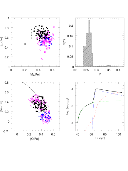
Figure 2: Simulation for the SG of M 4, following the criteria of D2010 (case M 4-0). The top-left panel and the bottom-left panel show the [Mg/Fe]-[Al/Fe] and the [O/Fe]-[Na/Fe] diagrams, respectively. Data (open circles) are from Marino et al. (2008). Squares and triangles represent a sampling of the SG and FG stars by our model, respectively.The dashed lines represent the gas trajectory within the diagrams; the sampled stars in principle would be located on this line, but we introduced a random scatter in the range 0.1 dex in their coordinates in order to mimic the observational errors. The top-right panel illustrates the stellar He distribution. In the bottom-right panel the evolution of the following quantities is reported: total amount of gas (solid line), stellar ejecta (dot-dashed line), pristine gas (long-dashed line), SG stars (dashed line).

Figure 3: Model M 4-1. In this model the pristine gas accretion is greately anticipated with respect to the model M 4-0 of Fig. 2 (symbols as in Fig. 2).

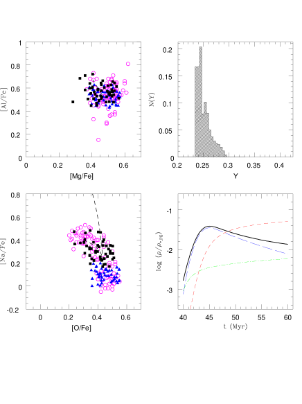
Figure 4: Model M 4-2. The strong, early dilution or super–AGB ejecta with pristine gas allows the formation of the SG at early times aftr the end of the SN II epoch (symbols as in Fig. 2). The time evolution is much shorter compared to models M 4-0 and M 4-1.

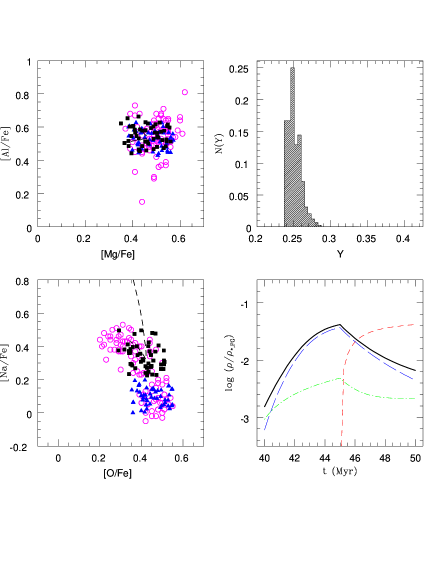
Figure 5: Model M 4-3. The pristine gas and super–AGB ejecta accumulate and a short–lasting burst of star formation occurs at 45 Myr (symbols as in Fig. 2).

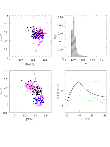
Figure 6: Model M 4-4. The same input parameters of model M 4-3, but the evolution lasts for 5 Myr longer, when the pristine gas is already exhausted, and a tail of helium–rich stars is formed from pure AGB ejecta (symbols as in Fig. 2).

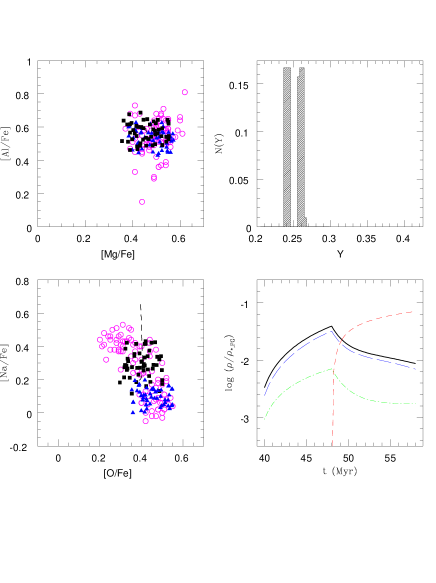
Figure 7: Model M 4-5. The burst of star formation occurs after accumulation until an age of 48 Myr: FG and SG stars are born with a finite, although very small, difference in helium content (symbols as in Fig. 2).

4.2 Star formation after gas accumulation

In Fig. 5 we model a different case (M 4-3). Here we adopt $\nu$=0.5, and let the super–AGB ejecta and pristine gas accumulate up to an age of 45 Myr, when a burst of formation occurs, lasting until a total age $t_{\rm end}$=50 Myr. The process of SG formation must stop very soon with these parameters.

In Fig.6 (case M 4-4), we assume $t_{\rm end}$=55 Myr, and a small tail of stars with larger helium content (and lower [O/Fe]) is formed from pure AGB ejecta in the time interval 50–55 Myr; such a tail is not present in the data, but it is possible to increase $\tau_{\rm pri}$ to avoid this problem. Our aim here is to show how much a small variation of the input parameters may lead to different results, when SG stars form from super–AGB ejecta, i.e. when, contrary to model M 4-0, shorter evolutive times are involved.

To further illustrate this point, we show another simulation in Fig. 7 (Case M 4-5), with a longer timescale for the SG formation. Interesting to notice, the helium content of the SG is again only slightly increased, but here it is well separated from the FG value. Possibly, a careful color analysis of the main sequence width following the lines described, e.g., by Milone et al. (2011a) could reveal this bimodality in helium abundance, and discriminate between this model and the previous one. Models similar to this one may be able to reproduce the abundances in other clusters showing a bimodal HB.

4.3 Which model is more adequate?

Thus, there are two main different modalities in which the AGB pollution may lead to a viable model for M 4: either the re-accretion of pristine gas is delayed by more than 20 Myr (model M 4-0 and D2010), or it occurs early after the SN II epoch (models M 4-2 and following). The choice between these possibilities can rely upon the distribution of other elemental abundances in the FG and SG. In particular, the model M 4-0 shows a small increase in the aluminum abundance of the SG (Fig. 2, top left panel). Marino et al. (2008) data, and also the recent data by Villanova & Geisler (2011), do not show a clear aluminum trend. In addition, the D2010 and M 4-0 models show a finite spread in the helium abundance of the two populations, and model M 4-5 a bimodality in the helium content.

The helium abundance may offer another possible way to choose among the models, by examining the morphology of the HB, and the abundances of sodium and oxygen at different locations along the HB. Originally, D’Antona et al. (2002) proposed to explain the color spread in the HB of most GCs not as an effect of a mass loss spread, as generally thought, but as an effect of helium increase from the cooler to the hotter side. At a given age, the mass of stars evolving off the main sequence is smaller for larger helium abundances. This implies that, for a similar mass loss, stars with a larger helium abundance end up with a smaller mass and thus at a bluer location on the HB. Depending on the metallicity, a very small helium increase (from Y=0.24 to Y$\simeq$0.27) is necessary to produce the gap —a real lack of stars in the RR Lyr region— between the red clump and the blue HB in NGC 2808 (D’Antona & Caloi, 2004). In clusters like M 4, having a more continuous distribution between red and blue, with the presence of several RR Lyr stars, the helium variations may have been less abrupt. Marino et al. (2011) found that the blue HB stars of M 4 have high Na, while the red HB stars have normal Na. Furthermore, Villanova et al. (2012) have recently observed six blue HB stars in M 4, finding that they have high Na, low O and helium content Y$\sim$0.29. A similar location of Na–rich, O–poor stars at the blue side of the HB has been recently discovered by Gratton et al. (2011) in NGC 2808, confirming the scenario. We remark that this same analysis shows a mild anticorrelation of the color with the Na/O ratio within the red clump stars, so that, contrary to the simple interpretation, even the red side of the HB may be not fully populated by FG stars, but also by a few SG stars having a helium content barely larger than the FG value. Also in NGC 1851 Gratton et al. (2012) have found a few Na-rich stars at the hotter end of the red clump. These cases show that extreme care is necessary before drawing firm conclusions on the number ratio of FG to SG stars from simplified analyses. .

Figure 8 illustrates the different ways in which helium is correlated to sodium in our simulations. While in model M4-0 the difference in helium between SG and FG stars is $\delta$Y$>~{}0.02$, other models have a population of SG stars at Y$\sim 0.25$ (model M4-2) or 0.255 (model M4-4). Model M 4–5 shows that it is possible to obtain a mono–helium SG (in our case Y$\sim$0.26) with a large sodium spread. From these examples, it appears that the models employing the super–AGB may be able to explain the presence of SG stars on the blue side of the red clump of NGC 1851 (see Sect. 5 for the case of NGC 2808). Quantitative simulations of the HB in this and other clusters might help to determine which of the models presented is the best. While these simulations are outside the scope of this paper, we point out that the models presented can potentially explain a variety of different HB morphologies and can be tested by spectroscopic observations similar to those by Marino et al. (2011); Villanova et al. (2012).

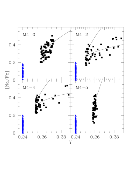
Figure 8: Sodium versus helium abundance in the labelled simulations. The line represents the Y–Na temporal path of the model yields during the formation of the SG. As for other figures, the number of points along different portions of the lines is proportional to the star formation rate (symbols as in Fig. 2).

We summarize these results by concluding that:

1. The mild O–Na anticorrelation and the small – if any – variation in helium shown by a class of GCs can be due to pollution of super–AGB stars into the re–accreted pristine gas forming the second generation stars. The needed ingredient is that the pristine matter falls back to the cluster core very soon after it has been totally removed from the cluster, during the FG SN II epoch.

2. Another important outcome of the simulations including the super–AGB ejecta is that the SG formation phase can have a short duration ($\sim$ 10-20 Myr) and does not need to extend up to $\sim$ 100 Myr (as found by D2010). The models characterized by a shorter SG formation epoch, on the other hand, require a larger star formation efficiency. Models with a short SG formation phase can be compatible with a second phase of SN II explosions due to the evolution of SG massive stars, thus relaxing any assumption of anomalous IMF.

3. As an aside of the previous point, we stress that a shorter SG formation implies that the mass range of the AGB progenitors providing polluted ejecta for the SG formation is narrower and, therefore, that these models require a more massive FG cluster to be able to produce the observed amount of SG stars. Models with a short SG formation phase typically require an initial FG mass 3–4 times larger than that needed in models with a more extended SG formation phase.

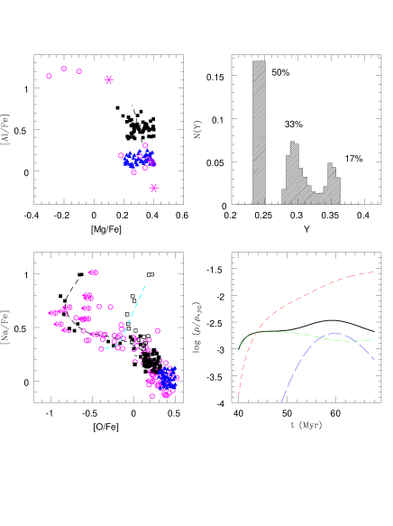
Figure 9: Results for the model NGC 2808-0. Data for giants (open circles) are taken from Carretta et al. (2009a, 2009b). The two turnoff stars examined by Bragagliaet al. (2010) are shown in the Mg–Al panel with star symbols. The open squares in the O–Na panel represent the location of stars formed from ejecta with Y$>$0.34 in absence of deep-mixing (e.g. for the blue MS turnoff stars). The remaining symbols are as in Fig. 2. The top right panel shows the histogram of the helium distribution, with relative number fractions in evidence.

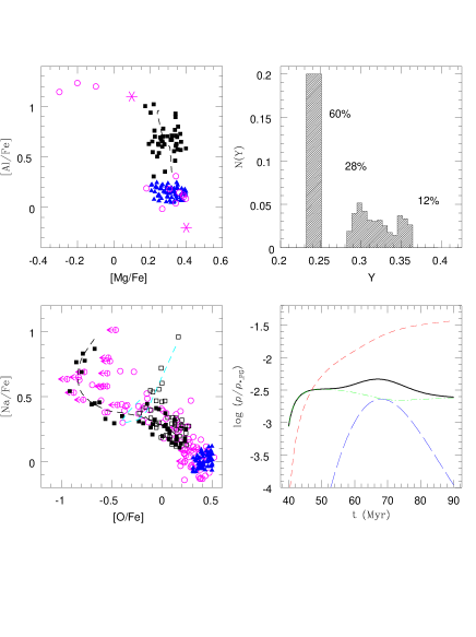
Figure 10: As Fig. 9, but for model NGC 2808–1.

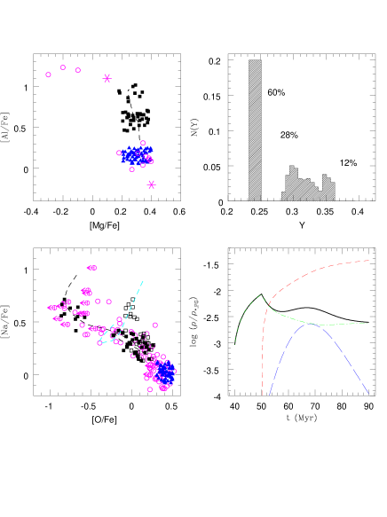
Figure 11: Results for the model NGC 2808–2 . The parameters are the same as to those of model NGC 2808-1 in Fig. 10, but the super–AGB ejecta are assumed to accumulate without forming stars until $t=50$ Myr, as can be seen from the bottom right panel (symbols as in Fig. 9).

5 Results: NGC 2808

We model NGC 2808 by taking it as the prototype of clusters with an extended Na–O anticorrelations, along the lines described by D’Ercole et al. (2008) and in D2010. This means that we do not attempt to model the recent observational details in the analysis of the red HB stars, shown by Gratton et al. (2011), and consider only the formation of two main populations: an extreme one, born from super–AGB undiluted ejecta, and a milder one, born after dilution with the re–accreted pristine gas.

5.1 Continuous star formation

Figure 9 shows the model NGC 2808-0 which has a set of parameters very similar to that for the model of NGC 2808 illustrated by D2010. After the phase of formation from super–AGB ejecta, the peak value of re–accretion occurs at $t_{\rm acc}$=58 Myr (cf. the bottom right panel). The epoch from 38.9 to $\lower 2.15277pt\hbox{$\;\buildrel>\over{\sim}\;$}\sim$50 Myr corresponds to the formation of the Extreme population, with Y$\sim$0.35. This accounts for the presence of the blue main sequence. The following dilution phase leads to the formation of a less extreme SG (Y$\sim$0.3) that populates the intermediate main sequence of this cluster.

The top left panel of figure 9 shows the Mg and Al predictions. Using the new yields for Mg and Al listed in Table 1 does not allow the fit of the three Mg–poor giants ($\delta$[Mg/Fe]$\sim$–0.6) observed by Carretta et al. 2009b. Ventura, Carini & D’Antona (2011) deal extensively with the Mg–Al problem in the models, and show that small adjustments to the cross sections (concerning the Mg isotopes) may well reproduce the [Mg/Fe]–[Al/Fe] value of the blue MS stars observed by Bragaglia et al. (2010) and shown in Fig. 9 with the star symbol. In particular, an increase by a factor two of the cross section ²⁵Mg(p,$\gamma$)²⁶Al shifts the 6$\,{M}_{\odot}$ yield in the region occupied by the M 13 giants and by the MS star of NGC 2808. Such an increase is also consistent with recent new measurements of the reaction rate (LUNA Collaboration et al., 2011).

The difference in Mg between the MS stars and the giants can not be attributed to further dilution in the red giants, as magnesium is not touched in the red giant evolution of low mass stars, not even in the interior (D’Antona & Ventura, 2007). Figure 5 in Ventura, Carini & D’Antona (2011) shows the Mg–Al data in the literature for the clusters NGC 6752, M 15, NGC 2808 and M 13, and the results of different modeling of the yields in the chemistry evolution of a 6$\,{M}_{\odot}$ star as adopted in this paper. Apart from two giants in M 15, a cluster whose metal abundance is much smaller than the others, no star has Mg abundances as low as those in the three UVES giants of NGC  2808, that are not compatible with the models. As these three stars constitute a problem for any other pollution model, and can not be explained in the deep extra mixing framework as well, we defer the study of this problem to a future investigation.

Let us now consider the [Na/Fe]-[O/Fe] diagram (bottom left panel of Fig. 9). While in the case of M 4-0 the new simulation is very similar to that presented in D2010 for the absence of an Extreme population, here the new super–AGB sodium yields are able to account for the high sodium values of the stars with upper limit only available for oxygen (full squares); this results ensues from the deep-mixing hypotesis, and the subsequent reduction of the oxygen values given by the recipe described in Sect. 2.2. The open squares represent the values of oxygen that should be found in turnoff stars for the stars with Y$>$0.34, as in these stars deep-mixing has not yet taken place. These stars, as well as blue MS stars, should be characterized by oxygen abundances larger than those of giant stars and fall along the Na-O curve determined by the new yields and shown in Fig. 1, a prediction that can be falsified by spectroscopic observations.

The top right panel of Fig. 9 shows the histogram of the distribution of helium abundances. The number ratio of the Intermediate and Extreme populations of the SG depends on the initial mass function and on the timing and extent of the dilution with pristine gas, and thus this is a powerful constraint for the successful models. The observed number ratios of the three populations differing in helium content in NGC 2808 is constrained by two different sets of observations:

1. the number counts of the HB stars (Bedin et al., 2000). These numbers were the basis of the interpretation of the HB in terms of multiple populations with different helium content (D’Antona & Caloi, 2004; D’Antona et al., 2005), providing fractions of 50%, 35% and 15%, respectively, for the groups of standard helium (red clump stars), intermediate helium (blue luminous HB, named EBT1) and high helium (sum of the EBT2 and EBT3 extensions of the blue HB).

2. the number counts in the triple MS. Milone et al. (2011b) recently re–analyzed the data by Piotto et al. (2007) in order to derive the mass functions of the three populations. According to this analysis, the fractions of standard (red MS), intermediate (middle MS) and high helium (blue MS) stars are respectively 62%, 24% and 14%. Therefore, while the fraction of FG stars changes from $\sim$50 to $\sim$60%, the proportion of Intermediate and Extreme population are very similar in the two analyses: the Extreme population is $\sim$35% of the whole SG.

In the present models for NGC 2808 we set $x=0.4-0.5$, that is, we assume that the fraction of FG stars, with standard helium content Y=0.24, is 60-50%, and set the other input parameters in order to obtain a reasonable result for the number ratio of the Extreme and Intermediate SG.

From the above discussion it is clear that, contrary to the case of M 4, there is less freedom in the choice of the parameters because of the presence of the Extreme population and the need to reproduce the right proportion among the Extreme, the Intermediate and the Primordial populations (cf. the three peaks in the He histogram in Fig. 9). Some degree of flexibility is still present though. Figure 10 shows another model for NGC 2808, whose input is model NGC 2808-1 in Table 2. In the left panels we see that, as for the model NGC 2808-0, when dilution with pristine matter sets in, the model trajectories (dashed line) tend towards the FG abundances, but, during the last 10–15 Myr, star formation occurs again in mostly undiluted AGB ejecta, and the abundances revert back to lower O and larger Na values. In fact, this last phase of star formation is necessary to fill the gap in O, Na values between the formation of the Extreme population (with very large Y, corresponding to the blue MS) and the Intermediate population with strong dilution. The bump in the helium distribution between the peaks at Y=0.3 and Y=0.35 (top right panel) forms during this same stage as well. And also the stars with very large [Al/Fe] in the simulation (upper left panel) form in this last epoch of star formation. This can be understood by looking at the abundances listed in Table 1, showing that the maximum abundance in Al and maximum depletion in Mg are reached with the evolution of the 5.5$\,{M}_{\odot}$(at about 85 Myr).

5.2 Star formation after gas accumulation

We now focus on Fig. 11 that shows the results of the model NGC 2808–2, having the same input parameters of model NGC 2808–1, but dealing with a different hypothesis for the star formation: here we assume that SG formation does not start immediately after the end of the SN II epoch, but that gas accumulates from 40 to 50 Myr, and then a star formation burst occurs.

The results are very similar, but the Extreme population does not reach the high sodium abundances obtained in the model NGC 2808–1; this is a consequence of the fact that, before the SG formation starts, the ejecta of the stars between $8\,{M}_{\odot}$ and $\sim$7.3$\,{M}_{\odot}$mix, so that the highest abundances are lowered.

5.3 Models with interruption of star formation due to SG SN II explosions

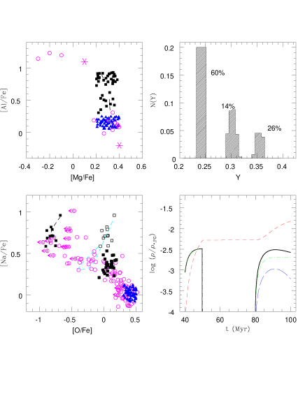
Figure 12: Case NGC 2808-3. Star formation is interrupted for 30 Myr, but the second stage of star formation lasts for 20 Myr (symbols as in Fig. 9).

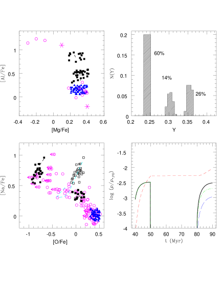
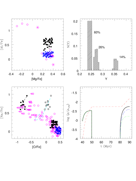
Figure 13: Case NGC 2808-4 (top) and 5 (bottom). Using the input parameters of Fig. 12, but limiting the second star formation phase to 10 Myr, the Intermediate population is very scarce (top panel). Increasing the infall of pristine matter, the O–Na data come very close to the FG values (bottom panel) (symbols as in Fig. 9).

As discussed in Sect. 4, an interesting implication of clusters like M 4, with a short [O/Fe]-[Na/Fe] anticorrelation, is that thay can form the bulk of the SG population in $~{}10$ Myr, or even less; such a timescale is compatible with the survival of a cooling flow in the cluster core, previous to the explosion of the Type II SN of the second generation, and thus there would be no reason to limit the IMF of the SG to the stars that do not explode as SN II.

Understanding whether the formation of two distinct SG populations (such as those found in NGC 2808) is compatible with star formation bursts lasting $\sim$10 Myr is not straightforward. We have tried to model in detail the three populations of NGC 2808 by making the assumption that, $\sim$10 Myr after the Extreme population began to be formed in the cluster, a new phase of SN II begins. This will hamper star formation until the end of the SN II phase.

In our models, this phase lasts for $\;\buildrel<\over{\sim}\;$38 Myr (Table 1). We can have a second burst of star formation from the AGB ejecta starting at $\sim$90 Myr. We have discussed in Sect. 2 that the time hiatus between the two bursts may be reduced to $\sim$30 Myr for models employing a smaller core–overshooting. Thus we employ in the following $\sim$30 Myr as total duration of the SG SN II epoch.

The main difficulty encountered in models including SN II explosions from the Extreme SG is to reproduce at the same time the extension and distribution of stars along the O–Na anticorrelation and the helium distribution function.

• Case NGC 2808-3 (Fig. 12): In this model we stop the SG formation from pure ejecta at 50 Myr, allow for a $\;\buildrel>\over{\sim}\;$30 Myr period without star formation, and then resume star formation from the AGB ejecta mixed with pristine gas, with a choice of $t_{\rm acc}$=87 Myr. The clumps in the distribution of stars in the O–Na plane are probably too separated to be consistent with the observations. Moreover, in order to obtain a reasonable number ratio between the Extreme stars (Y$>$0.34) and the Intermediate population (Y$\sim$0.30), we are forced to extend the star formation of this latter population to $\sim$20 Myr, much longer than allowed by the beginning of the new (third) SN II epoch.

• Case NGC 2808-4 (Fig. 13, top panel): this model is identical to NGC 2808-3, but we limit the formation of the Intermediate population to 90 Myr: as discussed above, the Intermediate population is a bare 11%, too small to reproduce the number ratio of the Extreme– and Intermediate–helium MS.

• (Case NGC 2808-5, Fig. 13, bottom panel): we increase the relative number of Intermediate population stars by increasing the dilution. The second peak of helium content occurs at Y$\sim$0.28, and the number ratio of Extreme and Intermediate population becomes reasonable, but the O–Na values become much too close to the FG values, due to the strong dilution (a problem discussed in D’Ercole et al. (2011) in a different context).

We find then that these simulations do not reproduce the observations so well as models NGC 2808-1 and 2. Nevertheless, the variety of observational results for different clusters may have their explanation in the variety of relevant parameters. For instance, model NGC 2808-4 (Fig. 13 top panel) could be relevant to explain the horizontal branch stellar distribution of the cluster NGC 2419 (di Criscienzo et al., 2011).

6 Conclusions

In this paper we have explored the possible role of super-AGB in the formation of the observed abundance patterns in multiple-population globular clusters. Our models are based on the set of yields calculated by Ventura & D’Antona (2009, 2011). The results of our investigation show that the new super–AGB yields broaden the range of possible formation histories leading to the observed abundance patterns. Specifically:

• we have built models for M 4, a cluster representative of numerous other GCs characterized by a shorter Na–O anticorrelation. For this cluster, we show that the observed abundance pattern can be reproduced also by models with a short SG formation phase ($\sim$ 10-20 Myr) involving only super-AGB ejecta and pristine gas. We confirm that models presented in our previous work (D’Ercole et al. 2010) which are characterized by a more extended SG formation epoch involving super–AGB and AGB ejecta (along with pristine gas) can also reproduce the observed abundance patterns. While models with a shorter SG formation epoch can include the effect of SG SN II, the narrower range of AGB progenitors providing gas for SG formation implies that they require a larger FG initial mass (by a factor 3-4 compared to models with a more extended SG formation phase).

• In order to account for the O-poor Na-rich stars of NGC 2808 we assumed the presence of deep-mixing in SG giants forming in a gas with helium abundance Y$>0.34$, which significantly reduces the atmospheric oxygen content, while preserving the sodium abundance. The use of the super–AGB yields does not change the main requirements on SG formation history of models for the more complex clusters like NGC 2808. In these clusters, an Extreme population with very large helium content form from the pure ejecta of super–AGB stars, followed by formation of an Intermediate population by dilution of massive AGB ejecta with pristine gas. We also attempted to model the three populations of NGC 2808 allowing for a long hiatus between the formation of the Extreme and Intermediate population (possibly due to SN II explosions of the Extreme populations), but our attempts to model each star formation epoch in a period as short as $\sim$10 Myr were not satisfactory. Nevertheless, further study is probably needed to settle this issue.

We finally want to point out that one-zone models such as those presented here (and in D2010), while very useful to understand rather easily and very quickly the role of different ingredients in shaping the GC chemical evolution (AGB ejecta, amount of pristine gas, duration of the system evolution, etc.), cannot of course capture the complexity and variety of effects connected with the gas hydrodynamics. As a simple example, we mention that, during the cooling flow evolution of the GC gas (c.f. D’Ercole et al., 2008), most of it cumulates in the centre of the cluster which therefore at each time hosts not only the AGB ejecta delivered “in situ”, but also that delivered at earlier times by FG stars located at the GC outskirts. It is thus expected that SG stars with different chemical properties can form in different places at the same time, and not only at different times as in one-zone models. For this reason we plan to work out hydrodynamic models similar to those of D’Ercole et al. (2008), but taking into account the detailed chemistry as in the present models.

7 Acknowledgments

We thank Raffaele Gratton for useful comments that helped us to clarify and further expand some of the points presented in the paper. This work has been supported through PRIN INAF 2009 ”Formation and Early Evolution of Massive Star Cluster”. EV was supported in part by grant NASA-NNX10AD86G.

References

- Angulo et al. (1999) Angulo C., Arnould M., Rayet M., et al., 1999, Nucl.Phys. A, 656, 3
- Bedin et al. (2000) Bedin, L. R., Piotto, G., Zoccali, M., et al. 2000, A&A, 363, 9
- Bekki et al. (2007) Bekki, K., Campbell, S. W., Lattanzio, J. C., & Norris, J. E. 2007, MNRAS, 377, 335
- Boothroyd & Sackmann (1999) Boothroyd, A. I., & Sackmann, I.-J. 1999, ApJ, 510, 232
- Bragaglia et al. (2010) Bragaglia, A., et al. 2010, ApJ, 720, L41
- Briley et al. (2002) Briley, M., Cohen, J. G., & Stetson, P. B. 2002, ApJ, 579, L17
- Briley et al. (2004) Briley, M. M., Harbeck, D., Smith, G. H., & Grebel, E. K. 2004, AJ, 127, 1588
- Carretta et al. (2006) Carretta, E., Bragaglia, A., Gratton, R. G., Leone, F., Recio-Blanco, A., & Lucatello, S. 2006, A&A, 450, 523
- Carretta et al. (2009a) Carretta, E., et al. 2009a, A&A, 505, 117
- Carretta et al. (2009b) Carretta, E., Bragaglia, A., Gratton, R., & Lucatello, S. 2009b, A&A, 505, 139
- Carretta et al. (2009c) Carretta, E., Bragaglia, A., Gratton, R., D’Orazi, V., & Lucatello, S. 2009c, A&A, 508, 695
- Carretta et al. (2010) Carretta, E., Bragaglia, A., Gratton, R. G., et al. 2010, A&A, 516, A55
- D’Antona et al. (2002) D’Antona, F., Caloi, V., Montalbán, J., Ventura, P., & Gratton, R. 2002, A&A, 395, 69
- D’Antona & Caloi (2004) D’Antona, F., & Caloi, V. 2004, ApJ, 611, 871
- D’Antona & Caloi (2008) D’Antona, F., & Caloi, V. 2008, MNRAS, 390, 693
- D’Antona et al. (2005) D’Antona, F., Bellazzini, M., Caloi, V., Pecci, F. F., Galleti, S., & Rood, R. T. 2005, ApJ, 631, 868
- D’Antona & Ventura (2007) D’Antona, F., & Ventura, P. 2007, MNRAS, 379, 1431
- Decressin et al. (2007) Decressin, T., Meynet, G., Charbonnel, C., Prantzos, N., & Ekström, S. 2007, A&A, 464, 1029
- D’Ercole et al. (2008) D’Ercole, A., Vesperini, E., D’Antona, F., McMillan, S. L. W., & Recchi, S. 2008, MNRAS, 391, 825
- D’Ercole et al. (2010) D’Ercole, A., D’Antona, F., Ventura, P., Vesperini, E., & McMillan, S. L. W. 2010, MNRAS, 407, 854 (D2010)
- D’Ercole et al. (2011) D’Ercole, A., D’Antona, F., & Vesperini, E. 2011, MNRAS, 415, 1304
- Dickens et al. (1991) Dickens, R. J., Croke, B. F. W., Cannon, R. D., & Bell, R. A. 1991, Nature, 351, 212
- di Criscienzo et al. (2010) di Criscienzo, M., D’Antona, F., & Ventura, P. 2010, A&A, 511, A70
- di Criscienzo et al. (2011) di Criscienzo, M., D’Antona, F., Milone, A. P., et al. 2011, MNRAS, 414, 3381
- Doherty et al. (2010) Doherty, C. L., Siess, L., Lattanzio, J. C., & Gil-Pons, P. 2010, MNRAS, 401, 1453
- Gratton et al. (2001) Gratton, R. G., Bonifacio, P., Bragaglia, A., et al. 2001, A&A, 369, 87
- Gratton et al. (2011) Gratton, R. G., Lucatello, S., Carretta, E., et al. 2011, A&A, 534, A123
- Gratton et al. (2012) Gratton, R. G., Lucatello, S., Carretta, E., et al. 2012, arXiv:1201.1772
- Karakas et al. (2006) Karakas, A. I., Fenner, Y., Sills, A., Campbell, S. W., & Lattanzio, J. C. 2006, ApJ, 652, 1240
- Lagarde et al. (2011) Lagarde, N., Charbonnel, C., Decressin, T., & Hagelberg, J. 2011, A&A, 536, A28
- Lee et al. (2005) Lee, Y.-W., et al. 2005, ApJ, 621, L57
- Leitherer et al. (1999) Leitherer, C., et al. 1999, ApJS, 123, 3
- Lind et al. (2011) Lind, K., Charbonnel, C., Decressin, T., et al. 2011, A&A, 527, A148
- LUNA Collaboration et al. (2011) LUNA Collaboration, Strieder, F., Limata, B., et al. 2011, arXiv:1112.3313
- Marino et al. (2008) Marino, A. F., Villanova, S., Piotto, G., et al. 2008, A&A, 490, 625
- Marino et al. (2011) Marino, A. F., Villanova, S., Milone, A. P., Piotto, G., Lind, K., Geisler, D., & Stetson, P. B. 2011, ApJ, 730, L16
- Meynet et al. (2006) Meynet, G., Ekström, S., & Maeder, A. 2006, A&A, 447, 623
- Milone et al. (2011a) Milone, A. P., Piotto, G., Bedin, L. R., et al. 2011a, arXiv:1109.0900
- Milone et al. (2011b) Milone, A. P., Piotto, G., Bedin, L. R., et al. 2011b, arXiv:1108.2391
- Norris (2004) Norris, J. E. 2004, ApJ Letters, 612, L25
- Pasquini et al. (2011) Pasquini, L., Mauas, P., Käufl, H. U., & Cacciari, C. 2011, A&A, 531, A35
- Piotto et al. (2005) Piotto, G., et al. 2005, ApJ, 621, 777
- Piotto et al. (2007) Piotto, G., et al. 2007, ApJL, 661, L53
- Portinari et al. (2010) Portinari, L., Casagrande, L., & Flynn, C. 2010, MNRAS, 406, 1570
- Prantzos & Charbonnel (2006) Prantzos, N., & Charbonnel, C. 2006, A&A, 458, 135
- Renzini (2008) Renzini, A. 2008, MNRAS, 391, 354
- Schaller et al. (1992) Schaller, G., Schaerer, D., Meynet, G., & Maeder, A. 1992, A&AS, 96, 269
- Siess (2010) Siess L., 2010, A&A, 512, A10
- Smartt (2009) Smartt, S. J. 2009, ARA&A, 47, 63
- Ventura et al. (1998) Ventura, P., Zeppieri, A., Mazzitelli, I., & D’Antona, F. 1998, A&A, 334, 953
- Ventura et al. (2001) Ventura, P., D’Antona, F., Mazzitelli, I., & Gratton, R. 2001, ApJ Letters, 550, L65
- Ventura et al. (2002) Ventura, P., D’Antona, F., & Mazzitelli, I. 2002, A&A, 393, 215
- Ventura & D’Antona (2009) Ventura P., D’Antona F., 2009, A&A, 499, 835
- Ventura (2010) Ventura, P. 2010, IAU Symposium, 268, 147
- Ventura & D’Antona (2011) Ventura, P., & D’Antona, F. 2011, MNRAS, 410, 2760
- Ventura, Carini & D’Antona (2011) Ventura, P., Carini, R., & D’Antona, F. 2011, MNRAS, 947
- Villanova & Geisler (2011) Villanova, S., & Geisler, D. 2011, arXiv:1109.0973
- Villanova et al. (2012) Villanova, S., Geisler, D., Piotto, G., & Gratton, R. 2012, arXiv:1201.3241
- Weiss et al. (2000) Weiss, A., Denissenkov, P. A., & Charbonnel, C. 2000, A&A, 356, 181