Evolutionary accessibility in tunably rugged fitness landscapes

Abstract

The adaptive evolution of a population under the influence of mutation and selection is strongly influenced by the structure of the underlying fitness landscape, which encodes the interactions between mutations at different genetic loci. Theoretical studies of such landscapes have been carried out for several decades, but only recently experimental fitness measurements encompassing all possible combinations of small sets of mutations have become available. The empirical studies have spawned new questions about the accessibility of optimal genotypes under natural selection. Depending on population dynamic parameters such as mutation rate and population size, evolutionary accessibility can be quantified through the statistics of accessible mutational pathways (along which fitness increases monotoncially), or through the study of the basin of attraction of the optimal genotype under greedy (steepest ascent) dynamics. Here we investigate these two measures of accessibility in the framework of Kauffman’s $LK$-model, a paradigmatic family of random fitness landscapes with tunable ruggedness. The key parameter governing the strength of genetic interactions is the number $K$ of interaction partners of each of the $L$ sites in the genotype sequence. In general, accessibility increases with increasing genotype dimensionality $L$ and decreases with increasing number of interactions $K$. Remarkably, however, we find that some measures of accessibility behave non-monotonically as a function of $K$, indicating a special role of the most sparsely connected, non-trivial cases $K=1$ and 2. The relation between models for fitness landscapes and spin glasses is also addressed.

1 Introduction and background

The basic idea of the theory of evolution as presented by Charles Darwin Darwin is that heritable phenotypic variability and the subsequent competition between reproducing organisms (possibly aided by spacial separation of habitats) shape the diversity of life as it can be observed today. This theory, purely descriptive at first, was cast in a quantitative form by Haldane, Fisher and Wright h1931 ; w1931 ; f1930 . This quantification, which is now known as the Modern Synthesis Huxley of evolution founded the field of mathematical population genetics, which has remained an active area of research ever since. As the mutations, i.e. changes to the hereditary material of an organism, which give rise to the diversity in the population, cannot be controlled, they are modeled as random events within the Modern Synthesis. Furthermore, the intricate mechanisms by which the hereditary (or ‘genetic’) information is processed are accounted for in the form of stochastic models, thus methods familiar to statistical physicists find a natural field of application in this context.

Within the Modern Synthesis, populations are subject to four evolutionary forces:

• Selection by relative average growth rate of mutant populations, which is the mechanism by which different mutants compete. Selective forces are quantified by fitness, which is a measure of reproductive success and can be taken to be proportional to the number of offspring an individual leaves in the next generation.

• Genetic drift, which represents random demographic fluctuations due to finite population sampling effects around the deterministic process described by selection alone,

• mutations, which are random changes in the hereditary material, and

• recombination, which corresponds to two individuals combining (parts of) their genetic material in one common offspring.

In this paper, we will focus specifically on the influence of selection on the adaptive fate of a population.

During the last decade or so, the advent of modern technologies has made it possible to directly manipulate or at least inspect the genetic material of model organisms at a molecular level, thus putting the theoretical models of adaptation that have been at the center of attention thus far to the test. Of particular interest is the question of how different mutations interact in their effects on fitness. To give an important example, in s1994 it was found that five mutations in the TEM-1 $\beta$-lactamase gene in the bacterium Escherichia coli together increase the resistance against a particular antibiotic by a factor on the order of $10^{5}$. Besides the obvious clinical relevance of this finding, it raises an interesting theoretical question wwc2005 ; wddh2006 ; ch2009 ; fkdk2011 : Can such a combination of mutations emerge in natural populations, where the five mutations would have to appear and spread one at a time? In other words, is the optimal combination of mutations accessible to the population? In this paper, we will address this problem in two specific regimes of adaptive dynamics.

1.1 Fitness landscapes and adaptive regimes

We start from the common assumption that all the organism’s properties are determined (in a given, fixed environment) by its hereditary information, which is represented as a sequence $\vec{\sigma}=\{\sigma_{1},\sigma_{2},\dots,\sigma_{L}\}$ of length $L$ called the genotype. Real genomes have, at the level of DNA base pairs, four different possible letters or ‘alleles’ at each of the $L$ sites, i.e. $\sigma_{l}\in\{G,A,T,C\}$. If the proteins produced after transcription are modeled Cell , the number of possible alleles goes up to $21$ (the number of amino acids). However, in many cases the number of mutations in a population is small, such that at most two different alleles exist at a given genomic site and the genotype can be modeled as a binary sequence. Thus the fitness $F$ (like all other properties) is a mapping from the Boolean hypercube to the real numbers. A natural measure of distance between any two states is the Hamming Distance (HD) counting the number of point mutations separating two genotypes,

$$d(\vec{\sigma}_{1},\vec{\sigma}_{2})=\sum_{l=1}^{L}(1-\delta_{\sigma_{1,l},\sigma_{2,l}})$$ (1)

where Kronecker’s delta is defined by $\delta_{x,y}=1$ if $x=y$ and $\delta_{x,y}=0$ otherwise. The dynamics of a population on a given fitness landscape (FL) $F(\vec{\sigma})$ can be visualized as a hill climbing process, the statistical features of which depend on the mutation rate $\mu$ per genome, the population size $N$, and the scale $s$ of typical fitness differences. In each new generation, every individual will spawn a number of offspring that is on average proportional to that individual’s fitness. The offspring will, up to mutations, have the same genetic configuration with the same fitness as the parent. Thus the population in general forms a cloud in sequence space. An important early result of theoretical population genetics is that the strength of demographic fluctuations (’drift’) is governed by the inverse population size $1/N$ Gillespie ; Blythe2007 . The parameters $Ns$ and $N\mu$ therefore gauge the strength of selection and mutations relative to the effect of drift, giving rise to different dynamical regimes Park2010 . Two regimes of particular interest in this paper will be described in the following.

1.1.1 The strong selection/weak mutation regime

If the product of population size and mutation rate per individual genome is low, $N\mu\ll 1$, mutations are rare events and the population is genetically homogeneous (‘monomorphic’) most of the time. If furthermore the selection strength is much greater than the strength of demographic fluctuations, $Ns\gg 1$, mutations that lower fitness (called ‘deleterious’) are rapidly driven to extinction. This evolutionary regime is called the ‘strong selection/weak mutation (SSWM)’ regime of adaptation g1983 ; GillespieCauses . In this regime, the population can only move uphill in fitness, and only between states of HD 1. Such a move is then called an ‘accessible step’. Between mutational steps the population is located at one point in sequence space.

1.1.2 The greedy adaptive regime

If selection is still much stronger than drift, but the mutation rate and population size are such that $N\mu\sim L\gg 1$ and $N\mu^{2}\ll 1$, all $L$ states at HD $1$ of the most populated state are generated in one generation, but almost none at greater mutational distance. Since selection is strong, the population will in the next generation be dominated by the most fit of the available $L$ single mutants and continue from that state on. Thus the population can still be localized to a well-defined point in sequence space and the adaptive process takes the route of steepest fitness increase in each step, until a (local or global) fitness maximum is reached. This regime of adaptation is called ‘greedy’ Gillespie ; Orr2003 ; Jain2007 ; Jain2011 .

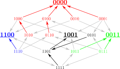
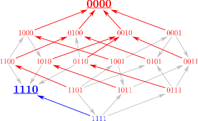
Figure 1: (Color online) Two examples of empirical fitness landscapes obtained from growth rate measurements of different mutants of the fungus Aspergillus niger fkdk2011 ; dhv1997 ; deVisser2009 . The arrows between neighboring configurations point in the direction of fitness increase. Local maxima, i.e. configurations without outbound arrows are underlined. The colors indicate the basins of attraction under steepest ascent (greedy) dynamics. In the left FL the number of accessible paths $n$ from the antipodal genotype $\{1,1,1,1\}$ to the global fitness maximum $\{0,0,0,0\}$ is $n=0$ while in the right example $n=6$

1.2 Topographic properties of fitness landscapes

There are many ways in which the ruggedness or complexity of a fitness landscape can be quantified. Possible measures that have been proposed include the number of local maxima, the length of uphill adaptive walks, or the decay of fitness correlations along a random walk through the landscape Kauffman ; Weinberger1990 ; Stadler1999 . The present work is based on two particular topographic observables which are motivated by the two adaptive regimes described in the preceding sections.

1.2.1 Accessible paths

Within the SSWM regime, the notion of evolutionary accessibility of the optimal genotype can be quantified in a straightforward way wwc2005 : Since the population is constrained to move uphill in single mutations steps, we say that a pathway connecting two genotypes is accessible if each mutation confers a selective advantage, i.e., if fitness increases monotonically along the path. This definition is closely related to the notion of reachability introduced in Stadler2010 . Moreover, since mutations are rare, only the shortest (direct) pathways connecting two genotypes will be considered . For two genotypes at HD $d$, there are $d!$ such pathways corresponding to the different orderings in which the mutations separating them can occur Gokhale2009 .

To obtain a global measure of accessibility, we focus here on pathways to the global fitness maximum which span the entire landscape wddh2006 ; fkdk2011 . If the global maximum is located at a sequence $\vec{\sigma}_{max}$, there is a unique ‘antipodal’ sequence $\vec{\sigma}_{anti}$ such that $d(\vec{\sigma}_{max},\vec{\sigma}_{anti})=L$, and $L!$ shortest pathways connecting it to $\vec{\sigma}_{max}$. Our rationale for using the antipodal sequence as a starting point is that these paths are the longest possible direct evolutionary trajectories on the landscape, and as such their accessibility provides a lower bound on the accessibility of typical paths starting, for example, at a randomly chosen genotypefkdk2011 . On each realization of a FL, a certain number $n$ of these pathways will be accessible in the sense defined above, see fig. 1 for two examples taken from an empirical data set for the filamentous fungus Aspergillus niger fkdk2011 ; dhv1997 ; deVisser2009 . Evolutionary accessibility for an ensemble of FL’s can thus be characterized by the distribution $\pi_{L}(n)$, the probability that in a given realization there will be exactly $n$ accessible paths.

While evolution is constrained to accessible paths only in the SSWM regime, as a topographical feature of a FL, they can be defined independent of any adaptive regime. In this paper, we will analyze the behavior of the distribution $\pi_{L}(n)$ for a particular model of fitness landscapes to be defined in sect. 2.

The study of accessible paths on FL’s can be seen as a kind of percolation problem StaufferAharony on the Boolean hypercube GG1997 ; Gavrilets , with some important differences. In the (bond) percolation problem, individual bonds between adjacent states are open or closed independently of the others, while in the FL context, there is an effective correlation between bonds: Since a bond on a FL is open if the fitness increases when the bond is traversed in the direction towards the global fitness maximum, the states of two bonds adjacent to the same sequence are correlated via the fitness of that state. Moreover, the fact that the accessibility of a bond is determined by the difference of a globally defined fitness function implies a non-local gradient condition (the arrows in fig. 1 cannot form any loops).

1.2.2 Basins of attraction

Assuming a continuous range of fitness values (so that ties cannot occur), evolutionary trajectories under greedy adaptive dynamics are completely deterministic and terminate at local fitness maxima. Thus each genotype $\vec{\sigma}$ is uniquely associated to a fitness maximum that will be reached by a greedy trajectory starting at $\vec{\sigma}$. The set of all configurations leading to a given maximum is called the ‘Basin of Attraction’ (BoA) of that maximum (see fig. 1 for illustration). Under greedy dynamics, the importance of a local optimum can be measured by the size of its BoA. In particular, a landscape where the BoA of the global fitness maximum (GM) $\vec{\sigma}_{max}$ contains a non-vanishing fraction of the FL for large $L$ can be said to be dominated by the GM.

Much like accessible paths, the BoA’s are of direct relevance to the adaptation of a population only if the dynamics take place in the greedy regime defined above, but the distribution of basin sizes can still be considered as a topographical feature and analyzed independently of the adaptive dynamics. Here, the distribution $p_{L}(b_{GM})$ of the size $b_{GM}$ of the BoA of the GM and its expectation value $\langle b_{GM}\rangle$ are studied in the framework of the model of FL’s to be introduced in sect. 2.

1.3 Fitness landscapes and spin glasses

Models of spin glasses (SG’s) were originally introduced in the context of disordered magnets MezardParisiVirasoro and are now used as a paradigm for complex systems across a broad range of disciplines, e.g. in information theory and computational optimization MezardMontanari ; HartmannRieger . There is an obvious close similarity between SG’s and FL’s, since in both cases a real number (energy or fitness) is associated to each configuration of a binary (spin) chain of a given length, and the interest is in complex landscapes with many local minima or maxima Stein1992 .

However, the two classes of systems differ importantly in that the instantaneous state of a spin glass is uniquely described by a single configuration, whereas a biological population generally occupies a cloud in genotype space. A direct comparison between the dynamics of the two systems is therefore meaningful only when mutations are rare, $N\mu\ll 1$, such that the population cloud condenses to a single point in genotype space and adaptive steps occur one ‘spin flip’ at a time. In this regime it can be shown that the effective transition rates between neighboring configurations satisfy detailed balance with respect to an equilibrium measure of Boltzmann form, $P(\vec{\sigma})\sim e^{\lambda NF(\vec{\sigma})}$, with fitness $F$ taking the role of (negative) energy and population size $N$ acting as an inverse temperature Berg2004 ; Sella2005 .

In the spin glass context, the notion of evolutionary accessibility formulated above corresponds to the question of whether the ground state can be reached under a zero temperature dynamics, where only moves that lower the system energy are accepted. Similarly, the size of the BoA of the GM is a measure for the probability that the ground state can be reached through a steepest descent algorithm, which is of interest in the context of optimization theory HartmannRieger .

2 Fitness landscape models

Even though the pace at which new empirical FL’s become available has increased greatly since the earliest examples wddh2006 ; dhv1997 ; deVisser2009 with several having been published in the last year alone fkdk2011 ; ccdsm2011 ; kdslc2011 ; tscg2011 ; Szendro2012 , the number of FL’s from the same system remains very limited. Furthermore, FL’s from different organisms are difficult to compare as for example the way in which the mutations are chosen differs strongly Szendro2012 . Thus statements about typical behavior with regard to evolutionary accessibility must rely on theoretical models.

Many such models have been proposed, each based on different intuitions about the biological mechanisms that give rise to fitness. For example, the ‘holey landscape’ model assumes that mutations among viable genotypes are effectively neutral, forming neutral networks of constant fitness interspersed by regions of lethality GG1997 ; Gavrilets . The question of evolutionary accessibility then reduces to the problem of percolation on the hypercube which, as we have argued above, is rather different from the problem addressed in the present paper. In the following we define the two classes of fitness landscape models that will be discussed in the remainder of this paper.

2.1 House of Cards models

A very influential model is the ‘House of Cards’ (HoC) model first proposed by Kingman k1978 ; kl1987 . Based on the notion that the genome is a finely tuned machinery and any change (mutation) to it has the same effect as pulling one card from a house of cards, namely that everything has to be rebuilt from scratch, the fitness values are assumed to be independent, identically distributed random variables (i.i.d. RV’s). This is equivalent to Derrida’s random energy model (REM) of spin glasses d1980 ; d1981 .

In contrast, the ‘Mt. Fuji model’ Gavrilets (named after the famous volcano in Japan) is a model within which fitness values are strictly ordered by HD to the GM, i.e. a state at HD $k$ from the GM has lower fitness than any state at HD $k-1$ and greater fitness than any state at HD $k+1$. Such a fitness landscape has smooth flanks, no local optima and all $L!$ paths are accessible.

In terms of ruggedness, the HoC model is of maximal ruggedness with for example the highest average number of local maxima among the models considered here Kauffman , while the Mt. Fuji model is of minimal ruggedness in the same sense. Recent studies of empirical data sets, however, imply that natural FL’s are of intermediate ruggedness fkdk2011 ; Szendro2012 ; Miller2011 . One model which allows to tune the degree of ruggedness of the resulting FL is the ‘Rough Mt. Fuji’ (RMF) model which is a variety of the HoC model with a superimposed linear trend towards a reference sequence $\vec{\sigma}_{0}$. The fitness of a sequence $\vec{\sigma}$ in the RMF model is given by

$$F_{\mathrm{RMF}}(\vec{\sigma})=\eta_{\vec{\sigma}}-cd(\vec{\sigma},\vec{\sigma}_{0}),$$ (2)

where the $\eta_{\vec{\sigma}}$ are a family of i.i.d. RV’s and $c>0$ is a constant fkdk2011 ; Aitaetal2000 . If $c\to\infty$, the random contributions clearly play no role and the landscape is of the Mt. Fuji type. On the other hand, for $c\equiv 0$, eq. (2) is simply the HoC model. The RMF model can be seen as a HoC model (or, equivalently, REM) with a superimposed field of strength $c$ favoring one allele in each position (that corresponding to the reference sequence $\vec{\sigma}_{0}$) over the other.

However, the RMF model is just a phenomenological model introduced to study the effect of intermediate ruggedness and the ‘fitness field’ of strength $c$ has no clear biological basis. A model where such intermediate degrees of ruggedness arise for biologically motivated reasons is the $LK$ model proposed by Kauffman and Weinberger Kauffman1989 . This model, which will be introduced in the next section, is the main focus of this paper.

2.2 The $LK$ model

2.2.1 Definition

Genes, i.e. parts of the genome that code for a protein Cell , can be considered as the fundamental building blocks of the genetic code. However, since the resulting proteins can only perform their function when working together with proteins coded for by other genes, a mutation changing the protein coded for by any given gene $A$ also affects the function of all genes that rely on the protein produced by gene $A$: The organism will still transcribe and translate the other genes, thus incurring the cost of production for the corresponding proteins, but if they cannot be put to function due to lack of the protein produced by gene $A$, that effort is wasted. Thus if some gene $B$ has a beneficial effect provided that gene $A$ produces its protein, a mutation to gene $A$ may render the presence of gene $B$ deleterious, giving rise to so-called epistatic interactions wwc2005 ; deVisser2011 .

In an attempt to capture such interactions between genes, Kauffman and collaborators devised a model Kauffman ; Kauffman1989 within which each site $l=1,2,\dots,L$ is assigned a set of interaction partners $\nu_{l}=\{l,\nu_{l,1},\nu_{l,2},\dots\nu_{l,K}\}$, consisting of indices of $K$ other sites, see fig. 2; note that site $l$ itself belongs to the ‘neighborhood’ $\nu_{l}$. In the original formulation of the model, two ways for assigning these interaction partners were considered: Either $K$ adjacent sites are chosen (e.g., the $K/2$ sites on either side of $l$ or the $K$ sites following $l$), or the $K$ sites are chosen uniformly at random, making sure that no site appears more than once in a given neighborhood; for other possibilities see Stadler1999 ; Fontana1993 ; Perelson1995 ; Welch2005 . Most features of the $LK$-model appear to be rather robust with respect to the way in which the interaction partners are assigned. Thus in the following, only the case of randomly chosen interaction partners will be considered.

Figure 2: An example of the interaction partners of a site $i$ for $K=2$. The sites $h$ and $j$ interact with the site $i$

The fitness of a sequence $\vec{\sigma}$ is now defined as a sum over the individual site contributions,

$$F_{LK}(\vec{\sigma})=\sum_{l=1}^{L}f_{l}(\{\sigma_{j}\}_{j\in\nu_{l}}).$$ (3)

The single site contributions $f_{l}(\cdot)$ are taken to be identically distributed RV’s, chosen independently for each of the $2^{K+1}$ possible arguments. In numerical simulations, this is realized by generating $L$ tables containing $2^{K+1}$ i.i.d. RV’s for each of the possible states of the $L$ binary sequences of interaction partners of length $K+1$. In the simulations reported here Gaussian RV’s were used.

The definition of the model implies that a mutation at a site $i$ of a sequence changes the fitness contributions $f_{j}(\cdot)$ of all sites $j$ that have site $i$ among their interaction partners. This means that the case $K=L-1$, in which every site interacts with all the others, corresponds to the HoC model: Each mutation changes all fitness contributions in the sum (3). On the other hand, $K=0$ means that the set of interaction partners of a given site $i$ consists only of that site itself. Then, provided that the fitness values are drawn from a continuous distribution, one of the two fitness values for the two states of site $i$ will be greater than the other and for any suboptimal configuration, there will be point mutations that increases fitness. Thus for $K=0$, all $L!$ paths to the (unique) global fitenss maximum will be accessible. This limit corresponds to the Mt. Fuji model. Any intermediate value of $K$, $0<K<L-1$, corresponds to an intermediate degree of ruggedness.

2.2.2 Relation to $p$-spin models

It is a well-known fact that any fitness landscape $F(\vec{\sigma})$ defined on the $L$-dimensional binary hypercube can be written as a linear combination of products $\sigma_{i_{1}}\sigma_{i_{2}}\dots\sigma_{i_{p}}$ with $1\leq i_{1}<\dots<i_{p}\leq L$ and $0\leq p\leq L$ Stadler1999 ; Weinberger1991 ; Neher2011 . This implies that each term in the sum (3) can be written as a linear combination of terms describing the interactions among up to $K+1$ loci. Since the same argument applies to the sum as a whole, the $LK$-model can be viewed as a superposition of $p$-spin spin glass models d1980 ; d1981 with $p\leq K+1$ Drossel2001 . However, in contrast to the fully connected $p$-spin model, where all possible $p$-spin interactions occur with nonzero coefficients, the interaction graph of the $LK$-model is generally sparse, at least when the limit $L\to\infty$ is taken at fixed $K$ (see below). Note, in particular, that when $K=1$ and the interaction partners are chosen to be adjacent sites along the sequence, the $LK$-model is closely related to the one-dimensional Ising spin glass Derrida1986 .

3 Evolutionary accessibility in the $LK$ model

Previous work on the $LK$-model has focused largely on local measures of ruggedness, in particular on the density of local fitness maxima w1991 ; es2002 ; dl2003 ; lp2004 (see also Welch2005 ; oha2012 for studies of adaptation dynamics on $LK$ landscapes). Here we present results for the two global measures of evolutionary accessibility introduced above, the number of accessible paths and the size of the basin of attraction of the global fitness maximum. Since the biologically relevant limit of genome lengths on the order of millions or billions of sites is beyond the reach of empirical or numerical exploration, a key issue is to identify the asymptotic behavior of these quantities in the limit of large $L$. For this purpose one needs to specify how the number of interaction partners $K$ changes with $L$. We will consider three possible scalings for $K$:

• $L-K$ fixed, i.e. $K\approx L$ for $L\gg 1$,

• $K/L$ fixed, i.e. $K\propto L$ and

• $K$ fixed.

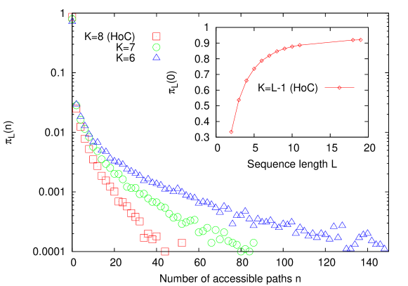
Figure 3: (Color online) Numerical study of the full distribution $\pi_{L}(n)$ of accessible paths for $L=9$ and $K=8,7,6$. Note that while for $n\geq 1$, the curves show a roughly exponential decay (linear in the logarithmic scales used here), $n=0$ carries much more weight than expected by extrapolation of the exponential. The inset shows how the corresponding probability $\pi_{L}(0)$ behaves as a function of $L$ for the HoC model ($K=L-1$). Unless indicated otherwise, the data shown in this and subsequent figures is an average over $10^{5}$ realizations

3.1 Accessible paths

Figure 3 shows an example of the distribution of the number of accessible paths, $\pi_{L}(n)$, for a fixed sequence length $L=9$ and various values of $K$. One sees that the distribution decays roughly exponentially for large values of $n$ but has much probability weight on configurations with no accessible paths at all. This implies that considering the expected number of accessible paths $\langle n_{L}\rangle$ does not suffice to characterize the distribution and one needs also to study the probability $\pi_{L}(0)$ that in a given FL, there are no accessible paths at all ch2009 ; fkdk2011 . An example for the behavior of this probability as a function of $L$ can be seen in the inset of fig. 3.

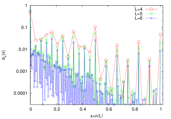
Figure 4: (Color online) Distribution of accessible paths for $K=1$ and several values of $L$ as a function of $n/L!$. This scale was chosen in order to facilitate comparison between different values of $L$. Note that the distribution is dominated by peaks that seem to persist as $L$ increases, with major peaks occurring at the same value of $x=n/L!$. In the data for $L=6$, only every third point is shown. This has no influence on the structure and only serves to render the plot less obfuscated

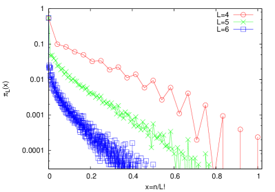
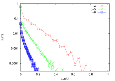
Figure 5: (Color online) $\pi_{L}(n)$ as function of $n/L!$ for $K=2$ (left) and $K=3$ (right) and different values of $L$. While the individual peaks are still discernible for small values of $L$, they become less pronounced as $L$ grows

3.1.1 Full distribution for fixed $K$: Combinatorial structure

We now consider in more detail how the shape of the distribution $\pi_{L}(n)$ changes with $K$. For $K=0$, the distribution of accessible paths is clearly given by $\pi_{L,K=0}(n)=\delta_{n,L!}$ since all paths are necessarily accessible. For $K=1$, a pronounced peak at $n=L!$ is still present, but the distribution is already dominated by realizations with no accessible paths, see fig. 4. For $K=2$, the peak structure is still present for $L=4$ but as $L$ increases, $\pi_{L}(n)$ becomes smoother, see left panel of fig 5. This can be seen even more clearly for $K=3$, where the curve for $L=6$ shows no peak structure at all anymore.

The case $K=1$ seems to play a special role in this context, as the peaks remain at the same positions (relative to the total number $L!$ of possible paths) and the peak structure is visible for all sequence lengths for which the numerical simulations were performed. Moreover, closer inspection of the distribution reveals that certain values of the number of accessible paths $n$ are forbidden, in the sense that for these values $\pi_{L}(n)=0$. In particular, the peak at $n=L!$ is separated from the rest of the distribution by a gap $\Delta n$ which increases with increasing $L$.

While the intriguing combinatorial structure seen in $\pi_{L}(n)$ for $K=1$ so far eludes our analytic understanding, the computation of $\Delta n$ is rather straightforward, as it does not depend on the details of the $LK$-model. To see this, we consider a fitness landscape in which all $L!$ paths are accessible, and ask for the minimal number of pathways that become inaccessible by reversing the fitness difference along a single nearest-neighbor bond. The number of paths passing through a bond connecting genotypes at HD $k$ and $k+1$ from the GM is $k!(L-k-1)!$, which becomes minimal at $k=\lfloor L/2\rfloor$, thus $\Delta n=\lfloor L/2\rfloor!(L-\lfloor L/2\rfloor-1)!$. This gap is present for any value of $K$, but it is relevant only for $K=1$, where the fully accessible state $n=L!$ still occurs with observable probability.

3.1.2 Expected number of accessible paths

Despite the complexity of the distribution of accessible paths, some simple analytic results are available for the expected value $\langle n_{L}\rangle$ fkdk2011 ; KlozerDiplom ; fwk2010 . Note first that, by linearity of the expectation,

$$\langle n_{L}\rangle=\sum_{k=1}^{L!}\mathbb{P}[\mathrm{path\ }k\mathrm{\ accessible}]=L!\mathbb{P}[\mathrm{path\ }k\mathrm{\ accessible}]\equiv L!P_{L}$$ (4)

where $P_{L}$ is the probability for a given path to be accessible (all paths are equivalent if one averages over realizations of the FL). For the HoC model, $P_{L}$ is the probability that $L$ i.i.d. RV’s (the fitness values encountered along the path) occur in increasing order. There is only one such ordering among the $L!$ possible permutations, and thus in the HoC case $P_{L}=1/L!$ and $\langle n_{L}\rangle=1$ independent of $L$. In the case of the RMF model (2) it can be shown that $P_{L}$ decreases exponentially (rather than factorially) with $L$ for $c>0$, implying that the expected number of accessible paths grows without bounds fwk2010 . Thus with respect to an external field, there is a clear distinction between the maximally rugged case of field strength $c=0$ and any positive field.

A similar distinction is observed numerically between the $L$-dependence of $\langle n_{L}\rangle$ when $L-K$ is kept fixed and the other two scalings, as can be seen in fig. 6. In this plot, the expected number of paths is depicted as a function of $K$ for various values of $L$. The last point for each value of $L$ corresponds to $K=L-1$. These points all lie on the line $\langle n_{L}\rangle=1$, confirming the HoC result. The second to last points correspond to $L-K=2$ and so on. While the data for $L-K\geq 2$ do not lie strictly on a line of constant $\langle n_{L}\rangle$, they increase very slowly with $K$. On the other hand, data points belonging to a fixed value of $K$ are almost equidistant along the ordinate in the semi-logarithmic plot, implying exponential growth. Similarly, if the ratio $L/K$ is kept fixed (for example at $L/K=2$ or $L/K=3$, see inset of fig. 6) a roughly exponential or slightly super-exponential growth of $\langle n_{L}\rangle$ with $L$ is observed.

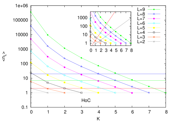
Figure 6: (Color online) Expected number of accessible paths as function of $K$ for various values of $L$. The horizontal lines indicate that for $L-K=2$, $3$ and $4$, respectively, $\langle n_{L}\rangle$ is almost constant, similar to the HoC case ($L-K=1$) where $\langle n_{L}\rangle=1$ exactly. In the inset, the points for $L/K=2$ (lower line) and $L/K=3$ (upper line) are connected by functions of the form $0.3e^{\beta K}$ with $\beta=1$ for the lower and $\beta=2$ for the upper line. This indicates that the average number of accessible paths grows exponentially with $L$ when $L/K$ is kept fixed

3.1.3 Probability of finding no accessible path

As was mentioned above in connection with the first numerical example of $\pi_{L}(n)$ in fig. 3, in addition to the expected number of accessible paths it is useful to consider also the probability $\pi_{L}(0)$ that there is no accessible path. The complementary probability $1-\pi_{L}(0)$ is the probability that there is at least one accessible path to the global fitness maximum, which can be viewed as an overall measure of accessibility ch2009 ; fkdk2011 .

For the RMF model defined in eq. (2), numerical simulations show that (similar to the expected number of accessible paths) the cases $c=0$ and $c>0$ behave very differently for large $L$ fkdk2011 . In particular, for $c>0$, $\pi_{L}(0)$ is a non-monotonic function of $L$ which declines for large $L$, indicating increasing accessibility, while for the HoC case $c=0$, $\pi_{L}(0)$ increases monotonically with $L$ and appears to approach the limit $\lim_{L\to\infty}\pi_{L}(0)=1$.

The left panel of fig. 7 shows the behavior of $\pi_{L}(0)$ for the $LK$-model at fixed values of $L-K$. The curves increase monotonically in a very similar fashion. The curve for $K=L-1$ represents the HoC case which was studied in more detail in fkdk2011 , where simulations showed that it remains monotonic at least up to $L=20$. The right panel of fig. 7 shows the behavior of $\pi_{L}(0)$ if the fraction of interaction partners $K/L$ is kept fixed. These curves show non-monotonic behavior with an increase up to a certain value of $L$ and a subsequent decrease. Thus the simulations indicate that for large $L$, there will with high probability (possibly with probability $1$) be accessible paths in such a FL.

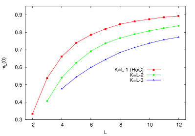
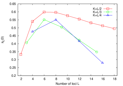
Figure 7: (Color online) Left: The probability $\pi_{L}(0)$ of no accessible path as a function of $L$, keeping $L-K$ fixed. The curve $K=L-1$ corresponds to the HoC case. All three curves increase for the entire range of $L$-values explored (up to $L=20$ for the HoC case, not shown here). Right: $\pi_{L}(0)$ at fixed ratio $K/L$

The results shown so far suggest a relatively simple picture, which matches that found previously for the RMF model fkdk2011 . Increasing $L$ at fixed $L-K$ one observes HoC-like behavior, with accessibility (measured by $1-\pi_{L}(0)$) decreasing monotonically with $L$. On the other hand, when the fraction of interacting sites is kept fixed, accessibility increases with $L$, and decreases (for large enough $L$) with increasing $K/L$, indicating that the parameter $K/L$ plays a role similar to the field $c$ in the RMF model.

However, the data depicted in fig. 8 for the behavior of $\pi_{L}(0)$ at fixed $K$ reveal a more complex scenario. The results for $K\geq 5$, which were already reported in fkdk2011 , show that, as expected, $\pi_{L}(0)$ decreases monotonically with $L$, a behavior that is seen to extend also to $K=4$ and $K=3$. In striking contrast, the curve for $K=2$ seems to be almost independent of $L$, and even more surprisingly, for $K=1$ $\pi_{L}(0)$ increases with $L$. This non-monotonic $K$-dependence of the accessibility measure $1-\pi_{L}(0)$ is highly unexpected and cannot be inferred, e.g., from the results for the expected number of accessible paths. Together with the characteristic differences in the shape of the distribution $\pi_{L}(n)$ (see above) and the corresponding distribution of basin sizes (see below), the results shown in fig. 8 provide a strong indication for a qualitative change in the $LK$ fitness landscapes at $K=2$. We will return to the possible reasons for this puzzling behavior below in sect. 4.

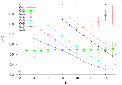
Figure 8: The probability $\pi_{L}(0)$ that a given realization of a FL has no accessible paths at all as function of the sequence length. Note that while the curves for $K\geq 3$ decrease with $L$, the curve for $K=1$ actually increases for the range of $L$ considered here. The error bars are due to a lower number of samples for larger systems ($10^{3}$ or $10^{4}$)

3.2 Basin of attraction of the global maximum

Under greedy dynamics, the configuration space can be decomposed into disjoint BoA’s, each belonging to one specific local optimum. Thus the expected size of a typical BoA, $\langle b_{typ}\rangle$, can be estimated by dividing the total number of states by the expected number of optima $\langle N_{opt}\rangle$ w1991 . For the HoC model, the average number of local optima can easily be computed: Since a local optimum has to have a greater fitness than each of its $L$ neighbors [which happens with probability $1/(L+1)$], the expected number of local optima is $\langle N_{opt}\rangle=2^{L}/(L+1)$ and hence

$$\langle b_{typ}\rangle=\frac{2^{L}}{\langle N_{opt}\rangle}=L+1.$$ (5)

Since asymptotic results for the number of local maxima in the $LK$ model exist w1991 ; es2002 ; dl2003 ; lp2004 , one can straightforwardly obtain analogous estimates for $\langle b_{typ}\rangle$ in this case. However, this only gives a lower bound to the size of $\langle b_{GM}\rangle$ of the BoA of the GM which grossly underestimates the actual behavior and will not be presented here.

One reason for the difference in behavior between $\langle b_{typ}\rangle$ and $\langle b_{GM}\rangle$ is that a typical, i.e. only local maximum has to compete for each of its nearest neighbor states with another local optimum, whereas the GM does not have to compete for its nearest neighbors: By definition, for each neighboring sequence the GM is the state of highest fitness in its neighborhood. Thus the BoA of the GM comprises at least $L+1$ configurations, whereas the BoA’s of typical maxima can be (and often are) smaller, see fig. 1 for illustration. Numerical simulations of the distribution $p_{L}(b_{GM}$ of the BoA for the HoC model show that as $L$ grows, this distribution becomes more concentrated around the minimal value $L+1$, see fig. 9. Since the HoC model is maximally rugged, the question remains whether the BoA of the GM comprises a finite fraction of the entire state space for the $LK$-model with $K<L-1$. Before addressing this question, the full size distribution of the BoA of the GM will be studied.

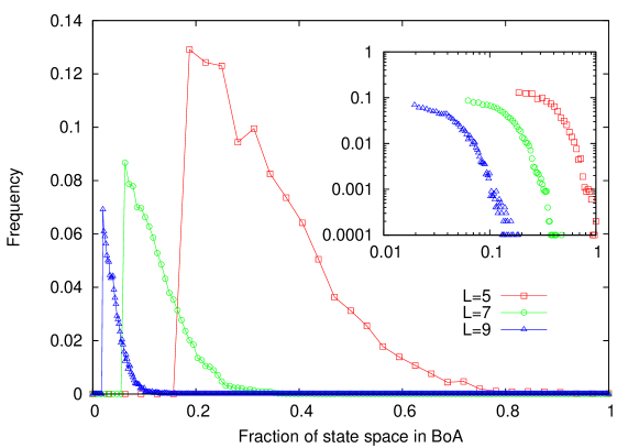
Figure 9: (Color online) Distribution of the size of the basin of attraction of the GM for the HoC model as function of the rescaled basin size $b/2^{L}$. As the sequence length $L$ increases, the distribution becomes more concentrated near the minimum value $b_{min}=L+1$. Inset shows the same data in double-logarithmic scales

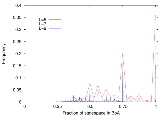
Figure 10: (Color online) Size distribution of the GM’s BoA for $K=1$ and different values of $L$ as function of the fraction of state space $b/2^{L}$. Note that the spikes dominating the distribution remain visible and occur at the same fraction of $b/2^{L}$ for all values of sequence length considered

For $K=1$, the distribution of the GM’s BoA shows a striking discrete structure with spikes that remain at fixed values of $b/2^{L}$ as $L$ grows. As can be seen in fig. 10, the most important contribution comes from realizations in which the entire state space is in the BoA, followed by contributions from realizations with exactly $3/4$ of the state space in the BoA. Similar to the distribution of the number of accessible paths for $K=1$ shown in fig. 4, the fact that the positions of dominant peaks remain at the same fraction of state space indicates that the effect causing these ‘spectra’ is commensurate (in some sense) with the total size of sequence space. Some amount of discrete structure remains visible for $K=2$ and $3$, but as can be seen in fig. 11, this appears to be a finite-size effect which becomes less prononouced as $L$ increases.

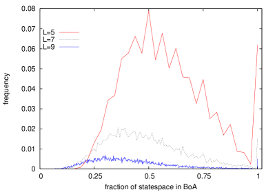
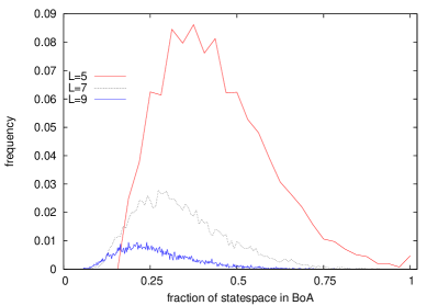
Figure 11: (Color online) Size distribution of the BoA of the GM for $K=2$ (left) and $K=3$ (right) for various sequence lengths as function of the fraction of sequence space. Note that unlike the case $K=1$, here the discrete structures vanishes as $L$ grows

Figure 12 shows in the left panel the expected size of the GM’s BoA $\langle b_{GM}\rangle$ as a function of the sequence length $L$. Clearly $\langle b_{GM}\rangle$ grows exponentially, $\langle b_{GM}\rangle\propto\exp(\alpha L)$ with $\ln 2>\alpha>0.5$ depending on $K$ (right panel of fig. 12). Since $\alpha<\ln 2$ the fraction of state space in the BoA of the GM appears to approach zero asymptotically. Similar to the results for the number of accessible paths shown in fig. 6, we see that $\langle b_{GM}(L)\rangle$ grows very slowly with $L$ when $L$ is increased at fixed $L-K$.

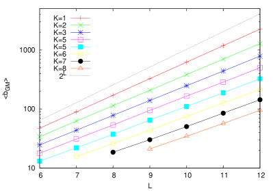
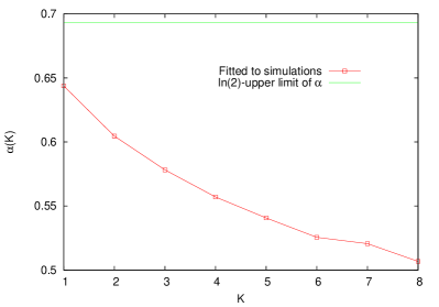
Figure 12: (Color online) The left panel shows expected size of the BoA of the GM as a function of $L$ for various values of $K$ on semi-logarithmic scales. The growth with $L$ is exponential, as indicated by the straight lines. For comparison the full volume of state space $2^{L}$ is also shown. The right panel shows the exponential growth rate $\alpha$ of the expected BoA size as function of $K$

4 Conclusions

In this paper, we investigated the evolutionary accessibility of fitness landscapes derived from Kauffman’s $LK$ model. Accessibility of these landscapes was quantified in terms of topographic properties that govern the adaptation in the strong selection/weak mutation regime (accessible paths) and the greedy regime of adaptation (basins of attraction). The $LK$ model allows to tune the number of interactions between genetic loci and thus the ruggedness of the landscape. However, it is not a priori clear how this parameter $K$, which governs the interaction strength, should behave as function of sequence length $L$. Therefore three different scalings of $K$ with $L$ were considered.

In the case of fixed difference $L-K=const.$, the accessible paths were found to behave quite similar to the totally rugged case $K=L-1$ for large $L$. However if the fraction $K/L$ is kept fixed, the landscapes become smoother in the large $L$ limit in the sense that the expected number of accessible paths grows (possibly even super-exponentially, see fig. 6) and that the probability of finding a realization without any accessible paths decays, see the right panel of fig. 7.

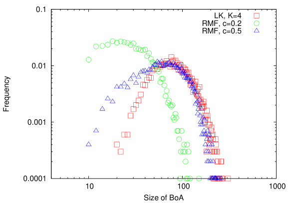
Figure 13: (Color online) Distribution of the GM’s BoA for the RMF and $LK$-models with $L=9$ and different values of $c$ and $K$ as indicated. The value $c=0.5$ for the RMF model has been chosen to match the distribution of basin sizes as obtained from the $LK$ model. Such a match is clearly not possible for $K=1$ and $2$, see figs. 10 and 11. Decreasing $c$ to the value 0.2 moves the RMF distribution close to the HoC distribution shown in the inset of fig. 9

In the case of fixed $K$, the behavior of the mean number of accessible paths $\langle n_{L}\rangle$ was found to be in accordance with the naive expectation that the resulting FL should be very smooth since $K/L\to 0$ as $L\to\infty$, see fig. 6. However the probability of no accessible paths $\pi_{L}(0)$ showed a surprising behavior. For $K\geq 3$, $\pi_{L}(0)$ declines monotonically with $L$ and the curves are very similar. For $K=1$, however, $\pi_{L}(0)$ increases with $L$. In the case $K=2$, $\pi_{L}(0)$ seems almost independent of $L$, thus this appears to be a marginal case separating the two regimes. This was not expected because $K=1$ is the (non-trivial) case with the least amount of interactions and was thus expected to be smoother than those for larger $K$.

This difference in behavior of $K=1$ and $K\geq 3$ is also reflected in the full distribution $\pi_{L}(n)$ shown in figs. 4 and 5. In one case, $\pi_{L}(n)$ remains dominated by characteristic peaks whereas for $K\geq 3$, the curves become smoother with increasing sequence length eventually showing the behavior found in fig. 3 for the HoC case $K=L-1$.

The full distribution of the BoA of the GM under greedy dynamics also showed a characteristic spike structure for $K=1$, see fig. 10. As for the distribution of the number of accessible paths, the structure remained essentially unchanged for the sequence lengths considered. Under rescaled variables $b/2^{L}$, the dominant spikes retain their positions, which indicates that the reason for these dominant features of the distribution is commensurate with the total number of states $2^{L}$.

At this point we can only speculate about the reasons for the marked change in behavior that seems to occur in the $LK$ model around $K=2$. We have noted above that the $LK$-model can be seen as a dilute spin glass with $p$-spin couplings up to $p=K+1$. In the SG context it is well known that $p$-spin models behave qualitatively different for $p=2$ and $p\geq 3$, respectively, with regard to static Gross1984 as well as dynamic Kirkpatrick1987 ; Bovier2008 properties. It remains to be seen if the observations reported here can be understood from the SG perspective.

The RMF model, which was briefly alluded to here, is another model which yields tunably rugged fitness landscapes. However, unlike the $LK$ model, the distributions obtained for the RMF model show no signs of discrete structures and, as $c\to 0$, the curves change smoothly into those from the HoC model, see for example fig. 13 and results presented in fkdk2011 . From a fitness landscape point of view it is remarkable that the way in which ‘intermediate ruggedness’ arises (by an external ‘field’ or by internal interactions) plays such an important role, while from a spin glass point of view, it is perhaps surprising that the two ways of generating intermediate ruggedness yield similar behavior at all.

Acknowledgments.

We would like to thank Johannes Berg, Anton Bovier, Bernard Derrida and Remi Monasson for useful discussions and remarks, and Alexander Klözer for his contributions in the initial stages of this project. This work was supported by DFG within SFB 680 and BCGS. JF acknowledges financial support from Studienstiftung des deutschen Volkes.

References

- (1) Darwin, C.: On the origin of species by means of natural selection, John Murray, London (1859)
- (2) Haldane, J.B.S.: The Causes of Evolution. Longmans Green & Co., London (1932)
- (3) Wright, S.: Evolution in Mendelian populations. Genetics 16, 97-159 (1931)
- (4) Fisher, R.A.: The Genetical Theory of Natural Selection. Clarendon Press, Oxford (1930)
- (5) Huxley, J.S.: Evolution: The modern synthesis, MIT Press 2010
- (6) Stemmer, W.P.C.: Rapid evolution of a protein in vitro by DNA shuffling. Nature 370, 389-391 (1994)
- (7) Weinreich, D. M., Watson, R. A., Chao, L.: Perspective: Sign epistasis and genetic constraint of evolutionary trajectories. Evolution 59, 1165-1174 (2005)
- (8) Weinreich, D.M., Delaney, N.F., DePristo, M.A., Hartl, D.L.: Darwinian evolution can follow only very few mutational paths to fitter proteins. Science 312, 111-114 (2006)
- (9) Carneiro, M., Hartl, D.L.: Adaptive landscapes and protein evolution. Proc. Natl. Acad. Sci. USA 107, 1747-1751 (2010)
- (10) Franke, J., Klözer, A., de Visser, J.A.G.M., Krug. J.: Evolutionary accessibility of mutational pathways. PLoS Comput. Biol. 7, e1002134 (2011)
- (11) Alberts, B., Johnson, A., Lewis, J., Raff, M., Roberts, K., Walter, P.: Molecular Biology of The Cell. ed., Garland Science, Taylor & Francis Group, New York (2008)
- (12) Gillespie, J.H.: Population Genetics: A Concise Guide. ed., Johns Hopkins University Press, Baltimore (2004)
- (13) Blythe, R.A., McKane, A.J.: Stochastic models of evolution in genetics, ecology and linguistics. J. Stat. Mech.: Theory Exp. P07018 (2007)
- (14) Park, S.-C., Simon, D., Krug, J.: The speed of evolution in large asexual populations. J. Stat. Phys. 138, 381-410 (2010)
- (15) Gillespie, J.H.: A simple stochastic gene substitution model. Theoretical Population Biology 23, 202-215 (1983)
- (16) Gillespie, J.H.: The Causes of Molecular Evolution. Oxford Series in Ecology and Evolution, Oxford University Press, Oxford (2002)
- (17) Orr, H.A.: A minimum on the mean number of steps taken in adaptive walks. J. Theor. Biol. 220, 241-247 (2003)
- (18) Jain, K., Krug, J.: Deterministic and stochastic regimes of asexual evolution on rugged fitness landscapes. Genetics 175, 1275-1288 (2007)
- (19) Jain, K., Krug, J., Park, S.-C.: Evolutionary advantage of small populations on complex fitness landscapes. Evolution 65, 1945-1955 (2011)
- (20) Kauffman, S.A.: The Origins of Order: Self-Organization and Selection in Evolution. Oxford University Press, Oxford (1993)
- (21) Weinberger, E.: Correlated and uncorrelated fitness landscapes and how to tell the difference. Biol. Cybern. 63, 325-336 (1990)
- (22) Stadler, P.F., Happel, R.: Random field models for fitness landscapes. J. Math. Biol. 38, 435-478
- (23) de Visser, J.A.G.M., Hoekstra, R.F., van den Enden, H.: Test of interaction between genetic markers that affect fitness in Aspergillus niger. Evolution 51, 1499-1505 (1997)
- (24) de Visser, J.A.G.M., Park, S.-C., Krug, J.: Exploring the effects of sex on empirical fitness landscapes. Am. Nat. 174, S15-S30 (2009)
- (25) Stadler, B.M.R., Stadler, P.F.: Combinatorial vector fields and the valley structure of fitness landscapes. J. Math. Biol. 61, 877-898 (2010)
- (26) Gokhale, C.S., Iwasa, Y., Nowak, M.A., Traulsen, A.: The pace of evolution across fitness valleys. J. Theor. Biol. 259, 613-620 (2009)
- (27) DePristo, M.A., Hartl, D.L., Weinreich, D.M.: Mutational reversions during adaptive protein evolution. Mol. Biol. Evol. 24 1608-1610 (2007)
- (28) Stauffer D. and Aharony A.: Introduction to percolation theory. Taylor & Francis, New York (1991)
- (29) Gavrilets, S., Gravner, J.: Percolation on the fitness hypercube and the evolution of reproductive isolation. J. Theor. Biol. 184, 51-64 (1997)
- (30) Gavrilets, S.: Fitness landscapes and the Origin of Species. Monographs in Population Biology, Princeton University Press, Princeton (2004)
- (31) Mézard, M., Parisi, G., Virasoro, M.A.: Spin Glass Theory and Beyond. World Scientific Publishing, Singapore (1987)
- (32) Mézard, M., Montanari, A.: Information, Physics, and Computation. Oxford University Press, Oxford (2009)
- (33) Hartmann, A.K., Rieger, H.: Optimization Algorithms in Physics. Wiley-VCH, Berlin (2002)
- (34) Stein, D.L. (ed.): Spin Glasses and Biology. World Scientific, Singapore (1992)
- (35) Berg, J., Willmann, S., Lässig, M.: Adaptive evolution of transcription factor binding sites. BMC Evol. Biol. 4, 42 (2004)
- (36) Sella, G., Hirsh, A.E.: The application of statistical physics to evolutionary biology. Proc. Natl. Acad. Sci. USA 102, 9541-9546 (2005)
- (37) Chou, H.-H., Chiu, H.-C., Delaney, N.F., Segrè, D., Marx, C.J.: Diminishing returns epistasis among beneficial mutations decelerates adaptation. Science 332, 1190-1192 (2011)
- (38) Khan, A.I., Dinh, D.M., Schneider, D., Lenski. R.E., Cooper, T.F.: Negative epistasis between beneficial mutations in an evolving bacterial population. Science 332, 1193-1196 (2011)
- (39) Tan, L., Serene, S., Chao, H.X., Gore, J.: Hidden randomness between fitness landscapes limits reverse evolution. Phys. Rev. Lett. 106, 198102 (2011)
- (40) Szendro, I.G., Schenk, M.F., Franke, J., Krug, J., de Visser, J.A.G.M.: Quantitative analyses of empirical fitness landscapes. arXiv:1202:4378, to appear in J. Stat. Mech.: Theor. Exp.
- (41) Kingman, J.: A simple model for the balance between selection and mutation. J. Appl. Probab. 15, 1-12 (1978)
- (42) Kauffman, S., Levin, S.: Towards a general theory of adaptive walks on rugged landscapes. J. Theor. Biol. 128, 11-45 (1987)
- (43) Derrida, B.: Random-energy model: Limit of a family of disordered models. Phys. Rev. Lett. 45, 79-82 (1980)
- (44) Derrida, B.: Random-energy model: Limit of a family of disordered systems. Phys. Rev. B 24, 2613-2626 (1981)
- (45) Miller, C.R., Joyce, P., Wichmann, H.A.: Mutational effects and population dynamics during viral adaptation challenge current models. Genetics 187, 185-202 (2011)
- (46) Aita, T. et al.: Analysis of a local fitness landscape with a model of the rough Mt.-Fuji-type landscape: Application to prolyl endepeptidase and thermolysin. Biopolymers 54, 64-79 (2000)
- (47) Kauffman, S.A., Weinberger, E.D.: The NK model of rugged fitness landscapes and its application to maturation of the immune response. J. Theor. Biol. 141, 211-245 (1989)
- (48) de Visser, J.A.G.M., Cooper, T.F., Elena, S.F.: The causes of epistasis. Proc. R. Soc. Lond. B 278, 3617-3624 (2011)
- (49) Fontana, W. et al.: RNA folding and combinatory landscapes. Phys. Rev. E 47, 2083-2099 (1993)
- (50) Perelson, A.S., Macken, C.A.: Protein evolution on partially correlated landscapes. Proc. Natl. Acad. Sci. USA 92, 9657-9661 (1995)
- (51) Welch, J.J., Waxman, D.: The nk model and population genetics. J. Theor. Biol. 234, 329-340 (2005)
- (52) Weinberger, E.D.: Fourier and Taylor series on fitness landscapes. Biol. Cybern. 65, 321-330 (1991)
- (53) Neher, R.A., Shraiman, B.I.: Statistical genetics and evolution of quantitative traits. Rev. Mod. Phys. 83, 1283-1300 (2011)
- (54) Drossel, B.: Biological evolution and statistical physics. Adv. Phys. 50, 209-295 (2001)
- (55) Derrida, B., Gardner, E.: Metastable states of a spin glass chain at 0 temperature. J. Physique 47, 959-965 (1986)
- (56) Weinberger, E.D.: Local properties of Kauffman’s model: A tunably rugged energy landscape. Phys. Rev. A 44, 6399-6413 (1991)
- (57) Evans, S.N., Steinsaltz, D.: Estimating some features of fitness landscapes. Annals of Probability 12, 1299-1321 (2002)
- (58) Durrett, R., Limic, V.: Rigorous results for the model. Annals of Probability 31, 1713-1753 (2003)
- (59) Limic, V., Pemantle, R.: More rigorous results on the Kauffman-Levin model of evolution. Annals of Probability 32, 2149-2187 (2004)
- (60) Østman, B., Hintze, A., Adami, C: Impact of epistasis and pleiotropy on evolutionary adaptation. Proc. R. Soc. B 279, 247-256 (2012)
- (61) Klözer, A.: Fitness Landscapes. Diploma Thesis, Universität zu Köln, 2008
- (62) Franke J., Wergen G. and Krug J.: Records and sequences of records from random variables with a linear trend. J. Stat. Mech.: Theor. Exp., P10013 (2010)
- (63) Gross, D.J., Mézard, M.: The simplest spin glass. Nucl. Phys. B 240, 431-452 (1984)
- (64) Kirkpatrick, T.R., Thirumalai, D.: Dynamics of the structural glass transition and the -spin-interaction spin-glass model. Phys. Rev. Lett. 58, 2091-2094 (1987)
- (65) Ben Arous, G., Bovier, A., Černý, J.: Universality of random energy model-like ageing in mean field spin glasses. J. Stat. Mech. L04003 (2008)