$J$-state interference signatures in the Second Solar Spectrum

The scattering polarization in the solar spectrum is traditionally modeled with each spectral line treated separately, but this is generally inadequate for multiplets where $J$-state interference plays a significant role. Through simultaneous observations of all the 3 lines of a Cr i triplet, combined with realistic radiative transfer modeling of the data, we show that it is necessary to include $J$-state interference consistently when modeling lines with partially interacting fine structure components. Polarized line formation theory that includes $J$-state interference effects together with partial frequency redistribution for a two-term atom is used to model the observations. Collisional frequency redistribution is also accounted for. We show that the resonance polarization in the Cr i triplet is strongly affected by the partial frequency redistribution effects in the line core and near wing peaks. The Cr i triplet is quite sensitive to the temperature structure of the photospheric layers. Our complete frequency redistribution calculations in semi-empirical models of the solar atmosphere cannot reproduce the observed near wing polarization or the cross-over of the Stokes $Q/I$ line polarization about the continuum polarization level that is due to the $J$-state interference. When however partial frequency redistribution is included, a good fit to these features can be achieved. Further, to obtain a good fit to the far wings, a small temperature enhancement of the FALF model in the photospheric layers is necessary.

1 Introduction

The Second Solar Spectrum is produced by coherent scattering processes in the solar atmosphere (Stenflo 1994). Modeling this spectrum requires the solution of the polarized radiative transfer (RT) equation. It is well known that quantum interference between the fine structure ($J$) levels is responsible for the formation of line pairs such as Na i D₁ and D₂, Ca ii H and K, etc. The linear polarization in the Ca ii H and K lines was observed and modeled by Stenflo (1980), who developed a theoretical framework which for the first time demonstrated the profound role that quantum interference between different fine structure components within a multiplet can have on the observed polarization profiles. An extended version of this theoretical framework, applicable to any multiplet, was presented in Stenflo (1997). It was used for RT modeling of $J$-state interference in the Na i D₁ and D₂ lines by Fluri et al. (2003). The $J$-state interference theory used in the mentioned papers assumed frequency coherent scattering. Recently Smitha et al. (2011a, hereafter P1) have extended the theory of Stenflo (1997) to include partial frequency redistribution (PRD) with $J$-state interference. It is restricted to the case of a two-term atom and uses the assumption that the lower term is unpolarized. Landi Degl’Innocenti et al. (1997) have proposed an alternative approach to the same problem based on the concept of metalevels, which is intended for dealing with PRD in multi-term atoms. A multi-term formulation of $J$-state interference that accounts for the polarization in all the terms, but which is restricted to the case of complete frequency redistribution (CRD), has been given in Landi Degl’Innocenti & Landolfi (2004, hereafter LL04). In the mentioned theoretical formulations collisional frequency redistribution was not included.

In Smitha et al. (2011b, hereafter P2) the redistribution matrix for the $J$-state interference derived in P1 was incorporated into the RT equation, which was solved for simple isothermal model atmospheres. Several theoretical aspects of radiative transfer in a hypothetical doublet line system are studied in that paper. The purpose of the present paper is to perform one-dimensional RT modeling of the polarimetric observations of a multiplet where $J$-state interference is relevant. For this we have selected the Cr i triplet at 5204.50 Å (line-1: $J_{b}=1\to J_{a}=2$), 5206.04 Å (line-2: $J_{b}=2\to J_{a}=2$), and 5208.42 Å (line-3: $J_{b}=3\to J_{a}=2$). Hyperfine splitting can be neglected because the most abundant (90%) isotope of Cr i has zero nuclear spin.

Kleint et al. (2010a,b) have used the Cr i triplet for a synoptic program to explore solar cycle variations of the microturbulent field strength. Recently, Belluzzi & Trujillo Bueno (2011) applied the density matrix theory described in LL04 (which is based on the CRD approximation) in order to perform a basic investigation on the impact of $J$-state interference in several important multiplets in the solar spectrum including also the Cr i triplet. In this work they have neglected RT and PRD effects. However, they have included the effects of lower term polarization and the dichroism. They identify and explain qualitatively the observational signatures produced by $J$-state interference in the Cr i triplet (i.e., the cross-over of $Q/I$ about the continuum polarization level occurring between the lines, and the $Q/I$ feature around the line-1 core).

In Section 2 we briefly present the basic equations required for realistic RT modeling of lines in the two-term atom picture. In Section 3 we present the polarimetric observations of the Cr i triplet. Section 4 is devoted to a description of realistic modeling of the observations. In Section 5 we present the main results. Concluding remarks are given in Section 6.

2 Polarized line transfer equation for a two-term atom

In a non-magnetic medium, the polarization of the radiation field is represented by the Stokes vector $(I,Q)^{\rm T}$, where positive $Q$ is defined to represent linear polarization that is oriented parallel to the solar limb. In a medium that is axisymmetric around the vertical direction, it is advantageous to use a formulation in terms of the reduced Stokes vector ${\bm{\mathcal{I}}}$ instead of the traditional Stokes vector $(I,Q)^{\rm T}$. The transformations between the two can be found in Appendix B of Frisch (2007). The relevant line transfer equation for the 2-component reduced Stokes vector is

$$\mu\frac{{\partial{\bm{\mathcal{I}}}(\lambda,\mu,z)}}{\partial z}=-k_{\rm tot}(\lambda,z)\left[{\bm{\mathcal{I}}}(\lambda,\mu,z)-{\bm{\mathcal{S}}}(\lambda,z)\right],$$ (1)

in standard notation (see Anusha et al. 2011). $z$ is the geometric height in the atmosphere. See P2 for details of Eq. (1) and related quantities. The total opacity $k_{\rm tot}(\lambda,z)=\eta_{M}(\lambda,z)+\sigma_{c}(\lambda,z)+k_{c}(\lambda,z)$, where $\sigma_{c}$ and $k_{c}$ are the continuum scattering and continuum absorption coefficients, respectively. The line absorption coefficient for the entire multiplet is

$$\eta_{M}(\lambda,z)\! = \!k_{M}(z)\phi_{M}(\lambda,z)=\!\!\sum_{J_{a}J_{b}}k_{l(J_{b}J_{a})}\phi(\lambda_{J_{b}J_{a}},z),$$ (2)

where $k_{l(J_{b}J_{a})}$ is the wavelength averaged absorption coefficient for the $J_{a}\to J_{b}$ transition with the corresponding profile function denoted by $\phi(\lambda_{J_{b}J_{a}},z)$. $J_{b}$ and $J_{a}$ are the total angular momentum quantum numbers of the fine-structure levels for the upper and lower terms (see Fig. 1). $k_{M}(z)$ is the wavelength averaged absorption coefficient for the entire multiplet. For our case of a two-term atom, we need to define a combined profile function that determines the shape of the absorption coefficient across the whole multiplet. It can be shown that for the Cr i triplet line system $\phi_{M}(\lambda,z)$ is given by (see Eqs. (7) and (8) in Section 2 of P2)

$$\phi_{M}(\lambda,z)=\frac{3\phi(\lambda_{1\,2},z)+5\phi(\lambda_{2\,2},z)+7\phi(\lambda_{3\,2},z)}{15}.$$ (3)

The reduced source vector is defined as

$$\bm{\mathcal{S}}(\lambda,z) = \frac{k_{M}(z)\phi_{M}(\lambda,z)\bm{\mathcal{S}}_{l}(\lambda,z)+\sigma_{c}(\lambda,z)\bm{\mathcal{S}}_{c}(\lambda,z)}{k_{\rm tot}(\lambda,z)}$$ (4)

$$+\frac{k_{c}(\lambda,z)\bm{\mathcal{S}}_{\rm th}(\lambda,z)}{k_{\rm tot}(\lambda,z)},$$

for a two-term atom with an unpolarized lower term. Here $\bm{\mathcal{S}}_{\rm th}=(B_{\lambda},0)^{T}$, where $B_{\lambda}$ is the Planck function. The continuum scattering source vector is

$${\bm{\mathcal{S}}}_{c}(\lambda,z)=\frac{1}{2}\int_{-1}^{+1}\hat{\Psi}(\mu^{\prime}){\bm{\mathcal{I}}}(\lambda,\mu^{\prime},z)\,d\mu^{\prime}.$$ (5)

Since continuum polarization can be seen as representing scattering in the distant wings of spectral lines (in particular from the Lyman series lines, cf. Stenflo 2005), we are justified to use the assumption of frequency coherent scattering for the continuum. The matrix $\hat{\Psi}$ is the Rayleigh scattering phase matrix in the reduced basis (see Frisch 2007). The line source vector

$${\bm{\mathcal{S}}}_{l}(\lambda,z) = \epsilon\bm{\mathcal{S}}_{\rm th}(\lambda,z)+\int_{-\infty}^{+\infty}\frac{1}{2}$$ (6)

$$\ \ \ \ \ \ \ \times\int_{-1}^{+1}\frac{\widetilde{{\bm{\mathcal{R}}}}(\lambda,\lambda^{\prime},z)}{\phi_{M}(\lambda,z)}\hat{\Psi}(\mu^{\prime}){\bm{\mathcal{I}}}(\lambda^{\prime},\mu^{\prime},z)\,d\mu^{\prime}\,d\lambda^{\prime}.$$

Figure 1: The term diagram showing transitions in the Cr I triplet. The diagram is not drawn to scale.

The thermalization parameter $\epsilon={\Gamma_{I}}/(\Gamma_{R}+\Gamma_{I})$ where $\Gamma_{R}$ and $\Gamma_{I}$ are the radiative and inelastic collisional de-excitation rates, respectively. $\widetilde{{\bm{\mathcal{R}}}}(\lambda,\lambda^{\prime},z)$ is a $(2\times 2)$ diagonal matrix with elements $\widetilde{{\bm{\mathcal{R}}}}=$ diag $({\mathcal{R}}^{0},{\mathcal{R}}^{2})$, where ${\mathcal{R}}^{K}$ are the redistribution functions which include the effects of $J$-state interference between different line components in a multiplet. ${\mathcal{R}}^{K}$ represents a linear combination of redistribution functions of type-II and type-III. In the reduced Stokes vector basis, the angular phase matrix and the frequency redistribution functions are decoupled. The phase matrix part is built into the transfer equation through the $\hat{\Psi}$ matrix. The theory of redistribution matrices for the $J$-state interference in two-term atoms for the collisionless case is presented in P1. This frequency redistribution part that includes $J$-state interference and the collisional redistribution is given by

$${\bf{\mathcal{R}}}^{K}(x,x^{\prime})=\frac{3(2L_{b}+1)}{2S+1}\sum_{J_{a}J_{f}J_{b}J_{b^{\prime}}}(-1)^{J_{f}-J_{a}}$$

$$\times\langle\tilde{r}_{J_{b}}\tilde{r}^{\ast}_{J_{b^{\prime}}}\rangle_{J_{a}J_{f}}(2J_{a}+1)(2J_{f}+1)(2J_{b}+1)(2J_{b^{\prime}}+1)$$

$$\times\left\{\begin{array}[]{ccc}L_{a}&L_{b}&1\\ J_{b}&J_{f}&S\\ \end{array}\right\}\left\{\begin{array}[]{ccc}L_{a}&L_{b}&1\\ J_{b}&J_{a}&S\\ \end{array}\right\}\left\{\begin{array}[]{ccc}L_{a}&L_{b}&1\\ J_{b^{\prime}}&J_{f}&S\\ \end{array}\right\}$$ (13)

$$\times\left\{\begin{array}[]{ccc}L_{a}&L_{b}&1\\ J_{b^{\prime}}&J_{a}&S\\ \end{array}\right\}\left\{\begin{array}[]{ccc}1&1&K\\ J_{b^{\prime}}&J_{b}&J_{a}\\ \end{array}\right\}\left\{\begin{array}[]{ccc}1&1&K\\ J_{b^{\prime}}&J_{b}&J_{f}\\ \end{array}\right\}.$$ (20)

The ensemble averaged coherency matrix elements (see e.g., Bommier & Stenflo 1999) in the above equation are given by

$$\langle\tilde{r}_{J_{b}}\tilde{r}^{\ast}_{J_{b^{\prime}}}\rangle_{J_{a}J_{f}}=A\cos\beta_{J_{b^{\prime}}J_{b}}$$

$$\times[\cos\beta_{J_{b^{\prime}}J_{b}}(h^{\rm II}_{J_{b},J_{b^{\prime}}})_{J_{a}J_{f}}-\sin\beta_{J_{b^{\prime}}J_{b}}(f^{\rm II}_{J_{b},J_{b^{\prime}}})_{J_{a}J_{f}}]$$

$$+B^{(K)}\cos\beta_{J_{b^{\prime}}J_{b}}\cos\alpha^{(K)}_{J_{b^{\prime}}J_{b}}$$

$$\!\!\!\!\times\Bigg{\{}\cos\big{(}\beta_{J_{b^{\prime}}J_{b}}+\alpha^{(K)}_{J_{b^{\prime}}J_{b}}\big{)}\left[\Re\bigg{(}{h^{\rm III}_{J_{b}J_{a},J_{b^{\prime}}J_{f}}}\bigg{)}-\Im{\bigg{(}f^{\rm III}_{J_{b}J_{a},J_{b^{\prime}}J_{f}}\bigg{)}}\right]$$

$$\!\!\!\!-\sin\big{(}\beta_{J_{b^{\prime}}J_{b}}+\alpha^{(K)}_{J_{b^{\prime}}J_{b}}\big{)}\left[\Im\bigg{(}{h^{\rm III}_{J_{b}J_{a},J_{b^{\prime}}J_{f}}}\bigg{)}+\Re{\bigg{(}f^{\rm III}_{J_{b}J_{a},J_{b^{\prime}}J_{f}}\bigg{)}}\right]\Bigg{\}}.$$ (21)

The $(h^{\rm II}_{J_{b},J_{b^{\prime}}})_{J_{a}J_{f}}$ and $(f^{\rm II}_{J_{b},J_{b^{\prime}}})_{J_{a}J_{f}}$ are the auxiliary functions defined in Eqs. (14) and (15) of P1 but are used here for the non-magnetic case and with angle-averaged redistribution functions of type-II. The auxiliary functions of type-II derived in P1 represents generalizations of the corresponding quantities appearing in Sampoorna (2011, see Eqs. (22) and (23)) using a semi-classical approach. The important difference between the two in the presence of the magnetic field is that in case of $J$-state interference these auxiliary functions depend on both $J$ and $m$ quantum numbers, unlike in case of $m$-state interference where they depend only on $m$. In the particular case of non-magnetic $J$-state interference theory, these quantities depend only on $J$ quantum numbers, whereas the corresponding quantities in the $m$-state interference theory simply reduce to the well known type-II redistribution functions of Hummer (1962). Therefore for the notational brevity even in the $J$-state interference case we refer to these auxiliary functions as $R_{\rm II}$ hereafter (in the standard notation of Hummer 1962).

The auxiliary quantities for type-III redistribution (see the last two lines of Eq. (21)) in the non-magnetic case are also derived in a way similar to the two-level atom case given in Eqs. (27)-(36) of Sampoorna (2011). But in doing so the following assumptions are made

1. Infinitely sharp lower term.

2. Unpolarized lower term.

3. Weak radiation field limit (i.e., stimulated emission is neglected in comparison with spontaneous emission).

4. Hyperfine structure is neglected.

5. The (inelastic) collisions that transfer polarization between fine structure levels of a given term (upper or lower) are neglected.

6. The depolarizing elastic collisions that couple $m$-states belonging to a given fine structure level $J_{b}$ are considered and taken to be same for a given term.

7. We restrict our attention to the linear Zeeman regime (Zeeman splitting much smaller than the fine structure splitting). This is not applicable in the Paschen-Back regime.

The assumption of an unpolarized lower term is made for the sake of mathematical simplicity. The inelastic collisions that transfer polarization between the fine structure levels are neglected. This is justified because the colliding particles are isotropically distributed around the radiating atom. This situation is similar to the case of an atom immersed in an isotropic radiation field producing no atomic polarization (scattering polarization). Neglecting such inelastic collisions is particularly valid in the linear Zeeman regime in which we are interested. However these inelastic collisions do cause population transfer between the fine structure levels, and are properly accounted for in the calculations of line opacities (see Section 4).

The angle $\beta_{J_{b^{\prime}}J_{b}}$ is defined in Eq. (10) of P1. The angle $\alpha^{(K)}_{J_{b^{\prime}}J_{b}}$ is defined as

$$\tan\alpha^{(K)}_{J_{b^{\prime}}J_{b}}=\frac{\omega_{J_{b^{\prime}}J_{b}}}{\Gamma_{R}+\Gamma_{I}+D^{(K)}}.$$ (22)

Here $\hbar\omega_{J_{b^{\prime}}J_{b}}$ is the energy difference between the $J_{b^{\prime}}$ and $J_{b}$ states in the absence of a magnetic field. $D^{(K)}$ is the $2K$ multipole depolarizing elastic collisional destruction rate. In general $D^{(K)}$ depend on the $J$ quantum numbers of the fine structure states. As a simplifying assumption, we take these rates to be the same for all the fine structure states of the upper term, and use the classical value $D^{(K)}=\Gamma_{E}/2$ given by Stenflo (1994) where $\Gamma_{E}$ is the elastic collision rate which is responsible for the broadening of the atomic states. $A$ and $B^{(K)}$ are the branching ratios which are given by

$$A=\frac{\Gamma_{R}}{\Gamma_{R}+\Gamma_{I}+\Gamma_{E}};\quad B^{(K)}=\frac{\Gamma_{R}}{\Gamma_{R}+\Gamma_{I}+D^{(K)}}\frac{\Gamma_{E}-D^{(K)}}{\Gamma_{R}+\Gamma_{I}+\Gamma_{E}}.$$ (23)

These branching ratios are the ones derived for a two-level atom model by Bommier (1997). In view of the simplifying assumptions stated above, we continue to use the same branching ratios for the two-term atom case also.

The computation of angle-averaged type-III redistribution functions (that appear in Eq. (21)) is very expensive, especially for the case of a realistic model atmosphere. Therefore we prefer to use the approximation of CRD in place of type-III redistribution functions (see Mihalas 1978). We have verified by direct numerical computations that this replacement is valid and gives results which are almost identical to the explicit use of type-III redistribution functions. The necessary settings of the branching ratios in order to go to the limit of pure CRD are $A=0$ and $B^{(K)}=(1-\epsilon)$ (see also Anusha et al. 2011).

3 Observational details

The $Q/I$ spectra of Cr i triplet were observed by Gandorfer (2000). In this paper, we present new observations of this triplet obtained with the ZIMPOL-3 polarimeter (Ramelli et al. 2010) at IRSOL in Switzerland. Fig. 2 shows the observations recorded on September 6, 2011, at the heliographic north pole with the slit placed parallel to the limb at $\mu=0.15$. The polarization modulation was done with a piezo-elastic modulator (PEM). The spectrograph slit was $60\mu$m wide corresponding to a spatial extent of $0.5^{\prime\prime}$ on the solar image. The CCD covered $190^{\prime\prime}$ along the slit. The effective pixel resolution in the spatial direction is 4 actual pixels wide, due to the grouping of each four pixel rows covered by a cylindrical microlense, to allow simultaneous recording of all four Stokes parameters in the ZIMPOL demodulation scheme. The resulting CCD images have 140 such effective pixel resolution elements in the spatial direction, each element corresponding to $1.38^{\prime\prime}$, and 1240 pixels in the wavelength direction, with one pixel corresponding to 7.84 mÅ. In Fig. 2 only the central part of the spectral window, corresponding to 1050 pixels spanning 8.23 Å, is displayed. With the PEM it was possible to measure simultaneously one linear and the circular polarization component. Measurements of the linear polarization component $Q/I$ were alternated with measurements of the $U/I$ component through mechanical rotation of the analyzer by $45^{\circ}$. In total we accumulated for both the components 2000 exposures of 1 second each.

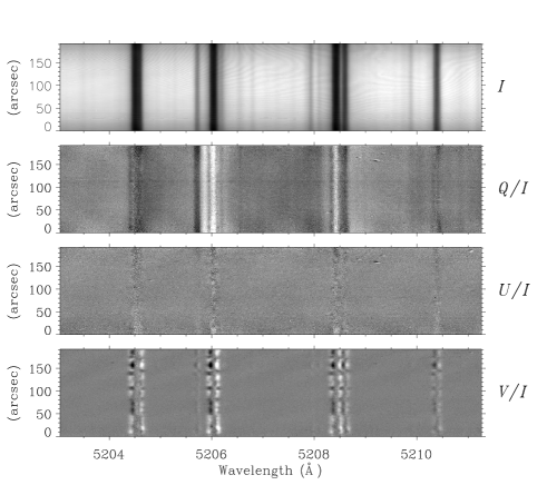
Figure 2: CCD image showing the $(I,Q/I,U/I,V/I)$ of the Cr i triplet. The recording was made on September 6, 2011, near the heliographic north pole at a limb distance defined by $\mu=0.15$. The grey scale cuts span a range (from black to white) of 0.1 % in $Q/I$ and $U/I$, while for $V/I$ the cuts are $-0.2$ % (black) and $+0.2$ % (white).

4 Modeling of Cr i triplet

To model the Cr i triplet the polarized spectrum is calculated by a two-stage process described in Holzreuter et al. (2005, see also Anusha et al. 2010, 2011). In the first-stage a multi-level PRD-capable MALI (Multi-level Approximate Lambda Iteration) code of Uitenbroek (2001, referred to as the RH-code) solves the statistical equilibrium equation and the unpolarized RT equation self-consistently and iteratively. The RH-code is used to compute the unpolarized intensities, opacities and the collision rates. The angle-averaged redistribution functions of Hummer (1962) are used in the RH-code to represent PRD in line scattering. In the second stage the opacities and the collision rates are kept fixed, and the polarized intensity vector $\bm{\mathcal{I}}$ is computed perturbatively by solving the polarized RT equation with the redistribution matrices defined in Section 2, which are derived for a two-term atom with an unpolarized lower term.

4.1 Model atom and model atmosphere

The Cr i atom model is constructed for 14 levels (13 levels of Cr i and the ground state of Cr ii), 11 line transitions, and 13 continuum transitions. The line components of the ${}^{5}\!S-^{5}\!\!P$ triplet of Cr i are considered under PRD. The values of the various physical quantities required to build the atom model are taken from the NIST atomic data base and the Kurucz data base. The data for the blend lines are also obtained from the Kurucz data base. The photo-ionization cross sections are taken from Bergemann & Cescutti (2010). The explicit dependence of these cross sections on wavelength is computed under the hydrogenic approximation.

Fig. 3a shows the temperature structure in some of the standard model atmospheres of the Sun - namely FALA, FALC, FALF (Fontenla et al. 1993), and FALX (Avrett 1995), which we have used in our attempts to fit the observed $(I,Q/I)$ spectra. Models A, C and F of Fontenla et al. (1993) represent respectively the supergranular cell center, the average quite Sun, and the bright network region in the solar atmosphere. FALX represents the coolest model with a chromospheric temperature minimum located around 1000 km above the photosphere. Our attempts to fit the observed $(I,Q/I)$ spectra using these standard models will be discussed in Sect. 5.2.

We show that a reasonable fit could be obtained only with a temperature structure modified with a small enhancement in the original temperature structure of the FALF model, in the height range of 100 km below the photosphere, extending up to 700 km above the photosphere (denoted by $\overline{\rm FALF}$). Such an enhancement does not affect the center to limb variation (CLV) of the continuum intensity as shown in Fig. 3b. While such a modification of the temperature structure produces insignificant changes in the intensity spectra, $Q/I$ turns out to be quite sensitive to these changes in the temperature gradient.

In order to explore the effect of temperature enhancement in a given model atmosphere used for computing line and continuous spectra, we have performed a simple test (similar to the Fig. 3 of Asplund et al. 1999, see our Fig. 3c). It is expected that 1D model atmospheres (like FALF in our case; or all the FAL class of models in general) fit the observed CLV data of continuum intensity to a good accuracy. To verify this, we have plotted the limb darkening function for the whole range of wavelengths, for different $\mu$ values. The theoretical limb darkening function fits the corresponding observed data better for $\mu\to 1$. The fit is approximate in the limb positions (say $\mu=0.1$). In Fig. 3c we also show the theoretical curves computed for the $\overline{\rm FALF}$ model (dotted lines). As can be seen, the limb darkening function of $\overline{\rm FALF}$ does not greatly differ from that of the original FALF model atmosphere (a maximum relative difference of 15% in the extreme limb). Therefore it justifies a slight modification of temperature structure in a given model atmosphere to achieve a theoretical fit to the $Q/I$ observations.

Figure 3: Panel (a) shows the temperature structure of several standard model atmospheres. $\overline{\rm FALF}$ represents a model with an enhanced temperature structure of the original FALF model. In panel (b) we show the center to limb variation of the ‘limb darkening function’, $I_{c}(\mu)/I_{c}(\mu=1)$, where $I_{c}(\mu)$ is the continuum intensity near the Cr i triplet. Panel (c) shows the CLV of the continuum intensity for all wavelengths covering the violet to the IR regions of the spectrum. The observed data are taken from Neckel & Labs (1994).

5 Results and discussion

5.1 Comparison between PRD and CRD

Fig. 4 shows the comparison between the $Q/I$ profiles computed using only CRD (to represent frequency non-coherent redistribution: solid line), only $R_{\rm II}$ (dotted line), and a combination of $R_{\rm II}$ and CRD (dashed line) (see Section 2 for the definition of CRD). As seen from the figure, the CRD profiles do not produce the wing peaks on either side of the line center, which are clearly seen in the PRD profiles. Also, the $J$-state interference signatures are more prominent in PRD than in CRD. A good fit to the observed $Q/I$ can only be achieved through the use of PRD (see Section 5.2). We have verified that it is impossible to fit the observed near wing peaks with CRD alone. The pure $R_{\rm II}$ mechanism represents frequency coherent scattering in the line wings, the use of which alone also fails to achieve a good fit (since it produces too large values of $Q/I$ throughout the wings). We find that a proper combination of $R_{\rm II}$ and CRD is essential to obtain a good fit to the observations. This can be seen more clearly in Fig. 7, where we present a comparison with the observed $Q/I$ profile. It is well known that only such a combination can correctly take into account the collisional frequency redistribution.

Therefore the $(R_{\rm II},$CRD$)$ combination is adopted for the computations in the present paper.

The effect of elastic collisions is to cause significant depolarization in the line wings. This can be seen from the dashed line in Fig. 4a, which shows that due to elastic collisions the line wing amplitudes of $Q/I$ are greatly suppressed with respect to the corresponding pure $R_{\rm II}$ case (dotted line). The fact that the Cr i line components are formed in the upper photosphere and lower chromosphere makes it necessary to include elastic collisions in our theoretical modeling. The issue of elastic collisions is discussed in some detail in Section 2.

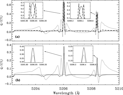
Figure 4: ($Q/I$) of the Cr i triplet computed with CRD (solid line), $R_{\rm II}$ (dotted line), and a combination of CRD and $R_{\rm II}$ (dashed line) for $\mu=0.15$. The positive $Q$ represents linear polarization parallel to the solar limb. The thin solid line in $Q/I$ at the 0.025 % level represents the continuum polarization. The microturbulent magnetic field $B_{\rm turb}=0$. No spectral smearing is applied to the profiles in the panel (a). In the line core the $Q/I$ profiles computed with pure $R_{\rm II}$ and with a combination of $R_{\rm II}$ and CRD nearly coincide (see the insets in the panel (a)). The panel (b) shows a comparison between the $Q/I$ profiles computed with CRD and with $R_{\rm II}$ when we also apply a spectral smearing of 80 mÅ. The line types have the same meanings as in panel (a).

Fig. 4b shows the effect of spectral smearing that needs to be applied to the theoretical profiles in order to compare them with the observed profiles, which are broadened by the particular spectral resolution that was used in the observations. In the absence of smearing the $Q/I$ in the line core computed with $R_{\rm II}$ and CRD differ significantly (see Fig. 4a). These differences decrease drastically after application of spectral smearing. Although in isothermal atmospheric models $Q/I$ computed with pure $R_{\rm II}$ and with CRD are very similar in the line center region, the same cannot be expected in computations with realistic atmospheres. Indeed $Q/I$ computed with PRD shows a double peak structure in the line core region with a dip at line center (see Holzreuter et al. 2005 for details). The smearing wipes out the double-peaked core structure that we see in Fig. 4a.

5.2 Comparison with observations

In this section we compare the theoretical Stokes profiles computed using several standard atmospheric models of the Sun, with the observations. Figs. 5 and 6 show the $I/I_{c}$ and $Q/I$ spectra. From Fig. 5 we can see that the $I/I_{c}$ is not sensitive to the choice of the model atmospheres, whereas $Q/I$ is very sensitive. The reason for this sensitivity is the angular anisotropy of the radiation field, which is different for different atmospheres.

Figure 5: Intensity spectra for a choice of model atmospheres. The dotted line represents observations and the solid line represents the theoretical profiles. The line of sight is represented by $\mu=0.15$.

Figure 6: The polarized ($Q/I$) spectra computed at $\mu=0.15$ and for a choice of model atmospheres. The line types are the same as in Fig. 5. The dashed line represents the level of continuum polarization. The observations are taken at $\mu=0.15$. The $B_{\rm turb}$ values used for the theoretical profiles are given in Table 1.

From Fig. 3 it is clear that the temperature structure of these models are considerably different from each other in the line formation region. We find that a modification of the temperature structure at certain range in the atmosphere does not significantly affect the emergent $I/I_{c}$ profile. However $Q/I$ is quite sensitive to such ‘modifications’ in the temperature structure in the line formation region. The theoretical profiles (solid lines) in Fig. 6 are computed taking into account the effects of microturbulent magnetic fields ($B_{\rm turb}$) with an isotropic angular distribution (Stenflo 1994). Further, the spectral smearing (see Anusha et al. 2010) is done using a Gaussian function with FWHM of 80 mÅ. The use of $B_{\rm turb}$ is essential to obtain correct line center amplitudes of $Q/I$. The values of $B_{\rm turb}$ for the three components of the Cr i triplet are different. They are chosen to fit the observed line center amplitudes of $Q/I$ using the FALF model. In this way, the microturbulent magnetic field strength is only used as a free parameter to improve the fit with the observations. We have made no attempt to achieve a good fit to the line center amplitudes of the $(Q/I)$ profile computed using FALA, FALC and FALX models. FALF provides a better fit to the observed $Q/I$ profiles at the cores of the three lines and the interference regions in between them. However the far wings still remain poorly fitted even by the FALF model. To achieve a good fit to the far wing region of all the three lines, we found it necessary to enhance (see Fig. 3) the temperature in the layers where the far wings are formed.

Figure 7: Comparison between the limb ($\mu=0.15$) observations (dotted line, representing the $Q/I$ spectrum of Fig. 2 averaged along the slit) and the theoretical profile (solid line). The centers of the 3 lines, the PRD peak positions of line-2 and line-3, and the cross-over wavelength positions between the lines are marked with vertical lines. The dashed line in $Q/I$ at 0.025 % represents the continuum polarization level. The solid line is the same as the dashed line of Fig. 4a, except that we have now introduced Hanle depolarization due to microturbulent magnetic fields (see Table 1), and added spectral smearing of 80 mÅ to simulate the observations. The smearing wipes out the double-peaked core structure that we see in Fig. 4a.

Fig. 7 shows a comparison between the profiles of the Cr i triplet computed with the $J$-state interference theory (solid line) and the observed data (dotted line). This solid line is the same as the dashed line in Fig. 4a, except that it now also includes the contributions from $B_{\rm turb}$ and a spectral smearing of 80 mÅ  to simulate the observations. The best fit values of $B_{\rm turb}$ for the 3 components of the Cr i triplet are given in Table 1. The approximate heights of formation given in Table 1 are the heights at which the condition $\tau(\lambda_{0})/\mu\simeq 1$ is satisfied for $\mu=0.15$. The quantity $\tau(\lambda_{0})$ is the total optical depth at line center for the $\overline{\rm FALF}$ model.

The observed $Q/I$ spectra of the Cr i triplet have two main characteristics, namely (i) the presence of a triple peak structure in line-2 and line-3; (ii) the cross over of $Q/I$ about the continuum polarization level, occurring between the line components. These two aspects are well reproduced in terms of the theoretical framework with the redistribution matrix theory for $J$-state interference developed in P1 and P2. The small discrepancies between the observations and theoretical profiles in $Q/I$ can be attributed to the presence of blend lines. The blend lines are assumed to be formed under LTE and generally depolarize the wings of the main line as well as the continuum polarization. To fit the observed $I$ spectra the oscillator strengths of the blend lines from the Kurucz data base are used unchanged, with the single exception of the Y ii line at 5205.75 Å, since the value from the data base for this line does not reproduce the Stokes $I$ spectrum at all. Therefore the oscillator strength for this line is changed substantially to get a good Stokes $I$ fit. As soon as the Stokes $I$ fit becomes good, the $Q/I$ fit automatically becomes good as well around 5205.75 Å. Such enhancement of the Y ii line oscillator strength is also used in computing the theoretical profiles shown in Figs. 5 and 6. The discrepancy in the theoretically computed and observed intensity spectra of other blend lines is slightly model atmosphere dependent, particularly for the one at 5208.6 Å  (see Fig. 5 for details). We have not made a detailed attempt to simultaneously fit the $(I,Q/I)$ spectra of all the blend lines.

The reasons for the lack of a good fit to the observed $Q/I$ at the left-wing peaks of line-2 and line-3 remain unclear and need further investigation. The deviations of the model fit from the observations are possibly due to unidentified opacity sources. These deviations however do not affect the diagnostic potential of the Cr i triplet.

Table 1: Microturbulent magnetic field strengths necessary to obtain a best fit to the line center value of the observed $Q/I$ using $\overline{\rm FALF}$.

Line	height at which $(\tau_{\lambda}/\mu)=1$	$B_{\rm turb}$
	for $\mu=0.15$	(G)
5204.50 Å	845 km	4.0
5206.04 Å	884 km	6.0
5208.42 Å	953 km	4.5

6 Conclusions

In the present paper we have studied the importance of $J$-state interference phenomena with realistic radiative transfer modeling of the Second Solar Spectrum. We have selected the Cr i triplet for this purpose and made use of the theory for partial frequency redistribution with $J$-state interference developed in P1 and P2 in the absence of lower term polarization. This theory is used in combination with realistic atmospheres and a model atom for Cr i. Our results demonstrate that it is indeed possible to obtain an excellent fit to the observed $Q/I$ profiles without use of lower term polarization, but they also clearly show that accounting for the PRD mechanism is essential to model the observed scattering polarization in sufficient detail. The CRD approach alone cannot be used to model the observed spectra. We note that Belluzzi and Trujillo Bueno (2011) have carried out a basic investigation of the $J$-state interference phenomenon on different multiplets, neglecting RT and PRD effects (the theory they apply is based on the CRD assumption). Nevertheless, they were able to identify and explain qualitatively the observational signatures produced by $J$-state interference in the Cr i triplet (i.e., the cross over of $Q/I$ about the continuum level occurring between the lines, and the $Q/I$ feature around the line-1 core), neglecting and including the effects of lower-term polarization and dichroism.

Our observations were performed in non-magnetic regions, but we find that microturbulent magnetic fields with an isotropic angular distribution are needed to fit the line center amplitudes of the $Q/I$ spectra.

The near wing PRD peaks and the characteristic cross-overs in $Q/I$ that are typical of $J$-state interference are well modeled only through a weighted combination of partially coherent (through $R_{\rm II}$) and completely non-coherent (through CRD) scattering processes. The weighting factors (branching ratios) are the ones used to represent the collisional frequency redistribution in line scattering, and they are properly accounted for in our RT calculations. We find that elastic collisions indeed play a major role in modeling the wing polarization of the Cr i triplet. A hotter model atmosphere (FALF) with a slight additional temperature enhancement is found to be needed to obtain a good fit to the observed data, in particular for $Q/I$. This emphasizes that the $Q/I$ spectrum (together with the $I$ spectrum) provides a much stronger constraint on the model atmosphere than the intensity spectrum alone. The Second Solar Spectrum is thus not only useful for magnetic field diagnostics, but also for modeling the thermodynamic structure of the Sun’s atmosphere.