A quantum dot close to Stoner instability: the role of Berry’s Phase
Abstract
The physics of a quantum dot with electron-electron interactions is well captured by the so called ”Universal Hamiltonian” if the dimensionless conductance of the dot is much higher than unity. Within this scheme interactions are represented by three spatially independent terms which describe the charging energy, the spin-exchange and the interaction in the Cooper channel. In this paper we concentrate on the exchange interaction and generalize the functional bosonization formalism developed earlier for the charging energy. This turned out to be challenging as the effective bosonic action is formulated in terms of a vector field and is non-abelian due to the non-commutativity of the spin operators. Here we develop a geometric approach which is particularly useful in the mesoscopic Stoner regime, i.e., when the strong exchange interaction renders the system close the the Stoner instability. We show that it is sufficient to sum over the adiabatic paths of the bosonic vector field and, for these paths, the crucial role is played by the Berry phase. Using these results we were able to calculate the magnetic susceptibility of the dot. The latter, in close vicinity of the Stoner instability point, matches very well with the exact solution (Pis’ma v ZhETF 92, 202 (2010)).
keywords:
Quantum Dot , Berry Phase1 Introduction
Over the past few decades physics of quantum dots (QDs) has become a focal point of research in nanoelectronics. The introduction of the ”Universal Hamiltonian“ [1, 2, 3, 4] has made it possible to take into account the effects of electron-electron (e-e) interaction within a quantum dot (QD) in a controlled way. This approach is applicable for a normal-metal QD in the metallic regime when the Thouless energy and the mean single particle level spacing satisfy ( is the dimensionless conductance). Within this scheme interactions are split into a sum of three spatially independent contributions in the charging, spin-exchange, and Cooper channels. The charging term leads to the phenomenon of Coulomb blockade, while the spin-exchange term can drive the system towards the Stoner instability [5].
In bulk systems the exchange interaction competes with the kinetic energy leading to Stoner instability. In finite size systems mesoscopic Stoner regime may be a precursor of bulk thermodynamic Stoner Instability [1]. More precisely, one distinguishes three regimes depending on the strength of the exchange interaction: (a) a phase with the total spin of the dot equal zero, (b) the mesoscopic Stoner regime in which the total spin of the dot is finite but not proportional to the volume of the dot, and (c) the thermodynamic ferromagnetic phase where magnetization is proportional to the volume. The mesoscopic Stoner regime can be realized in QDs made of materials close to the thermodynamic Stoner instability, e.g., Co impurities in Pd or Pt host, Fe dissolved in various transition metal alloys, Ni impurities in Pd host, and Co in Fe grains, as well as new nearly ferromagnetic rare earth materials [6, 7, 8].
Notably, the inclusion of the spin-exchange turned out to be non-trivial as the resulting path integral action is non-Abelian [9, 10]. To understand the complexity of the problem we compare with the case when only the charging interaction is taken into account [11, 12, 13]. It was suggested by Kamenev and Gefen [11] to take the following steps in solving that problem: (a) start from a fermionic action which includes an e-e interaction term quartic in the fermionic Grassman variables, (b) perform a Hubbard-Stratonovich (HS) transformation by introducing an auxiliary bosonic field, (c) perform a gauge transformation over the Grassman variables which makes all the non-zero Matsubara components of the (HS) field decouple from the fermionic fields in the action, and, finally, (d) integrate out the fermions. The resulting, purely bosonic action, is quadratic in the bosonic non-zero Matsubara components, which renders the problem easily solvable. The trick of gauge-integrating over Grassman variables does not work for the non-abelian case [9], so that an alternative approach is needed.
There have been several attempts to account for charge and spin interactions in a QD including a rate equation analysis [14, 15] and a perturbative expansion [9]. Alhassid and Rupp [14] have analyzed some aspects of the problem exactly. More recently an exact solution of the isotropic spin interaction model based on the generalized Wei-Norman-Kolokolov method [16] has been presented [10]. In this exact solution several observables, including the tunneling density of states and magnetic susceptibility have been calculated below the Stoner instability point for an equidistant spectrum. The effects of disorder have been addressed in Ref [17]. The tunneling density of states exhibits a non-monotonous behavior as a function of energy, and the magnetic susceptibility emerges out to be a sum of Pauli and Curie like terms.
In this article we present an approximative geometric approach to tackle the isotropic spin-exchange model. Our results are in agreement with the exact results [10] for the partition function and the magnetic susceptibility within the mesoscopic Stoner instability regime. Our rationale behind developing an approximation scheme, given the exact solution, is the high complexity and inflexibility of the exact method. We thus expect to be able to apply our geometric approach in cases where the exact method is inapplicable or too complicated. These should cover a broad range of problems involving spin transport through QD coupled to normal leads and through an array of QDs .
This paper is organized as follows. In Sec.2 we consider an isolated QD with isotropic exchange interaction, and derive an effective action in terms of an auxiliary HS bosonic vector field. In Sec.3 we perform a perturbative expansion of our effective action in powers of the Berry’s connection operator, and show that in the lowest order of this expansion the Berry phase governs the effective action. In Sec.4 we calculate the partition function and the magnetic susceptibility of the QD , and discuss the effect of Berry phase on susceptibility. Sec.5 contains a summary of our analysis. In the appendices (A, B and C) we present alternative methods of calculation, which provide further justification of our results.
2 Hamiltonian and Effective action
In this section we perform a HS transformation and obtain the effective action in terms of an auxiliary HS bosonic
vector field . We, then perform a unitary rotation to the instantaneous direction of and
rewrite the effective action in terms of the Berry connection operator .
Finally, integrating out the fermions we obtain the effective action of the isolated QD in terms of the zero
component of the HS field and .
A quantum dot in the metallic regime, , is described by the universal Hamiltonian [1]:
| (1) |
The noninteracting part of the universal Hamiltonian reads
| (2) |
where denotes the energy of a spin-degenerate (index ) single particle level . The charging interaction term
| (3) |
accounts for the Coulomb blockade. Here, denotes the charging energy of the QD, represents the background charge, and is the operator of the total number of electrons of the dot. For the isolated QD the total number of electrons is fixed and, therefore, the charging interaction term can be omitted. The term
| (4) |
represents the ferromagnetic () exchange interaction within the dot where is the operator of the total spin of the dot. Here , where is a vector made of Pauli matrices. The interaction in the Cooper channel is described by
| (5) |
In what follows we do not take into account for the following reasons. For the dots fabricated in 2D electron gas the interaction in the Cooper channel is typically repulsive and, therefore, renormalizes to zero [2]. In the case of 3D quantum dots realized as small metallic grains, the interaction in the Cooper channel can be attractive, giving rise to interesting competition between superconductivity and ferromagnetism [18, 19, 20]. In that case we assume that there is a weak magnetic field which suppresses the Cooper channel.
As explained above we restrict ourselves to a simplified version of the universal Hamiltonian, where the interaction in the charging and Cooper channel is set to zero (more precisely, the charging energy is fixed because the number of particles is fixed):
| (6) |
Our aim is to calculate the partition function , where the imaginary time action is given by
| (7) |
Here is the chemical potential, , the temperature, and we have introduced the Grassmann variables , to represent electrons on the QD.
In Eq.7, the exchange energy is quartic in the fermionic fields. Hence, we can perform a HS transformation to obtain an effective action quadratic in the fermionic fields, with an auxiliary vector bosonic field . The effective action reads
| (8) |
Integrating out the fermions, we obtain the effective action in terms of the auxiliary vector field only
| (9) |
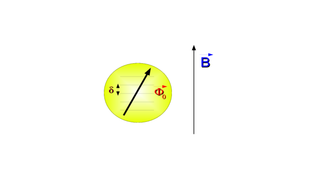
Here is a unit vector along the direction of and . The first part of the action in Eq.9 describes the coupling of non-interacting electrons to a time varying magnetic field (exchange field) of magnitude and direction . The resulting bosonic action in Eq.9 is non-abelian due to the non commutativity of the Pauli matrices. Note that the problem is ’isotropic’ in the sense that the outcome should not depend on the initial and final direction of .
We are guided by the idea that close to Stoner instability the amplitude of the exchange field is large, i.e., a large total spin develops on the dot (). In that situation one can distinguish between the adiabatic and the non-adiabatic paths of . The former involve Matsubara frequencies such that . We argue that the non-adiabatic paths do not contribute considerably to the partition function (except for providing for proper normalization), since the electrons do not manage to react to the fast changes of . Hence, we concentrate on the adiabatic paths and perform an expansion in the time variation of . We transform to a coordinate system in which coincides with the -axis
| (10) |
where is a unitary rotation matrix. Eq. (10) identifies as an element of . Indeed, if we employ the Euler angle representation
| (11) |
then the angles and determine the direction of , while is arbitrary, i.e., the condition (10) is achieved with any value of . Thus, represents the gauge freedom of the problem. We obtain
| (12) |
In the transformation (12) one can, in the spirit of Ref. [11], think of as being applied to the fermionic field. That is, one first introduces via and, then, integrates over . In this case it is convenient to choose the gauge so that remains periodic in Matsubara time upon a continuous change of to . Then is anti-periodic as it should be. This can be achieved, e.g., by fixing the gauge as . In what follows we work in this gauge.
Next, we represent the amplitude of the exchange field as a sum of its zero frequency component and of the rest, , such that . It is clear and can be easily checked that adiabatic longitudinal fluctuations do not contribute substantially to the effective action (see A for a more formal treatment). Thus, we disregard that part of and obtain
| (13) |
where
is the Berry’s connection operator in the gauge .
3 Expansion in powers of the Berry connection
In this section we perform a perturbation expansion in powers of the operator ,
and obtain an effective action which encompasses both the longitudinal
fluctuations and the Berry phase term.
We aim at the expansion of the action (9) in powers of the Berry connection operator (see LABEL:Inv7). It is expected that this expansion quickly converges for the adiabatic paths of . We write . The zeroth order term can be obtained by calculating the grand canonical potential of the noninteracting electrons subject to a constant Zeeman field . We obtain
| (15) |
where
| (16) |
Here is the partition function of noninteracting electrons subject to a magnetic field of amplitude . To determine the -dependent part of we calculate
| (17) |
where and is the Fermi distribution function. At zero temperature is the number of orbital levels between and . Assuming a constant density of states (equidistant spectrum) we obtain
| (18) |
Strictly speaking (18) is valid at temperatures higher than the level spacing , i.e., for . At lower temperatures step-like dependencies are expected. Yet, in a ”coarse-grained” sense (18) holds at lower temperatures as well. Finally,
| (19) |
where . As we consider the regime close to Stoner instability, we have . Realistically, the quantum dots are disordered and the assumption of an equidistant spectrum is too naive [17]. Due to disorder we should have
| (20) |
where is the average density of states. This question was originally addressed by Kurland et al. [1] and was recently analyzed by Burmistrov et al. [17]. Roughly, is of order . In the present paper we disregard disorder.
3.1 The first order contribution
In the first order in (Eq. LABEL:Inv7) we obtain
| (21) |
where and are the fermionic Matsubara frequencies. Calculating the sum over we obtain
| (22) |
From we conclude that
| (23) |
where was defined in Eq. (17). The contribution to the effective action, given by Eq.23, is proportional to the Berry phase. The coefficient in front of the Berry phase is roughly equal to the the number of single occupied levels, i.e., the number of uncompensated spins which acquire the Berry phase.
3.2 The second order contribution
To calculate the second order contribution we introduce the notations and and we obtain
| (24) |
Here and are bosonic Matsubara frequencies. For the transverse, i.e., the spin flipping part of , we obtain
| (25) |
In the adiabatic limit this gives
| (26) |
Hence, substitution of Eq.LABEL:Inv7 leads to the result
| (27) |
where is the angular velocity describing the motion of the magnetization vector on the sphere.
For the longitudinal part of we obtain
| (28) |
Finally . Both this terms are . In comparison of (23) is . Thus for all adiabatic frequencies the Berry’s phase action dominates. In what follows we restrict ourselves to the first order, Berry phase, contribution .
4 Partition function and magnetic susceptibility
In this section, after performing the path integration over the adiabatic paths of ,
we obtain the partition function of the problem as a function of only. This allows
us to calculate the magnetic susceptibility consisting of the Pauli and Curie terms.
Above we have obtained the following effective action for the adiabatic paths
| (29) |
This action governs fluctuations at low frequencies . Thus, at these frequencies the system reduces to a large spin of amplitude . Indeed the last term of the action (29) is just the well known Wess-Zumino action of a free spin. While a partition function of a true free spin is trivial to calculate, our spin ”lives” only at the adiabatic frequencies. We, thus, define our functional integral for the partition function as an integral over all paths whose frequency scale is cut off by . We have
| (30) |
In Eq.30 the index defines a lattice partition of the interval defined so as to limit frequencies to values . The measure is an ordinary Cartesian measure. The Hubbard-Stratonovich transformation and integrating out the fermions produce the following normalization factor
| (31) |
Here and is the number of positive Matsubara frequencies taken into account (those that are below the cut off ).
4.1 Calculating the path integral
We are guided by the idea that the most important paths are those of almost constant radius . Indeed, as can be seen from (29) the longitudinal fluctuations are suppressed by a factor containing the bare . By contrast, close to the Stoner instability, the zero frequency amplitude is only weakly suppressed (). The larger is , the bigger is the phase volume of possible transverse fluctuations. The latter are only “penalized” by the Berry phase term. An entropic “phase space” argument, outlined above, reveals that should assume a large value. Below we find out that the typical value of is of the order of , whereas we have and . To derive all these, we begin by converting the measure to a polar one, which is then adjusted to an integration over paths of almost constant radius :
| (32) |
where in the last identity we have dropped the term in the exponent
| (33) |
Here is the ultra-violet cutoff. Taking consistently the adiabatic cutoff we observe that this term is negligible in comparison with the term in the action (29).
We now perform the Gaussian integration over the longitudinal fluctuations , the net effect of which is the partial cancellation of the normalization factor (31) by . We are left with
| (34) |
We next proceed to the integral over the transverse fluctuations, i.e., the fluctuations of . These fluctuations are “penalized” by the Berry phase term in the action. The Berry phase term is given by the solid angle swept by the path. Since (this has to be checked for self consistently), these solid angles must remain small, and we can restrict ourself to a Gaussian expansion around a static value of , namely , the relevant paths will be given by the small variations around this static . At the end we should average over all possible directions of .
The Gaussian integration is easily performed if we note that the integration measure is given by . Thus, introducing we obtain
| (35) |
In evaluation of the integral we extended the integration limits of both and to even though, e.g., . This is justified for . Thus we obtain
| (36) |
The product appearing in Eq. 36 is cutoff at , i.e., at . This hard cutoff is an artifact of our rather hand-waving approach. Within this method we have no way to determine what kind of cut off should be employed. One possibility, which is supported by the calculation in Cartesian coordinates provided in B, is to use a soft cut off. This gives
| (37) |
Evidently, employing a different cut off, one would obtain a result which is different in the exponential. For example, the hard cut off gives in the exponent. This would slightly modify the numerical coefficients in the final result for the susceptibility. We keep here the soft cut off result, as it is supported by the calculation in B, and provides an excellent approximation to the exact solution [10].
We approximate the factor in (36) by 1, which is legitimate near the Stoner transition. Finally, integrating over we obtain
| (38) |
4.2 Magnetic susceptibility
We obtain the magnetic susceptibility using Eq.38 as follows
| (39) |
We observe that it consists of a Pauli and a Curie contribution. In comparison the exact solution of Ref. [10] reads
| (40) |
and the magnetic susceptibility
| (41) |
In close vicinity to the Stoner instability, i.e., the extra factor in is immaterial and we obtain an extremely good approximation to the exact result.
The Pauli-like (with an upward renormalized g-factor) susceptibility (first term in Eq. (39)) dominates when . In the low temperature regime, , the Curie-like part (second term) dominates. In this regime the average spins scales as . This Curie like contribution in the magnetic response can be tested in materials close to the Stoner instability such as Pd () or () [8]. It is important to understand that the Curie part of the susceptibility represents a mesoscopic effect. The density of states of a QD scales linearly with the volume of the dot, . On the other hand . Hence the Pauli like part of the magnetic susceptibility is proportional to the volume and is an extensive quantity. On the other hand, the Curie susceptibility is intensive as is scale invariant. Therefore for a fixed temperature , if one gradually increases the size of the system, the Pauli part grows and, eventually, the Curie susceptibility becomes negligible compared to the Pauli one.
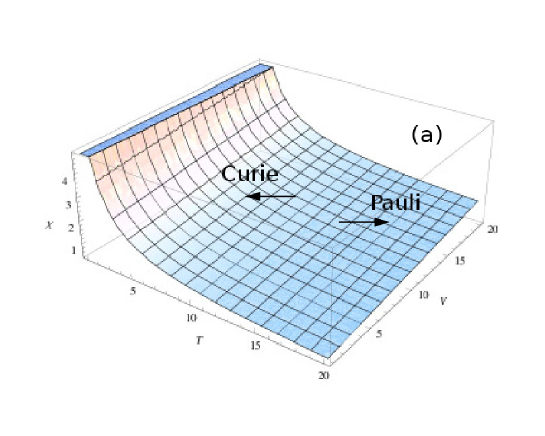
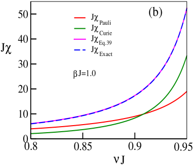
This behavior is shown in Fig.2(a) where is chosen to be in close vicinity of the Stoner instability regime. To illustrate the nature of Pauli and Curie like suceptibility more, we show their behavior as a function of the Stoner parameter in Fig. 2(b). It is clear that for a fixed dimensionless parameter , the Curie susceptibility (green curve) becomes more dominant over the Pauli one (red curve) as we approach towards the Stoner instability point. On the other hand, the blue curve shows the behavior of which in close vicinity to the Stoner instability point matches quite well to our approximate answear (Eq. (39)), shown by the magenta curve in Fig. 2(b).
5 Summary and Discussion
In this paper we have considered an isolated QD with an isotropic exchange interaction. In the path integral HS formulation this problem leads to an effective non-abelian action. Here we have presented an approximative geometric approach in which the Berry phase controls the dynamics of the direction of the HS magnetization vector . Close to the Stoner limit, i.e., for , our approach reproduces well the exact solution of Ref. [10] which comes at the expense of a hard calculation based on the generalized Wei-Norman-Kolokolov method [16]. Note that even zero frequency observables (for e.g. susceptibility), involve summation over finite frequency fluctuations (Eq. (57)), including both low and high frequency contributions. Although the exact result describes both the low and high energy contents of susceptibility, we here show that if one is interested in the low energy regime of long range fluctuations, the information of the exact result can be obtained from our physically motivated and user friendly approach of the invariant action. However if one insists on knowing ultraviolett behavior, then one may resort to an equally simple gaussian expansion around stationary points. Hence, our approximative geometric approach covers much of the contents of the observable, in a manner suitable for further generalization. Therefore, we believe that this approach could be very useful in situations in which the exact method is inapplicable. These may be, e.g., the problems of charge and spin transport via quantum dots coupled to normal or ferromagnetic leads.
Strictly speaking our results are valid for . Yet, for the equidistant spectrum assumed in this paper we do not expect major changes at lower temperatures. In the presence of disorder the low temperature regime is itself more subtle [17].
Finally, it is important to mention that, as discussed around Eq. (20), disorder can influence the grand canonical potential of non-interacting electrons quite essentially. Yet, it is easy to show that the Berry phase part of the action is quite insensitive to disorder.
6 Acknowledgments
This work was supported by GIF, Einstein Minerva Center, Sonderforschungsbereich TR 12 of the Deutsche Forschungsgemeinschaft, EU FP7 grant GEOMDISS, the Russian-Israel scientific research cooperation (RFBR Grant No. 11-02-92470 and IMOST 3-8364), the Council for Grant of the President of Russian Federation (Grant No. MK-296.2011.2), RAS Programs “Quantum Physics of Condensed Matter” and “Fundamentals of nanotechnology and nanomaterials”, the Russian Ministry of Education and Science under contract No. P926.
We acknowledge useful discussions with Gabriele Campagnano, Igor Lerner, Mikhail Kiselev, Jürgen König and Alexander Mirlin. We are grateful to Ganpathy Murthy for providing us with notes of his calculations on ”Universal interacting crossover regime in two-dimensional quantum dots“ (Ref.[21]) and a detailed explanation.
Appendix A Unimportance of longitudinal fluctuations
Here we show why the longitudinal fluctuations of can be disregarded.
Following the spirit of Ref. [11] we gauge out in Eq. (12) the fluctuations by using a (non-unitary) transformation , where . We obtain
| (42) |
where
This means that, in fact, appearing in (LABEL:Inv7) is the expression (LABEL:Inv7aa). We observe that the longitudinal part of of (LABEL:Inv7aa), which is responsible for the Berry phase term in the action, does not contain the operators and, thus, is not influenced by the longitudinal fluctuations which appear only in the factor . Moreover, substituting of (LABEL:Inv7aa) into Eq. (26) we observe that in the adiabatic limit the longitudinal fluctuations drop out also in the second order terms. Thus, disregarding the longitudinal fluctuations in (13), and the factor altogether, was justified.
Appendix B Expansion in small transverse fluctuations
Here we present an alternative method of calculating the path integral in Cartesian coordinates. The advantage is the higher level of accuracy in handling the integration measure. An adiabatic cut off need not be postulated here. Rather, a soft adiabatic cut off appears naturally.
B.1 Effective action
We start from the Hamiltonian (6) and rewrite the action (7) in the Matsubara representation as
| (44) |
We apply the HS transformation on Eq.44 to obtain an effective action quadratic in the fermionic fields, with an auxiliary vector bosonic field () for the spin degrees of freedom. Hence, the effective action reads
| (45) |
where the Matsubara expansion for the bosonic HS real vector field reads
| (46) |
Here is the zero component of the bosonic HS real vector field and are the non-zero ones.
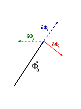
Our strategy is to, first, integrate over the non-zero Matsubara components while keeping fixed and, then, integrate over all possible . The vectors have three components among which one is longitudinal and the other two are the transverse with respect to the current direction of , which is schematically shown in Fig.3. Moreover we choose the basis for in accordance with the direction of , i.e., the axis for is along . In other words for the time being we break the symmetry of the isotropic problem choosing a particular direction of and select the basis for in accordance with the current direction of . Note that at the end of the day one should integrate over all in order to restore the global symmetry of the problem and obtain an expression for the partition function and the susceptibility compatible with Eqs.38 and 39. In terms of and the cartesian fluctuations around it, Eq.45 can be rewritten as
| (47) |
where is the single particle Green’s function of the electrons subject to a constant magnetic field . For the partition function we obtain
| (48) |
Integrating out the fermions we obtain
| (49) |
where the effective action depends on and and can be written as
| (50) |
Here stands for combined time (Matsubara frequencies) and spin trace.
B.2 Expansion to the second order in fluctuations
We expand the effective action (Eq.50) up to the second order in the fluctuations . The zeroth order contribution has already been calculated in Sec. 3. It is easy to show that the first order contribution vanishes and we obtain
| (51) |
After a straightforward calculation this gives
where and was defined after Eq. (23). Similar expression was obtained earlier in Ref. [21] for a more involved regime of strong spin-orbit coupling. The last term of (B.2) is purely imaginary and, at low frequencies (adiabatic condition ), corresponds to the Berry phase. Substituting Eq.B.2 into Eq.51 we obtain
| (53) |
where
| (54) | |||||
At this point we can perform the Gaussian integration over . We obtain
| (55) |
where is a -independent and -independent normalization.
Thus we see that close enough to Stoner instability, i.e., for , we reproduce Eqs. (37) and (38). Indeed, this is so if we are allowed to replace
| (56) |
for all relevant . This approximation works, at least, in the regime of relatively high temperatures, i.e., when . In this case the integral (38) is dominated by and we obtain .
B.3 Restoring the Goldstone mode in Cartesian coordinates
Having already reproduced the results of the main text we would like to improve our understanding as well as the precision of the calculation by analyzing Eq. 53 and Eq. 54 a bit closer. We rewrite Eq. 54 as
| (57) | |||||
The second term of the RHS of (57) is problematic since it gives a finite ”mass” for the transverse fluctuations. Yet, from the spherical symmetry we should expect a Goldstone mode and no ”mass”. However, the origin of this term is quite clear. It can be nicely rewritten as
| (58) |
Here is the prolongation of the zero mode vector due to transverse fluctuations. This term combines with the term of (53) to give , where . Thus we ”loose” the Goldstone mode because we use Cartesian coordinates and not the spherical ones where would be kept constant. This term could be just subtracted thus recovering the Goldstone physics and reducing back to . We distinguish two regimes:
-
(A)
At high frequencies the action (57) reduces (with no subtractions) to(59) In this limit the integration over the Gaussian fluctuations produces a factor per Matsubara frequency, which compensates the factor per Matsubara frequency in Eq. (48). Thus it is not necessary to subtract anything at high frequencies.
-
(B)
In this limit, after the subtraction of the second term of the RHS of (57) and retaining only transverse fluctuations we obtain(60) In the time representation Eq.60 reads
(61) The first term in Eq.61 is equal to the Berry phase term (23). The second term is of the second order in derivatives and can be rewritten as
(62) where is the unit vector in the direction of . Thus we reproduce the second order term (27). Since the obtained action is local in time and is proportional to the time derivatives, the fact that we started from an expansion in small fluctuations around a given is no longer important. Indeed, we can always choose the direction of close to the ”current” .
B.4 Calculation with a proper counter term
As we have seen we have to subtract the ”mass” term only for the adiabatic frequencies. Here we propose a particular form of the counter term which satisfies this condition. We rewrite again Eq. 54 as , where
| (63) | |||||
and
| (64) |
The splitting is chosen so that represents the ”mass” term at adiabatic frequencies but vanishes at high frequencies. We subtract the counter term . Then we obtain
| (65) | |||||
Close to Stoner instabilty, i.e., for , we can approximate the second multiplier (in rectangular brackets) by and we reproduce the result (38) and (39) from there. In this approach no limitation on temperature from below appears.
Appendix C QD in presence of an external magnetic field B
Here we provide an alternative derivation of the susceptibility by considering the isolated QD in a weak magnetic field. Unlike in the previous calculation, here the normalization factors of the path integral are not important.
In the presence of a constant magnetic field B the Hamiltonian of the QD can be written as
| (66) |
Following the same procedure as described in B.1 we derive the effective action for this situation. The constant magnetic field adds to the zero frequency component of the exchange field and, effectively, the new field plays the role of in the calculation. We obtain
| (67) |
where in is the single particle Green’s function of the electrons in presence of B and . Here is the angle between B and .
We again expand up to the second order in fluctuations and obtain
| (68) |
Following the same steps as described in B.2 and B.3 we obtain the partition function
| (69) |
The susceptibility is now given by
| (70) |
Performing the appropriate saddle point approximation (up to the quadratic fluctuations around the saddle point) we obtain the susceptibility given in Eq. 39.
References
- [1] I. L. Kurland, I. L. Aleiner, B. L. Altshuler, Mesoscopic magnetization fluctuations for metallic grains close to the stoner instability, Phys. Rev. B 62 (22) (2000) 14886–14897.
- [2] I. L. Aleiner, P. W. Brouwer, L. I. Glazman, Quantum effects in coulomb blockade, Physics Reports 358 (2002) 309–440.
- [3] Y. Alhassid, The statistical theory of quantum dots, Rev. Mod. Phys 72 (4) (2000) 895.
- [4] A. V. Andreev, A. Kamenev, Itinerant ferromagnetism in disordered metals: A mean-field theory, Phys. Rev. Lett. 81 (15) (1998) 3199.
- [5] E. C. Stoner, Ferromagnetism, Rep. Prog. Phys. 11 (1947) 43.
- [6] P. Gambardella et al, Giant magnetic anisotropy of single cobalt atoms and nanoparticles, Science 300 (2003) 1130.
- [7] G. E. Mpourmpakis et al, Role of co in enhancing the magnetism of small fe clusters, Phys. Rev. B 72 (2005) 104417.
- [8] S. Jia, S. L. Budko, G. D. Samolyuk, P. C. Canfield, Nearly ferromagnetic fermi-liquid behaviour in and high-temperature ferromagnetism of , Nature Phys. 3 (5) (2007) 334.
- [9] M. N. Kiselev, Y. Gefen, Interplay of spin and charge channels in zero-dimensional systems, Phys. Rev. Lett. 96 (2006) 066805.
- [10] I. Burmistrov, Y. Gefen, M. Kiselev, Spin and charge correlations in quantum dots: An exact solution, Pis’ma v ZhETF 92 (3) (2010) 202.
- [11] A. Kamenev, Y. Gefen, Zero-bias anomaly in finite-size systems, Phys. Rev. B 54 (8) (1996) 5428.
- [12] K. B. Efetov, A. Tschersich, Coulomb effects in granular materials at not very low temperatures, Phys. Rev. B 67 (2003) 174205.
- [13] N. Sedlmayr, I. V. Yurkevich, I. V. F. Lerner, Tunneling density of states at coulomb-blockade peaks, Europhys. Lett. 76 (2006) 109–114.
- [14] Y. Alhassid, T. Rupp, Effects of spin and exchange interaction on the coulomb-blockade peak statistics in quantum dots, Phys. Rev. Lett. 91 (5) (2003) 056801.
- [15] G. Usaj, H. U. Baranger, Exchange and the coulomb blockade: peak height statistics in quantum dots, Phys. Rev. B 67 (2003) 121308.
- [16] I. V. Kolokolov, A functional integration method for quantum spin systems and one-dimensional localization, Int. J. Mod. Phys. B 10 (18) (1996) 2189.
- [17] I. S. Burmistrov, Y. Gefen, M. N. Kiselev, An exact solution for spin and charge correlations in quantum dots: The effect of level fluctuations and zeeman splitting, arXiv:1201.4641 [cond-mat.mes-hall].
- [18] M. Schechter, Spin magnetization of small metallic grains, Phys. Rev. B 70 (2004) 024521.
- [19] S. Schmidt, Y. Alhassid, K. van Houcke, Effect of a Zeeman field on the transition from superconductivity to ferromagnetism in metallic grains, Europhys. Lett. 80 (2007) 47004.
- [20] S. Schmidt, Y. Alhassid, Mesoscopic competition of superconductivity and ferromagnetism: Conductance peak statistics for metallic grains, Phys. Rev. Lett. 101 (2008) 207003.
- [21] G. Murthy, Universal interacting crossover regime in two-dimensional quantum dots, Phys. Rev. B 77 (2008) 073309.