Phantom Inflation in Little Rip

Abstract

We study the phantom inflation in little rip cosmology, in which the current acceleration is driven by the field with the parameter of state $w<-1$, but since $w$ tends to -1 asymptotically, the rip singularity occurs only at infinite time. In this scenario, before the rip singularity is arrived, the universe is in an inflationary regime. We numerically calculate the spectrum of primordial perturbation generated during this period and find that the results may be consistent with observations. This implies that if the reheating happens again, the current acceleration might be just a start of phantom inflation responsible for the upcoming observational universe.

I Introduction

The phantom field, in which the parameter of the equation of state $w<-1$, has still acquired increasingly attention [1], inspired by the study of dark energy, e.g. [2],[3],[4],[5],[6],[7],[8],[9],[10]. The actions with phantomlike behavior may be arise in supergravity [11], scalar tensor gravity [12], higher derivative gravity [13], braneworld [14], string theory [15], and other scenarios [16, 17], and also from quantum effects [18]. The universe driven by the phantom field will evolve to a singularity, in which the energy density become infinite at finite time, which is called the big rip, see Refs.[19],[20],[21],[22],[23],[24] for other future singularities .

Recently, the little rip scenario has been proposed [25], in which the current acceleration of universe is driven by the phantom field, the energy density increases without bound, but $w$ tends to -1 asymptotically and rapidly, and thus the rip singularity dose not occur within finite time. This scenario still leads to a dissolution of bound structures at some epochs [25, 26], which is similar to the big rip, however, in little rip scenario, the universe arrives at the singularity only at infinite time. This has motivated some interesting studies [27], and also asymptotically phantom dS universes or pseudo-rip [28],[29].

The simplest realization of phantom field is the scalar field with reverse sign in its dynamical term. In little rip scenario, initially $w<-1$, the energy density of the phantom field will increase with time, and arrive at a high energy scale at finite time, and at this epoch the phantom field has $w\simeq-1$. Thus after some times or before the rip singularity of universe is arrived, if the exit from the little rip phase and the reheating happen, the inflation, which is driven by the phantom field, in little rip phase might be responsible for the upcoming observational universe.

The phantom inflation has been proposed in [30], and also in [31],[32],[33],[34],[35],[36],[37],[38],[39]. Recently, there has been a relevant study in modified gravity [40]. In phantom inflation scenario, the power spectrum of curvature perturbation can be nearly scale invariant. The duality of primordial spectrum to that of normal field inflation has been studied in [31, 41]. The exit from the phantom inflation has been studied [30],[32],[36],[37],[38]. The spectrum of tensor perturbation in phantom inflation is slightly blue tilt [30],[42], which is distinguished from that of normal inflationary models.

Here, we will argue that after a finite period of the little rip phase the universe might recur the evolution of observational universe. We will calculate the spectrum of primordial perturbation during the phantom inflation in various little rip phases, and find that the spectrum may be consistent with observations. We discussed the implication of this result in the final.

II The phantom inflation in little rip

In little rip phase, initially $w<-1$, the energy density of the phantom field will increase with time, and arrive at a high energy scale at finite time, and at this epoch the phantom field has $w\simeq-1$. Here, we actually required that before $w\simeq-1$, the phantom field must have arrived at a high energy regime, which assures the occurrence of inflation. In general, this can be implemented by introducing a monotonically increasing potential of the phantom field.

The phantom field satisfies the equations

$$3H^{2} = -\frac{1}{2}\dot{\phi}^{2}+V(\phi),$$ (1)

$$\ddot{\phi} + 3H\dot{\phi}-V_{\phi}(\phi)=0,$$ (2)

where $M_{P}^{2}/8\pi=1$, and the dot is the derivative with respect to the physical time $t$. $H^{2}>0$ requires that in all case for the phantom evolution $\dot{\phi}^{2}$ must be smaller than its potential energy. The phantom field will be driven to climb up along its potential, which is reflected in the minus before $V_{\phi}$ term. We define the slow climbing parameters [30], as for normal inflation.

$$\epsilon_{Pha}\equiv-\frac{\dot{H}}{H^{2}}<0~{}~{}~{},~{}~{}~{}\delta_{Pha}\equiv-\frac{\ddot{\phi}}{H\dot{\phi}}.$$ (3)

Thus the equation of state is

$$w_{Pha}={2\over 3}\epsilon_{Pha}-1.$$ (4)

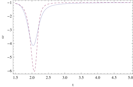
Figure 1: The evolutions of $w$ with the time for $V(\phi)\sim\phi^{2}$ (solid line) and $\phi^{3}$ (dashed line), respectively, where $\phi$ is the phantom field, which is initially around the bottom of its potential.

We consider the monotonically increasing potential of the phantom field as $V(\phi)\sim\phi^{N}$. The phantom field initially drives the current acceleration, and is in low energy regime with $w\simeq-1$. Then the field will climb up along its potential, $w$ will rapidly deviate from $-1$ during this period. However, when the phantom field climbs to $\phi\simeq 1$, $|\epsilon_{Pha}|\sim 1$. Hereafter, the conditions $|\epsilon_{Pha}|<1$ and $|\delta_{Pha}|<1$ are satisfied, since

$$\left|\epsilon_{Pha}\right|=\frac{\dot{H}}{H^{2}}\sim{N^{2}\over\phi^{2}},$$ (5)

which is smaller for larger $\phi$. Thus $w\simeq-1$ is obtained again, which is the phantom inflationary phase, since the phantom field is in high energy regime. Thus in the little rip cosmology, it is generally that before the the universe arrives at the singularity, it will enter into a period of the phantom inflation, up to the singularity at infinite time.

Figure 2: The sketch of the exit from little rip phase. $\phi$ is the phantom field, while $\psi$ is the normal waterfall field, as that in hybrid inflation [43],[44]. Initially $\phi$ is at the bottom of its potential, which then climbs up along its potential. The effective $M^{2}_{\psi}$ of $\psi$ is initially positive, which will gradually decrease with the increasing of $\phi$. When $\psi$ becomes tachyonical, and $\psi$ will rapidly roll down along its potential. Thus at this time almost all energy of $\phi$ will be released.

The evolutions of $w$ are plotted in Fig.1 for the potential $\phi^{N}$. The result is consistent with above discussions.

However, it is possible that some times after the energy density of the phantom field arrives at a high energy scale, or before the rip singularity of universe is arrived, the energy of field will be released, and the universe reheats, after which the evolution of hot “big bang” recurs. The exit mechanism in Ref.[30] is depicted in Fig.2.

However, before the phantom field arrives at the high energy regime responsible for inflation, if the exit from the little rip phase or the reheating happens, the phantom inflation will not exist. Thus whether the phantom inflation occur will depend on the exiting scale from little rip phase. Here, we require this exiting scale is at least about $M\sim\rho_{inf}^{1/4}\sim 10^{-3}$, $\rho_{inf}\sim 10^{-12}$ is the inflationary energy density. Before this, the current bound structures have disintegrated, see Appendix A.

III The spectrum of primordial perturbation

III.1 Basic results

We will calculate the spectrum of curvature perturbation during the phantom inflation. We define [45],[46]

$$u=-z\mathcal{R}$$ (6)

where $\cal R$ is the curvature perturbation, and $z\equiv a\sqrt{2|\epsilon_{Pha}|}$.

The motive equation of $u_{\rm k}$ in the $k$ space is

$$u_{\rm k}^{\prime\prime}+\left(k^{2}-\frac{z^{\prime\prime}}{z}\right)u_{\rm k}=0,$$ (7)

where the prime is the derivative with respect to conformal time. In general, when $k^{2}\gg z^{\prime\prime}/z$, the solution of perturbation is

$$u_{{\rm k}}\sim\frac{1}{\sqrt{2k}}\,e^{-ik\eta}\,.$$ (8)

The $\frac{1}{\sqrt{2k}}$ is obtained by the normal quantization of mode function $u_{k}$, which seems illogical for phantom field, since there is a ghost instability induced by $\epsilon<0$. However, it might be thought that the evolution with $w<-1$ emerges only for a period, which may be simulated phenomenologically by the phantom field, while the full theory should be well behaved. It has been showed in Ref.[47] that $\epsilon$ can be replaced with $|\epsilon|$, due to the introduction of generalized Galileon field [48],[49], there is not the ghost instability, the perturbation theory is healthy.

While $k^{2}\ll z^{\prime\prime}/z$, the dominated mode is

$$u_{{\rm k}}\sim z\$$ (9)

which means that the curvature perturbation $|{\mathcal{R}}_{{\rm k}}|=|u_{{\rm k}}/z|$ is constant in this regime.

The power spectrum ${\cal P}_{{\cal R}}(k)$ is defined as

$$\langle{\cal R}_{{\rm k}_{1}}{\cal R}^{*}_{{\rm k}_{2}}\rangle=\frac{2\pi^{2}}{k^{3}}{\cal P}_{{\cal R}}\delta^{3}\,(k_{1}-k_{2})\,,$$ (10)

and is given by

$${\cal P}_{{\cal R}}^{1/2}(k)=\sqrt{\frac{k^{3}}{2\pi^{2}}}\,\left|\frac{u_{{\rm k}}}{z}\right|\,.$$ (11)

In slow climbing approximations $|\epsilon_{Pha}|\ll 1$ and $|\delta_{Pha}|\ll 1$,

$$\mathcal{P}_{\mathcal{R}}^{1/2}=\frac{1}{\sqrt{2|\epsilon_{Pha}|}}\frac{H}{2\pi},$$ (12)

where the spectral index is

$$n_{\mathcal{R}}-1\simeq-4\epsilon_{Pha}+2\delta_{Pha}.$$ (13)

Noting the spectral index is only determined by $\epsilon_{Pha}$ but not its absolute value, since we have $|\epsilon_{Pha}|^{\prime}/|\epsilon_{Pha}|=\epsilon_{Pha}^{\prime}/\epsilon_{Pha}$ and $|\epsilon_{Pha}|^{\prime\prime}/|\epsilon_{Pha}|=\epsilon_{Pha}^{\prime\prime}/\epsilon_{Pha}$ in the calculation of $\frac{z^{\prime\prime}}{z}$.

This spectrum may be either blue or red. The results are dependent on the relative magnitude of $\epsilon_{Pha}$ and $\delta_{Pha}$, see Ref.[30] for the details.

In big rip scenario, the big rip singularity requires $w_{Pha}<-1$, the primordial spectrum obtained is not scale invariant, unless $w_{Pha}$ is not far from $-1$. While in little rip cosmology, $w_{Pha}$ tends to -1, thus with the increasing of time we certainly have $|\epsilon_{Pha}|\ll 1$, which naturally insure the scale invariance of spectrum.

III.2 Numerical results

Here, we will calculate ${\cal P}_{{\cal R}}$ by evolving the full mode equation (7) numerically without any approximations.

We define $\alpha=\ln{a}$, and with this replacement, we have

$$H_{\alpha}=\frac{1}{2}H\phi_{\alpha}^{2},$$ (14)

$$\phi_{\alpha\alpha}+(\frac{H_{\alpha}}{H}+3)\phi_{\alpha}-\frac{1}{H^{2}}V_{\phi}=0.$$ (15)

where the subscript $\alpha$ is the derivative for $\alpha$, which will facilitate the numerical integration. The perturbation equation (7) can be written as

$$u_{\alpha\alpha}+(1+\frac{H_{\alpha}}{H})u_{\alpha}+\left(\frac{k^{2}}{e^{2\alpha}H^{2}}-\frac{z^{\prime\prime}/z}{e^{2\alpha}H^{2}}\right)u=0,$$ (16)

where $\frac{z^{\prime\prime}}{z}$ is only the function of $H$ and its higher order derivative with respect to $\alpha$, which here will be determined by the numerical calculation.

It has been clearly explained in Refs.[25],[26] that before the rip singularity is arrived, the little rip universe experiences the disintegration of bound structures. Hence, actually in finite time, the universe becomes totally empty. However, the asymptotical behavior of the evolution of $a$ is significant to determine the character of perturbation spectrum generated during this period.

The solution of Eq.(16) is only determined by the behavior of $a$. Thus in principle, for any parametrization of $a$ depicting the little rip phase, the corresponding power spectrum can be calculated. The details of the implement of field theory dose not significantly alter the result of Eq.(16), unless its speed of sound is rapidly changed. Below, we will focus on some interesting parametrizations of $a$. We will study some cases with the phantom potential in Appendix B.

We firstly consider the parametrization of little rip in Refs.[25],[26]

$$H=\,H_{0}e^{\lambda t},$$ (17)

where $H_{0}$ and $\lambda$ are constant, which implies

$$a \sim e^{{H_{0}\over\lambda}e^{\lambda t}},$$ (18)

$$w = -1-{2\lambda\over 3H_{0}}e^{-\lambda t}.$$ (19)

Thus $w\simeq-1$ for $\lambda t\gg 1$, and there is not curvature singularity at finite time. In Ref.[25], in low energy regime the parameters chosen can make a best fit to the latest supernova data. However, we are interested in the evolution in a high energy regime with $w\simeq-1$, in which $\lambda t\gg 1$.

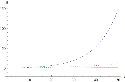
Figure 3: The evolutions of $H$ in Eq.(17) for $\lambda=0.1$ (the dashed line), 0.05 (the dotted line), 0.02 (the solid line), respectively.

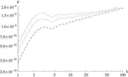
Figure 4: The power spectrum of curvature perturbation corresponding to the evolutions of $H$ in Fig.(3), respectively.

The evolution of $H$ with this parametrization is plotted in Fig.3. The power spectrum is plotted in Fig.4. It seems that the spectrum is nearly scale invariant only for small $\lambda$. However, this result is dependent on the time interval selected. In principle, as long as $\lambda t$ is enough large, the spectrum can be scale invariant for any $\lambda$. It seems there is a cutoff $k_{cutoff}$ in Fig.4, however, which appears is because initially there are some perturbation modes outside of the horizon. This cutoff can be changed with the difference of the initial parameters in the numerical calculation.

Then we consider the parametrizations of $a$ in e.g.Ref.[29] for asymptotically phantom dS universes. The first is

$$a(t)\sim e^{\frac{x_{f}t}{\sqrt{3}}}e^{g(t)},$$ (20)

$$g(t)=\frac{2x^{2}_{f}}{3b}(1-\frac{x_{0}}{x_{f}})(e^{-\frac{\sqrt{3}bt}{2x_{f}}}-1),$$ (21)

where $x_{0},x_{f},b$ are constant and $x_{f}>x_{0}$. The second is

$$a(v)\sim\frac{1}{(1-v^{\frac{3}{2}})^{2/3\gamma}},$$ (22)

$$t(v)=t_{0}-\frac{2}{\sqrt{3}\gamma x_{f}}ln(1-v),$$ (23)

where $x_{f},\gamma$ are constant, and the parameter $v$ varies from $0(t=t_{0})$ to $1(t\rightarrow\infty)$. In Ref.[29], the realizations of field theory have been given. Here, what we require is only the evolutions of $a$. In fact, both cases have similar behavior. The parameter $H$ grows at the beginning and asymptotically tends to constant at late time, see Fig.5. The power spectrum is plotted in Fig.6. The spectrums are nearly scale invariant and are slightly blue tilt. We see that the smaller $x_{f}$ is for the parametrization (20), the flatter the spectrum is, and the smaller $\gamma$ is for the parametrization (22), the flatter the spectrum is.

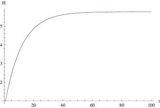
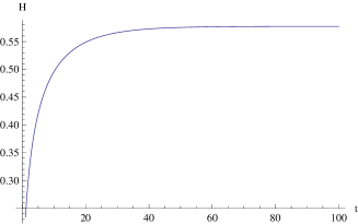
Figure 5: The evolution of $H$. The upper panel corresponds to the parametrization (20) for $x_{0}=1,b=1,x_{f}=10,$ and the lower panel corresponds to the parametrization (22) for $x_{f}=0.001,\gamma=10$

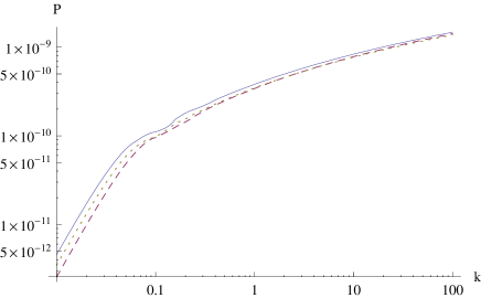
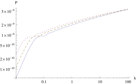
Figure 6: The power spectrum of the curvature perturbation. The upper panel correspond to the parametrization (20) for $b=1,x_{f}=5$ (solid line), $b=1,x_{f}=10$(dotted line),$b=1.5,x_{f}=4$(dashed line) and the lower panel correspond to the parametrization (22) for $x_{f}=0.001$ and $\gamma=10$(solid line), $\gamma=15$(dashed line),$\gamma=20$ (dotted line) , respectively.

We see that for all considered parametrizations, the power spectra of perturbations are nearly scale invariant, but slightly blue tilt. The results are determined by the asymptotical behavior of the evolution of $a$, which reflects how the state parameter $w$ the phantom field approaches $-1$. In principle, there might be a classification of the parametrization of $a$ in term of its giving the spectral tilts, which might be interesting for further studies.

IV Conclusion and Discussion

In effective actions of some theories, the phantom field naturally appear, which might be a suitable simulation of a fundamental theory below certain physical cutoff. The cosmology with the phantom field has been widely studied.

In little rip scenario, the current acceleration of universe is driven by the phantom field with $w<-1$, the energy density of the phantom field will increase without bound, but since $w$ tends to -1 asymptotically, there is not the rip singularity at finite time. This indicates that in little rip phase, the phantom field will inevitably arrive at a high energy scale at late time, and at this time it can have $w\simeq-1$, which corresponds to a period of phantom inflation. Thus if the exit and the reheating happens before the rip singularity of the universe is arrived, the phantom inflation in little rip phase might be responsible for the coming observational universe. Here, we have showed this possibility.

We have calculated the spectrum of primordial perturbation during phantom inflation in different little rip scenario and asymptotically phantom dS universes, and found that the results may be consistent with observations. In normal inflationary models, the spectrum of tensor perturbation is slightly red. While the phantom inflation predicts a slightly blue spectrum of tensor perturbation, which is distinguished from that of normal inflationary models, but may be consistent with observations [50, 51].

Here, the calculating method for the primordial perturbation is applicable for any parametrization of $a$. As long as $w\lesssim-1$ is satisfied in high energy regime, the spectrum will be scale invariant. However, in big rip scenario, the big rip singularity requires $w_{Pha}<-1$, the primordial spectrum is scale invariant only if $w_{Pha}$ is nearly around $-1$.

We can imagine that after the available energy of the phantom field is released, it might be placed again in initial position of its effective potential, and after the hot “big bang” universe evolves into the low energy regime, this field might dominate again and roll up again along its potential, the universe comes again to the little rip phase and the phantom inflation recurs. This brings a scenario[52],[53],[54], in which the universe expands all along but the Hubble parameter oscillates periodically. In this scenario, we live only in one cycle, the current acceleration with $w<-1$ might be just a start of phantom inflation responsible for the observational universe in upcoming cycle, and the universe recurs itself. It might be interesting to see whether this scenario is altered by the evolution of perturbation on large scale, e.g.[55],[56].

It is generally difficult to foresee the future of our universe, since there are lots of the evolutions or the parametrizations of $w$, which may be consistent with the current observations but have different aftertime, e.g.[57]. However, if the universe is recurring, the observations for the primordial perturbation might help us to see the ‘tomorrow’ of our universe.

Here, the recurring time is determined by the potential of the phantom field. However, if there is a large step in its potential, which straightly joint the current low energy regime to the regime of phantom inflation, this time will be abridged. This might leave an observational effect in upcoming universe, e.g. a lower CMB quadrupole, which will be showed in later work.

Acknowledgments

We thank Sergei D. Odintsov, Taotao Qiu for helpful discussions. This work is supported in part by NSFC under Grant No:10775180, 11075205, in part by the Scientific Research Fund of GUCAS(NO:055101BM03), in part by National Basic Research Program of China, No:2010CB832804

Appendix:A

The little rip phase will result in the disintegration of bound structures, e.g.[29]. The acceleration of the universe brings an inertial force on a mass $m$ as felt by a gravitational source separated by a comoving distance $l$,

$$F_{in}=ml\frac{\ddot{a}}{a}={ml\over 6}(2\rho(a)+\rho^{\prime}(a)a),$$ (24)

where $M_{P}^{2}/8\pi=1$ and the energy density $\rho(a)$ is the function of the scale factor. It is convenient to introduce dimensionless parameter

$${\bar{F}}_{in}={2\rho(a)+\rho^{\prime}(a)a\over\rho_{0}},$$ (25)

where $\rho_{0}$ is the dark energy density at the present time. The disintegration time of bound structures can be calculated by applying Eq.(25). In Ref.[29], it is found that the system of Sun and Earth disintegrates when ${\bar{F}}_{in}$ reaches $\sim 10^{23}$. Thus at this time

$$\rho(a)\sim 10^{23}\rho_{0}\sim 10^{-100}\ll\rho_{inf},$$ (26)

where $\rho_{inf}\sim 10^{-12}$ is the inflationary energy density. Thus the time before the phantom inflation is far larger than the remaining time for the dissolution of bound structure.

Appendix:B

We consider the potential as

$$V_{M}(\phi)=\frac{1}{2}M^{2}\phi^{2}\left(1+\beta\tanh(\frac{\phi-\phi_{Step}}{\Delta})\right).$$ (27)

This potential has a step at $\phi_{Step}$. The parameters $\beta$ and $\Delta$ determine the height and width of this step. Though there is an abrupt change of the evolution of the phantom field due to the exist of step, the phantom field will climb up continuously through the step while the phantom inflation will not be ceased.

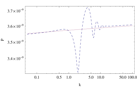
Figure 7: The power spectrum of curvature perturbation for the phantom inflation with the potential (27). The solid and dashed lines are those without and with the step, respectively.

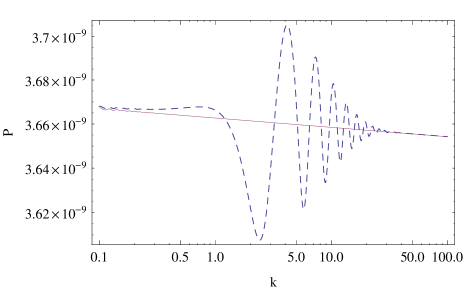
Figure 8: The power spectrum of curvature perturbation for the phantom inflation with the potential $V_{0}+V_{M}$. The solid and dashed lines are those without and with the step, respectively.

The power spectrum for the phantom inflation with this potential is plotted in Fig.7. The spectrum is scale invariant. The step in the potential will result in a burst of oscillations, and the magnitude and extent of oscillation are dependent on the height and width of the step. These oscillations might provide a better fit e.g.[58],[59].

The normal inflation model with the same potential has a red spectrum $n_{\mathcal{R}}<1$, while the phantom inflation has a blue spectrum $n_{\mathcal{R}}>1$, since

$$\epsilon_{Pha}\simeq\delta_{Pha}<0.$$ (28)

However, we can have the models of the phantom inflation with $n_{\mathcal{R}}<1$. We consider an alternative potential as $V_{0}+V_{M}$, in which $V_{M}$ is Eq.(27) and $V_{0}$ is constant dominating the potential. Here,

$$|\epsilon_{Pha}|\ll|\delta_{Pha}|,$$ (29)

and both are negative. Fig 8 shows that the spectrum is scale invariant, but has a slightly red tilt.

References

- [1] R.R. Caldwell, Phys. Lett. B545, 23 (2002).
- [2] R.R. Caldwell, M. Kamionkowski and N.N. Weinberg, Phys. Rev. Lett. 91, 071301 (2003).
- [3] P. Singh, M. Sami and N. Dadhich, Phys. Rev. D 68, 023522 (2003); M. Sami and A. Toporensky, Mod. Phys. Lett. A19, 1509 (2004).
- [4] J.G. Hao, X.Z. Li, Phys. Rev. D67, 107303 (2003).
- [5] S. Nojiri, S.D. Odintsov, Phys. Lett. B562, 147 (2003); E. Elizalde, S. Nojiri, S.D. Odintsov, Phys. Rev. D70, 043539 (2004).
- [6] Z.K. Guo, Y.S. Piao, and Y.Z. Zhang, Phys. Lett. B594, 247 (2004).
- [7] J.M. Aguirregabiria, L.P. Chimento, R. Lazkoz, Phys. Rev. D70, 023509 (2004); L.P. Chimento, D. Pavon, Phys. Rev. D73, 063511 (2006).
- [8] Kujat, R.J. Scherrer, A.A. Sen, Phys.Rev. D74 (2006) 083501.
- [9] V. Faraoni, Class. Quant. Grav. 22, 3235 (2005); J.V. Faraoni, A. Jacques, Phys. Rev. D76, 063510 (2007).
- [10] K. Bamba, C.Q. Geng, Prog. Theor. Phys. 122, 1267 (2009); K. Bamba, M. Jamil, D. Momeni, R. Myrzakulov, arXiv:1203.2103; K. Bamba, K. Yesmakhanova, K. Yerzhanov, R. Myrzakulov, arXiv:1203.3401.
- [11] H.P. Nilles, Phys. Rept. 110 1 (1984).
- [12] B. Boisscau, G. Esposito-Farese, D. Polarski and A.A. Starobinsky, Phys. Rev. lett. 85 2236(2000).
- [13] M.D. Pollock, Phys. Lett. B215, 635 (1988).
- [14] V. Sahni and Y. Shtanov, JCAP 0311, (2003) 014.
- [15] P. Frampton, Phys. Lett. B555, 139 (2003).
- [16] L.P. Chimento and R. Lazkoz, Phys. Rev. Lett. 91 211301 (2003).
- [17] H. Stefancic, Eur. Phys. J. C36, 523 (2004).
- [18] V.K. Onemli, R.P. Woodard, Class. Quant. Grav. 19, 4607 (2002); V.K. Onemli, R.P. Woodard, Phys. Rev. D70, 107301 (2004); E.O. Kahya, V.K. Onemli, Phys. Rev. D76, 043512 (2007); E.O. Kahya, V.K. Onemli, and R.P. Woodard, Phys. Rev. D81, 023508 (2010).
- [19] S. Nojiri, S.D. Odintsov, S. Tsujikawa, Phys. Rev. D71, 063004 (2005).
- [20] J.D. Barrow, Class. Quant. Grav. 21, L79 (2004); Class. Quant. Grav. 21, 5619 (2004).
- [21] H. Stefancic, Phys. Rev. D71, 084024 (2005).
- [22] I.H. Brevik, O. Gorbunova, Gen. Rel. Grav. 37, 2039 (2005).
- [23] M.P. Dabrowski, Phys. Lett. B625, 184 (2005).
- [24] M. Bouhmadi-Lopez, P.F. Gonzalez-Diaz, P. Martin-Moruno, Phys. Lett. B659, 1 (2008).
- [25] P.H. Frampton, K.J. Ludwick, R.J. Scherrer, Phys. Rev. D84, 063003 (2011).
- [26] P.H. Frampton, K.J. Ludwick, S. Nojiri, S.D. Odintsov, R.J. Scherrer, Phys. Lett. B708, 204 (2012).
- [27] I. Brevik, E. Elizalde, S. Nojiri, S.D. Odintsov, Phys. Rev. D84, 103508 (2011); S. Nojiri, S.D. Odintsov, D. Saez-Gomez, arXiv:1108.0767; Y. Ito, S. Nojiri, S.D. Odintsov, arXiv:1111.5389; L.N. Granda, E. Loaiza, arXiv:1111.2454; P. Xi, X.H. Zhai, X.Z. Li, arXiv:1111.6355; A.N. Makarenko, V.V. Obukhov, I.V. Kirnos, arXiv:1201.4742; M.H. Belkacemi, M. Bouhmadi-Lopez, A. Errahmani, T. Ouali, arXiv:1112.5836.
- [28] P.H. Frampton, K.J. Ludwick, R.J. Scherrer, Phys. Rev. D85, 083001 (2012).
- [29] A. V. Astashenok, S. ’i. Nojiri, S. D. Odintsov and A. V. Yurov, Phys. Lett. B 709, 396 (2012) [arXiv:1201.4056 [gr-qc]].
- [30] Y. S. Piao, Y. Z. Zhang, Phys. Rev. D 70, 063513(2004); Y.S. Piao, E Zhou, Phys. Rev. D68, 083515 (2003).
- [31] J. E. Lidsey, Phys. Rev. D 70, 041302 (2004).
- [32] P. F. Gonzalez-Diaz and J. A. Jimenez-Madrid, Phys. Lett. B 596, 16 (2004) [arXiv:hep-th/0406261]; P.F. Gonzalez-Diaz, Phys.Rev. D68, 084016 (2003).
- [33] A. Anisimov, E. Babichev, A. Vikman, JCAP 0506, 006 (2005).
- [34] S. Nojiri and S. D. Odintsov, Gen. Rel. Grav. 38, 1285 (2006); S. Capozziello, S. Nojiri and S. D. Odintsov, Phys. Lett. B 632, 597 (2006); E. Elizalde, S. Nojiri, S. D. Odintsov, D. Saez-Gomez and V. Faraoni, Phys. Rev. D 77, 106005 (2008).
- [35] M. Baldi, F. Finelli and S. Matarrese, Phys. Rev. D72, 083504 (2005).
- [36] P. Wu and H. W. Yu, JCAP 0605, 008 (2006).
- [37] Y. S. Piao, Phys. Rev. D 78, 023518 (2008).
- [38] C. J. Feng, X. Z. Li and E. N. Saridakis, Phys. Rev. D 82, 023526 (2010) [arXiv:1004.1874 [astro-ph.CO]].
- [39] Z.G. Liu, J. Zhang, Y.S. Piao, Phys. Lett. B697, 407 (2011).
- [40] M.M. Ivanov, A.V. Toporensky, arXiv:1112.4194.
- [41] Y.S. Piao, Phys. Lett. B606, 245 (2005). Y.S. Piao, Y.Z. Zhang, Phys. Rev. D70, 043516 (2004).
- [42] Y.S. Piao, Phys. Rev. D73, 047302 (2006).
- [43] A.D. Linde, Phys. Rev. D49, 748 (1994).
- [44] E.J. Copeland, A.R. Liddle, D.H. Lyth, E.D. Stewart, D. Wands, Phys. Rev. D49 6410 (1994).
- [45] V.F. Mukhanov, JETP lett. 41, 493 (1985); Sov. Phys. JETP. 68, 1297 (1988).
- [46] H. Kodama and M. Sasaki, Prog. Theor. Phys. Suppl. 78, 1 (1984); M.Sasaki, Prog. Theor. Phys. 76, 1036 (1986).
- [47] Z.G. Liu, J. Zhang, Y.S. Piao, Phys. Rev. D84, 063508 (2011), arXiv:1105.5713.
- [48] C. Deffayet, O. Pujolas, I. Sawicki, A. Vikman, JCAP 1010, 026 (2010).
- [49] T. Kobayashi, M. Yamaguchi, J. Yokoyama, Phys. Rev. Lett. 105, 231302 (2010).
- [50] B.A. Powell, Mon. Not. Roy. Astron. Soc. 419, 566 (2012).
- [51] W. Zhao, Q.G. Huang, Class. Quant. Grav. 28, 235003 (2011).
- [52] B. Feng, M.Z. Li, Y.S. Piao, X.M. Zhang, Phys. Lett. B634, 101 (2006)
- [53] H.H. Xiong, Y.F. Cai, T. Qiu, Y.S. Piao, X.M. Zhang, Phys. Lett. B666, 212 (2008).
- [54] C. Ilie, T. Biswas, K. Freese, Phys. Rev. D80, 103521 (2009).
- [55] Y.S. Piao, Phys. Lett. B677, 1 (2009); Phys. Lett. B691, 225 (2010).
- [56] J. Zhang, Z. G. Liu and Y. S. Piao, Phys. Rev. D 82, 123505 (2010); Z.G. Liu, Y.S. Piao, arXiv:1201.1371.
- [57] J.Z. Ma, X. Zhang, Phys. Lett. B699, 233 (2011).
- [58] M. Joy, A. Shafieloo, V. Sahni and A. A. Starobinsky, JCAP 0906, 028 (2009).
- [59] D. K. Hazra, M. Aich, R. K. Jain, L. Sriramkumar and T. Souradeep, JCAP 1010, 008 (2010).