Generalized seniority for the shell model with realistic interactions

Abstract

The generalized seniority scheme has long been proposed as a means of dramatically reducing the dimensionality of nuclear shell model calculations, when strong pairing correlations are present. However, systematic benchmark calculations, comparing results obtained in a model space truncated according to generalized seniority with those obtained in the full shell model space, are required to assess the viability of this scheme. Here, a detailed comparison is carried out, for semimagic nuclei taken in a full major shell and with realistic interactions. The even-mass and odd-mass $\isotope{Ca}$ isotopes are treated in the generalized seniority scheme, for generalized seniority $v\leq 3$. Results for level energies, orbital occupations, and electromagnetic observables are compared with those obtained in the full shell model space.

I Introduction

The generalized seniority talmi1971:shell-seniority ; shlomo1972:gen-seniority or broken pair gambhir1969:bpm ; allaart1988:bpm framework provides an approximation (or truncation) scheme for nuclear shell model calculations. If strong pairing correlations are present, the generalized seniority scheme can represent these correlations in a space of greatly reduced dimensionality relative to the full shell model space. The approach also serves as the basis for mappings from the shell model to bosonic collective models otsuka1978:ibm2-shell-details ; iachello1987:ibm-shell .

The underlying premise of generalized seniority is that the ground state of an even-even nucleus can be well approximated by a condensate built from collective $S$ pairs, which are defined as a specific linear combination of pairs of nucleons in the different valence orbitals, each pair coupled to angular momentum zero. (The conventional seniority approach, in contrast, considers pairs within the different orbitals separately and does not directly address the correlations between orbitals racah1949:complex-spectra-part4-f-shell ; deshalit1963:shell ; macfarlane1966:shell-identical .) For a certain very restricted class of interactions talmi1971:shell-seniority , generalized seniority describes an exact scheme for obtaining certain states: the $0^{+}$ ground state is exactly of the $S$ condensate form, and the first $2^{+}$ state involves exactly one broken $S$ pair. However, for generic interactions, the generalized seniority approach (or, equivalently in this context, the broken pair approach) constitutes a truncation scheme for the shell model space, in which the ground state and low-lying states are represented in terms of a condensate of collective $S$ pairs together with a small number $v$ (the generalized seniority) of nucleons not forming part of an $S$ pair. The generalized seniority scheme is closely related to the BCS scheme with quasiparticle excitations: the $S$ condensate has the same form as a number-projected BCS ground state, and the model space with generalized seniority $v$ is identical to the space of number-projected BCS $v$-quasiparticle states gambhir1969:bpm ; allaart1988:bpm . The essential difference is that in the generalized seniority scheme diagonalization is carried out on states of definite nucleon number, that is, after projection rather than before projection.

Although the generalized seniority approach has long been applied in various contexts (e.g., Refs. talmi1971:shell-seniority ; shlomo1972:gen-seniority ; gambhir1969:bpm ; allaart1988:bpm ; macfarlane1966:shell-identical ; gambhir1971:bpm-ni-sn ; bonsignori1978:tda-sn ; pittel1982:ibm-micro ; scholten1983:gssm-n82 ; bonsignori1985:bpm-sn ; vanisacker1986:ibm-cm-micro ; navratil1988:ibfm-beta-a195-a197 ; engel1989:gssm-double-beta ; lipas1990:ibm-micro-escatt ; otsuka1996:ibm-micro ; yoshinaga1996:ibm-micro-sm ; monnoye2002:gssm-ni ; barea2009:ibm-doublebeta ), it has not been systematically benchmarked against calculations carried out in the full shell model space. Only recently have limited comparisons been made, for certain even-mass light $\isotope{Sn}$ isotopes sandulescu1997:gssm-sn and even-mass light $\isotope{Ca}$ isotopes lei2010:pair-ca . Otherwise, extensive previous studies with generalized seniority bases, as reviewed in Ref. allaart1988:bpm , have instead compared the generalized seniority results with experiment. Such comparisons do not disentangle the question of how accurately the truncated calculation approximates the full-space calculation from the largely unrelated question of how physically appropriate the assumed interaction and model space are for description of the particular set of experimental data. These comparisons were also mostly based on schematic interactions, e.g., pairing plus quadrupole, phenomenologically adjusted to a small set of experimental observables.

The purpose of the present work is to establish a benchmark comparison of the results obtained in a generalized seniority truncated model space against those obtained in the full shell model space, for a full major shell and with realistic interactions. In particular, we consider the $\isotope{Ca}$ isotopes ($N=20$–$40$), in the $pf$-shell model space, with the FPD6 richter1991:fpd6 and GXPF1 honma2004:gxpf1-stability interactions. Both even-mass and odd-mass isotopes are considered, with generalized seniority $v\leq 3$, that is, at most one broken $S$ pair.

Truncation of the model space according to the generalized seniority drastically reduces the dimensionality of the shell model space. The full system of valence nucleons is effectively replaced by a much smaller system, consisting of just the unpaired nucleons, either $2$ or $3$ in the present calculations. Shell model calculations in the full valence space are now well within computational reach brown2001:shell-drip ; caurier2005:shell for semimagic nuclei. Therefore, for semimagic nuclei, the immediate implications of the generalized seniority scheme are conceptual, that is, to the interpretation of the shell model results in terms of collective pairs, and therefore also indirectly to assessing the plausibility of generalized seniority as the basis for boson mapping, rather than to extending computational capabilities. However, if one moves away from semimagic nuclei, to nuclei which simultaneously have large numbers of valence protons and neutrons, full shell model calculations are still computationally prohibitive. Generalized seniority might therefore be of direct computational value in making calculations for these nuclei tractable, provided that the seniority-violating nature of the proton-neutron interaction talmi1983:ibm-shell does not necessitate an impractically large number of broken pairs for an accurate description of these nuclei.

The construction of the generalized seniority basis and other technical aspects of the calculational method are outlined in Sec. II. The calculations for the $\isotope{Ca}$ isotopes in the generalized seniority scheme are then described (Sec. III.1), and detailed comparisons with the full shell model results are made for the level energies (Sec. III.2), orbital occupations (Sec. III.3), and electromagnetic observables (Sec. III.4).

II Generalized seniority calculation scheme

In order to define the generalized seniority basis, let us first introduce some basic notation. Let $C_{a,m_{a}}^{\dagger}$ be the creation operator for a particle in the shell model orbital $a\equiv(n_{a}l_{a}j_{a})$, with angular momentum projection quantum number $m_{a}$. The angular-momentum coupled pair creation operator is then

$$A_{{a}{b}}^{J\,\dagger}\equiv(C_{a}^{\dagger}\times C_{b}^{\dagger})^{(J)},$$ (1)

for a pair of angular momentum $J$. Here we follow standard angular momentum coupling notation for spherical tensors. The collective $S$ pair of the generalized seniority scheme is defined by

$$S^{\dagger}\equiv\sum_{a}\tfrac{1}{2}\alpha_{a}\hat{\jmath}_{a}A_{{a}{a}}^{0\,\dagger},$$ (2)

where $a$ runs over the active orbitals, and $\hat{\jmath}_{a}\equiv(2j_{a}+1)^{1/2}$. This operator creates a linear combination of pairs in different orbitals $a$, with respective amplitudes $\alpha_{a}$.

A basis state within the generalized seniority scheme consists of a “condensate” of collective pairs, together with $v$ additional nucleons not forming part of a collective $S$ pair. The number $v$ is the generalized seniority of the state. In the present calculations, we consider semimagic nuclei, so only like valence particles (here, all neutrons) are present. However, it should be noted that a generalized seniority basis can be defined equally well for nuclei with valence particles of both types via a proton-neutron scheme, that is, by taking all possible products of proton and neutron generalized seniority states with generalized seniorities $v_{p}$ and $v_{n}$. Further discussion of the basis may be found in Refs. pittel1982:ibm-micro ; frank1982:ibm-commutator ; allaart1988:bpm . The notation and methods used in the present work are established in detail in Ref. luo2011:gssmme .

For even-mass nuclei, the $S$ condensate state, with $v=0$, is defined as $|S^{\mathcal{N}}\rangle=S^{\dagger\,\mathcal{N}}|\rangle$. This state has $n=2\mathcal{N}$ valence nucleons (i.e., $\mathcal{N}$ is the number of valence pairs) and angular momentum $J=0$. It can be shown gambhir1969:bpm ; allaart1988:bpm that the $S$-pair condensate state is simply the number-projected BCS ground state, and the amplitudes $\alpha_{a}$ are related to the standard BCS occupancy parameters $u_{a}$ and $v_{a}$ by $\alpha_{a}=v_{a}/u_{a}$. The $v=2$ model space for angular momentum $J$, in turn, is spanned by states of the form $|S^{\mathcal{N}-1}A_{{a}{b}}^{J}\rangle=S^{\dagger\,\mathcal{N}-1}A_{{a}{b}}^{J\,\dagger}|\rangle$, that is, with $\mathcal{N}-1$ $S$ pairs and one “broken” collective pair.

For odd-mass nuclei, there must be at least one unpaired nucleon. Adding a single nucleon to the $S$ condensate yields the $v=1$ state $|S^{\mathcal{N}}C_{a}\rangle=S^{\dagger\,\mathcal{N}}C_{a}^{\dagger}|\rangle$, with $n=2\mathcal{N}+1$ valence nucleons. A different such state is obtained for each choice of valence orbital $a$ for the added nucleon, and the resulting state has angular momentum $J=j_{a}$. In the context of BCS theory, these states are number-projected one-quasiparticle states allaart1988:bpm . The $v=3$ model space is spanned by states of the form $|S^{\mathcal{N}-1}(A_{{a}{b}}^{d}C_{c})^{J}\rangle=S^{\dagger\,\mathcal{N}-1}(A_{{a}{b}}^{d\,\dagger}\times C_{c}^{\dagger})^{J}|\rangle$, obtained by breaking one $S$ pair.

Before calculations can be carried out in the generalized seniority model space, an orthonormal basis must be constructed, and matrix elements of the Hamiltonian must be obtained with respect to this basis. The states used just above to define the generalized seniority model space are not normalized. Moreover, for $v\geq 2$, they are not mutually orthogonal, and, for $v\geq 3$, they are linearly dependent, i.e., constitute an overcomplete set. However, a suitable basis is obtained by a Gram-Schmidt procedure, which yields orthogonal, normalized, and linearly-independent basis states as linear combinations of the original basis states, e.g., for $v=2$,

$$|\mathcal{N};v=2;J,k\rangle =\sum_{ab}c_{ab;Jk}|S^{\mathcal{N}-1}A_{{a}{b}}^{J}\rangle$$ (3)

or, for $$v=3$$,

$$|\mathcal{N};v=3;J,k\rangle =\sum_{abcd}c_{abcd;Jk}|S^{\mathcal{N}-1}(A_{{a}{b}}^{d}C_{c})^{J}\rangle.$$ (4)

Here $k$ is simply a counting index, labeling the orthonormal states, and the $c_{Jk}$ coefficients are determined in the Gram-Schmidt procedure, from the overlaps of the original nonorthogonal basis states, e.g., $\langle S^{\mathcal{N}-1}A_{{c}{d}}^{J}|S^{\mathcal{N}-1}A_{{a}{b}}^{J}\rangle$ for $v=2$ or $\langle S^{\mathcal{N}-1}(A_{{e}{f}}^{h}C_{g})^{J}|S^{\mathcal{N}-1}(A_{{a}{b}}^{d}C_{c})^{J}\rangle$ for $v=3$, which are calculated as described below. The size of the resulting basis is the same as for the shell model problem with only $v$ particles in the same set of orbitals, regardless of the number of pairs. The dimensions for the present $pf$-shell calculations are summarized in Table 1.

Table 1: Generalized seniority model space dimensions, in the $pf$ shell with one broken pair, for selected angular momenta.

	$v=2$			$v=3$
$J$	$0$	$2$	$4$	$\tfrac{7}{2}$	$\tfrac{5}{2}$	$\tfrac{3}{2}$	$\tfrac{1}{2}$
Dimension	$4$	$8$	$6$	$27$	$28$	$25$	$12$

For a semimagic nucleus, the valence shell contains only like nucleons, and the two-body nuclear Hamiltonian in this proton space or neutron space may then be expressed as macfarlane1966:shell-identical ; suhonen2007:nucleons-nucleus

$$H=\sum_{a}\varepsilon_{a}n_{a}+\frac{1}{4}\sum_{abcd;J}(1+\delta_{ab})^{1/2}(1+\delta_{cd})^{1/2}\\ \times\hat{J}\langle{ab;J}|{V}|{cd;J}\rangle(A_{{a}{b}}^{J\,\dagger}\times\tilde{A}_{{c}{d}}^{J})^{(0)}_{0},$$ (5)

where the $\varepsilon_{a}$ are the single-particle energies, the $n_{a}$ are number operators for the orbitals, the $\langle{ab;J}|{V}|{cd;J}\rangle$ are like-nucleon normalized, antisymmetrized two-body matrix elements, and the phase convention $\tilde{T}^{(J)}_{M}\equiv(-)^{J-M}T^{(J)}_{-M}$ is used. To construct the Hamiltonian matrix for diagonalization, matrix elements of the one-body and two-body terms appearing in the Hamiltonian must be obtained. Several approaches frank1982:ibm-commutator ; vanisacker1986:ibm-cm-micro ; allaart1988:bpm ; mizusaki1996:ibm-micro have been developed for evaluating matrix elements in the generalized seniority basis, together with the overlaps required (as discussed above) for the orthogonalization process. The present calculations have made use of the recurrence relations derived in Ref. luo2011:gssmme . Matrix elements are first calculated with respect to the original nonorthogonal, unnormalized, and overcomplete generalized seniority basis. These matrix elements are then transformed to the orthonormal basis via (3) or (4). Note that the occupations $n_{a}$ in (5) are not diagonal in the generalized seniority basis, so matrix elements must explicitly be obtained for $n_{a}$ as a one-body operator. After diagonalization, the same set of recurrence relations is used for the evaluation of matrix elements of elementary multipole operators $(C_{a}^{\dagger}\times\tilde{C}_{b})^{(\lambda)}$, needed for the calculation of one-body densities and, from these, observables.

Fundamental to the definition of the generalized seniority model space is the choice of values for the coefficients $\alpha_{a}$ appearing in the collective pair (2). These coefficients enter into the computation of the overlaps and matrix elements of the generalized seniority states. For even-mass nuclei, the coefficents are commonly chosen variationally, so as to minimize the energy functional $E_{\alpha}=\langle{S^{\mathcal{N}}}|{H}|{S^{\mathcal{N}}}\rangle/\langle S^{\mathcal{N}}|S^{\mathcal{N}}\rangle$ gambhir1969:bpm ; otsuka1993:ibm2-ba-te-microscopic . For odd-mass nuclei, prior calculations (e.g., Ref. monnoye2002:gssm-ni ) have commonly taken the $\alpha_{a}$ values from the neighboring even-mass nuclei. Here, we have deduced the coefficients for the odd-mass nuclei directly, by variationally minimizing the energy expectation $E_{\alpha}=\langle{S^{\mathcal{N}}C_{a}}|{H}|{S^{\mathcal{N}}C_{a}}\rangle/\langle S^{\mathcal{N}}C_{a}|S^{\mathcal{N}}C_{a}\rangle$ for the $v=1$ state. The result for the $\alpha_{a}$ parameters may be expected to depend upon the particular choice of quasiparticle for the $v=1$ state, i.e., the orbital for the creation operator $C_{a}^{\dagger}$. Comparisons of these prescriptions for the present $pf$-shell calculations are given in Sec. III.1.

III Results

III.1 Overview

In the following, we consider the semimagic $\isotope{Ca}$ isotopes, treated as consisting of neutrons in the $pf$-shell model space (i.e., the $0f_{7/2}$, $0f_{5/2}$, $1p_{3/2}$, and $1p_{1/2}$ orbitals). The calculations cover the entire sequence of isotopes possible within this set of orbitals, namely, $20\leq N\leq 40$ (i.e., $\isotope[40]{Ca}$–$\isotope[60]{Ca}$). The generalized seniority treatment may thus be traced from the beginning of the shell (filling of the isolated high-$j$ $f_{7/2}$ orbital), across the subshell closure, to the end of the shell (filling of closely-spaced lower-$j$ orbitals). Both the FPD6 richter1991:fpd6 and GXPF1 honma2004:gxpf1-stability interactions are used in the calculations, as representative realistic interactions for the $pf$ shell. The primary interest here is systematic comparison of calculational results in truncated and full spaces, so the same interactions and model space are used throughout, even though for the highest-mass isotopes a more physically relevant description would likely require inclusion of the $0g_{9/2}$ orbital, as well as modification of the interactions.

The even-mass $\isotope{Ca}$ isotopes are considered in the $v=2$ generalized seniority model space, and the odd-mass $\isotope{Ca}$ isotopes are considered in both the $v=1$ and $v=3$ model spaces. That is, for both sets of isotopes, at most one $S$ pair is broken. These results are benchmarked against results obtained in the full shell model space, calculated using the code NuShellX rae:nushellx . Near the beginning and end of the shell, where there are few particles or few holes, the generalized seniority calculation is strictly equivalent to the full shell model calculation. That is, for the $1$-particle or $1$-hole nuclei ($N=21$ and $39$), the $v=1$ model space is identical to the full model space; for the $2$-particle or $2$-hole nuclei ($N=22$ and $38$), the $v=2$ model space is identical to the full model space; for the $3$-particle or $3$-hole nuclei ($N=23$ and $37$), the $v=3$ model space is identical to the full model space, etc.

In the following analysis, we consider the level energies (Sec. III.2), orbital occupations (Sec. III.3), and electromagnetic observables (Sec. III.4). The focus is on the ground state and lowest-lying excited states, as these are expected to require the fewest broken pairs for their description. Specifically, the lowest $J=0$, $2$, and $4$ states are taken for the even-mass $\isotope{Ca}$ isotopes, along with the first excited $J=0$ state. For the odd-mass $\isotope{Ca}$ isotopes, the lowest states of $J=\tfrac{7}{2}$, $\tfrac{5}{2}$, $\tfrac{3}{2}$, and $\tfrac{1}{2}$ are considered. These correspond to the $j$-values of the orbitals in the $pf$ shell and thus are the angular momenta which can arise in the one-quasiparticle ($v=1$) description.

The coefficients $\alpha_{a}$ appearing in the collective $S$ pair, as obtained according to the variational procedures described in Sec. II, are summarized in Fig. 1. The coefficients obtained under the usual procedure, using the $v=0$ condensate for the variation, are shown in Fig. 1(a), while those obtained obtained by minimizing $E_{\alpha}$ for the $v=1$ states are shown in Fig. 1(b–d), for states built by creating a quasiparticle in the $f_{7/2}$, $p_{3/2}$, and $f_{5/2}$ orbitals. The FPD6 interaction is taken for illustration, but similar results are obtained with GXPF1. Only ratios of $\alpha_{a}$ values are relevant, since the overall scale is set by the conventional normalization $\sum_{a}(2j_{a}+1)\alpha_{a}^{2}=\sum_{a}(2j_{a}+1)$ for the $S$ pair pittel1982:ibm-micro . Throughout the shell, the amplitude for the $f_{7/2}$ orbital dominates, followed by that of the $p_{3/2}$ orbital. These are the orbitals with the lowest single-particle energies, respectively, so the result is consistent with natural filling order. Notice that the amplitudes for the orbitals other than $f_{7/2}$ dip sharply at the $f_{7/2}$ subshell closure ($N=28$). The results may be contrasted with the situation for an ideal generalized seniority conserving interaction, as considered by Talmi talmi1971:shell-seniority , for which the $\alpha_{a}$ values would be constant across the shell.

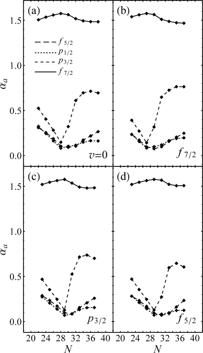
Figure 1: Pair amplitudes $\alpha_{a}$ for the collective $S$-pair (2), as determined variationally by minimization of $E_{\alpha}$ for the various possible minimal-seniority states: (a) the $v=0$ state ($J=0$), for the even-mass $\isotope{Ca}$ isotopes, or the $v=1$ state based upon a quasiparticle in (b) the $f_{7/2}$ orbital ($J=\tfrac{7}{2}$), (c) the $p_{3/2}$ orbital ($J=\tfrac{3}{2}$), or (d) the $f_{5/2}$ orbital ($J=\tfrac{5}{2}$), for the odd-mass $\isotope{Ca}$ isotopes. Calculations are shown for the FPD6 interaction.

The results obtained by the different prescriptions in Fig. 1 are not seen to differ from each other in any substantial qualitative fashion. For the odd-mass $\isotope{Ca}$ isotopes, only the results of calculations carried out using coefficients obtained from the variation involving the $f_{7/2}$ quasiparticle [as in Fig. 1(b)] will be used in the following discussions. The other choices lead to differences in the quantitative details but give similar overall results.

III.2 Energies

Let us begin with the even-mass $\isotope{Ca}$ isotopes, by considering the energy eigenvalue of the $J=0$ ground state, shown in Fig. 2, i.e., the valence shell contribution to the nuclear binding energy. It is worth first noting some properties of the $v=2$ model space for $J=0$. This space is spanned by the four states $|S^{\mathcal{N}-1}A_{{a}{a}}^{0}\rangle$, where $a$ runs over the four $pf$-shell orbitals. However, when the coefficients $\alpha_{a}$ appearing in the $S$ pair are chosen so as to minimize the energy of the $v=0$ condensate state $|S^{\mathcal{N}}\rangle$, as described in Sec. II, the ground state obtained by diagonalization in the $v=2$ space is still simply this condensate (see Appendix). Thus, as far as the ground state is concerned, the $v=2$ results are identical to those for the $v=0$ condensate — or, equivalently, to the results of number-projected BCS, with variation after projection.

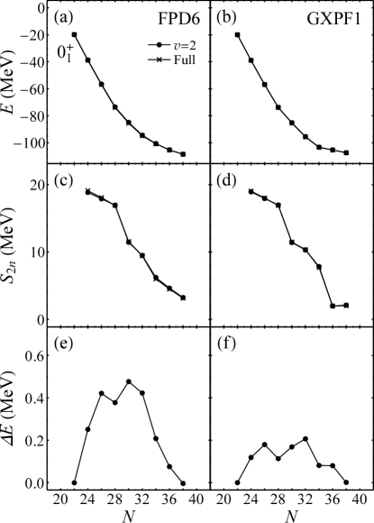
Figure 2: Energy eigenvalue of the $J=0$ ground-state, for the even-mass $\isotope{Ca}$ isotopes, calculated in the generalized seniority $v=2$ model space (circles) or full shell model space (crosses). The energies are considered directly as eigenvalues (top), as two-neutron separation energies $S_{2n}$ (middle), or as the residual difference $\Delta E$ of the generalized seniority result relative to the full shell model result (bottom). Calculations are shown for the FPD6 (left) and GXPF1 (right) interactions.

The ground state energy eigenvalue itself is shown in Fig. 2(a,b), as a function of $N$, for the FPD6 and GXPF1 interactions. The results obtained in the generalized seniority $v=2$ model space and in the full shell model space are overlaid in these plots. However, the deviations are so small that the results are essentially indistinguishable, when viewed on the $\sim 100\,\mathrm{MeV}$ energy scale necessary to accomodate the eigenvalues.

The two-neutron separation energy [$S_{2n}(N)=E(N)-E(N-2)$], shown in Fig. 2(c,d), reveals finer details, in particular differences between the interactions (comparing the two panels), but the generalized seniority and full shell model results are still largely indistinguishable at this scale. A distinctive feature of generalized seniority as an exact symmetry, in the sense of Talmi talmi1971:shell-seniority , is that the ground state energies vary quadratically across the shell, and the separation energies are therefore strictly linear in $N$, insensitive to any subshell closures talmi1975:gssm-mistreatment . However, as observed in Ref. pittel1985:gssm-strong-shell , when generalized seniority is simply used as a variational approach, there is no such constraint, and it is possible to obtain subshell effects. Therefore, it is worth noting the jump in $S_{2n}$ at the $f_{7/2}$ subshell closure ($N=28$) in the generalized seniority calculations [Fig. 2(c,d)], in agreement with the full shell model calculations.

To more clearly compare the calculated ground state energy in the generalized seniority $v=2$ model space with that in the full model space, we consider the residual energy difference $\Delta E$, obtained by subtracting the full space result from the generalized seniority result, shown in Fig. 2(e,f). This difference may be considered as the missing correlation energy, not accounted for in the $S$-pair condensate description of the ground state. By the variational principle, the quantity $\Delta E$ must be nonnegative, since the $v=2$ space is a subspace of the full model space. The residual vanishes where the $v=2$ and full calculations are equivalent, at $N=22$ and $38$ (see Sec. III.1). For the FPD6 interaction [Fig. 2(e)], the residual energy difference grows more or less smoothly towards mid-shell, where it is $0.48\,{\mathrm{MeV}}$. For the GXPF1 interaction [Fig. 2(f)], the residual energy differences are generally smaller by a factor of $\sim 2$, peaking at $0.21\,{\mathrm{MeV}}$. For both interactions, there is a small ($\sim 0.1\,{\mathrm{MeV}}$) dip in the residual at the $f_{7/2}$ subshell closure ($N=28$). This is consistent, albeit not dramatically, with the hypothesis of Ref. monnoye2002:gssm-ni , that the generalized seniority description should improve at subshell closures.

For the energy eigenvalues of the ground state and other low-lying states, the deviations of the generalized seniority $v=2$ model space results from those obtained in the full space are summarized in Table 2. The values given are averages (root-mean-square) of the deviations across the full range of neutron numbers. It may be noted that the deviations are consistently smaller for the GXPF1 interaction than for the FPD6 interaction.

Table 2: Deviations $\Delta E$ (in $\mathrm{MeV}$) between energy eigenvalues calculated in the generalized seniority model space with one broken pair ($v=2$ or $3$) and in the full shell model space. These are root-mean-square averages over the full set of even-mass or odd-mass $\isotope{Ca}$ isotopes with $21\leq N\leq 39$. Values are given for selected states and for the FPD6 and GXPF1 interactions.

$J$	$0^{+}_{1}$	$2^{+}_{1}$	$4^{+}_{1}$	$0^{+}_{2}$	$\tfrac{7}{2}^{-}_{1}$	$\tfrac{5}{2}^{-}_{1}$	$\tfrac{3}{2}^{-}_{1}$	$\tfrac{1}{2}^{-}_{1}$
FPD6	$0.31$	$0.48$	$0.62$	$0.88$	$0.45$	$0.31$	$0.30$	$0.48$
GXPF1	$0.13$	$0.25$	$0.34$	$0.63$	$0.13$	$0.20$	$0.13$	$0.21$

Excitation energies $E_{x}$ for the first $J=2$ and $4$ states, calculated relative to the $J=0$ ground state, are shown in Fig. 3. Although the deviations of $\lesssim 0.5\,{\mathrm{MeV}}$ noted above for the eigenvalues (Table 2) are comparatively small on the $\sim 100\,{\mathrm{MeV}}$ scale of these eigenvalues [Fig. 2(a,b)], they are significant on the few-$\mathrm{MeV}$ scale of the excitation energies. The broad features of the evolution of $E_{x}$ across the shell are reproduced within the $v=2$ model space. For instance, for the $J=2$ state [Fig. 3(a,b)], spikes are obtained at the $f_{7/2}$ subshell closure ($N=28$) and $p_{3/2}$ subshell closure ($N=32$ for FPD6 or $\sim 32$–$34$ for GXPF1). Quantitatively, the excitation energy calculated for the $J=2$ state deviates from that calculated in the full model space by at most $0.41\,{\mathrm{MeV}}$ for FPD6 or $0.23\,{\mathrm{MeV}}$ for GXPF1. For the $J=4$ state, the largest deviations obtained are $0.58\,{\mathrm{MeV}}$ for FPD6 or $0.53\,{\mathrm{MeV}}$ for GXPF1. For both states, the excitation energies calculated in the $v=2$ model space are systematically higher than those calculated in the full model space, even though this direction for the deviation is not guaranteed by any variational principle.

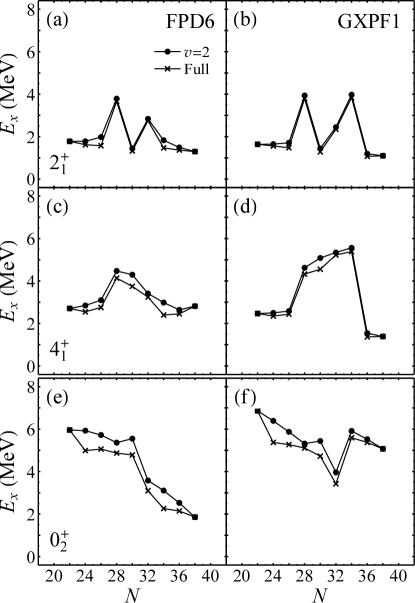
Figure 3: Excitation energies $E_{x}$ of the lowest $J=2$ state (top), lowest $J=4$ state (middle), and first excited $J=0$ state (bottom) of the even-mass $\isotope{Ca}$ isotopes, calculated in the generalized seniority $v=2$ model space (circles) or full shell model space (crosses). Calculations are shown for the FPD6 (left) and GXPF1 (right) interactions.

Returning to the $J=0$ states, the question arises as to whether or not the first excited $J=0$ state can be reasonably reproduced within the $v=2$ space. The calculated excitation energy for this state is shown in Fig. 3(e,f). The general expectation bonsignori1985:bpm-sn is that $v=4$ or higher contributions should be important for an accurate description. The description of the excitation energy [Fig. 3(e,f)] within the $v=2$ model space is qualitatively reasonable, but it is also quantitatively less accurate than for the yrast states (see Table 2). The calculation within the $v=2$ model space reproduces the main features of the $N$ dependence of the first excited $J=0$ energy: roughly constant $E_{x}\sim 5\,{\mathrm{MeV}}$ for $N\leq 30$, followed by a drop to $E_{x}\sim 3\,{\mathrm{MeV}}$ at $N=32$ for the FPD6 interaction [Fig. 3(e)], or a transient dip in the case of the GXPF1 interaction [Fig. 3(f)]. The largest deviation is $\lesssim 1\,{\mathrm{MeV}}$. However, from the occupations (Sec. III.3), it will be seen that physically significant differences arise between the nature of the excited $J=0$ state obtained in the $v=2$ model space and in the full model space, in the lower part of the shell. The excitation energy is, once again, systematically calculated higher in the generalized seniority model space than in the full model space.

For the odd-mass $\isotope{Ca}$ isotopes, the level energies calculated in the generalized seniority $v=1$ and $v=3$ model spaces are shown in Fig. 4. Let us begin by examining the energy eigenvalue for the lowest $J=\tfrac{7}{2}$ state [Fig. 4(a,b)]. This is the ground state (both calculated and experimental) for $21\leq N\leq 27$, where nucleons in the $f_{7/2}$ subshell dominate the structure. The $v=1$ calculation constitutes the most extreme approximation within the generalized seniority framework — attempting to treat the lowest-energy state as a one-quasiparticle state based upon the $f_{7/2}$ orbital. It is seen that the energy obtained in the $v=1$ calculation differs from that is the full space very noticeably (several $\mathrm{MeV}$) for a range of $N$ values above the $f_{7/2}$ subshell closure ($N\geq 31$ for FPD6 [Fig. 4(a)] or $N\geq 35$ for FPD6 [Fig. 4(b)]). The energy obtained in the $v=3$ space, however, is indistinguishable from the result in the full space, on this scale. We therefore again consider residual energy differences [Fig. 4(c,d)]. Similar comments apply to the energies of the lowest states of $J=\tfrac{5}{2}$, $\tfrac{3}{2}$, and $\tfrac{1}{2}$, calculated in the $v=1$ and $v=3$ model spaces, for which the residuals are shown in Fig. 4(e–j), although the range of $N$ under which the $v=1$ approximation deviates most differs for the different states. For all states, the residual energy difference for the $v=3$ calculation identically vanishes at $N=23$ and $37$, where the $v=3$ and full calculations are equivalent, and similarly for the $v=1$ calculation at $N=21$ and $39$.

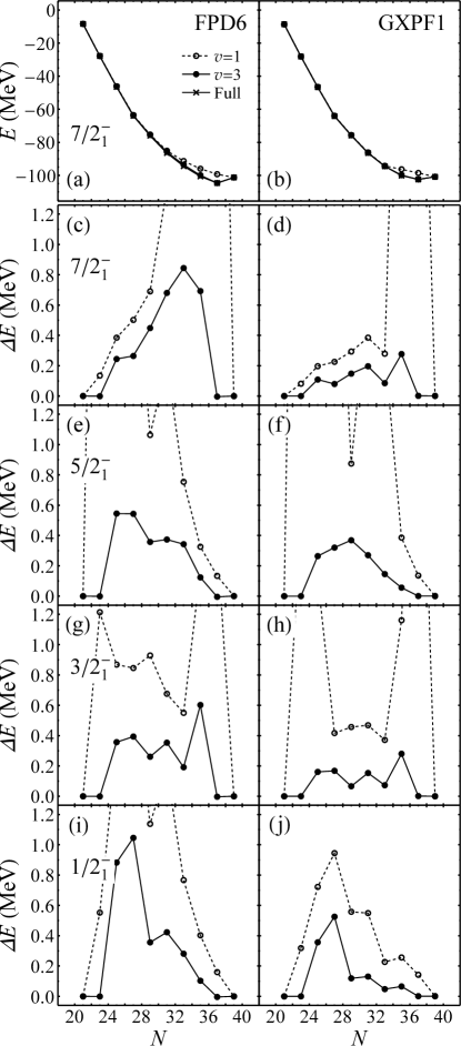
Figure 4: (a–b) Energy eigenvalue of the lowest $J=\tfrac{7}{2}$ state, for the odd-mass $\isotope{Ca}$ isotopes, calculated in the generalized seniority $v=1$ model space (open circles), generalized seniority $v=3$ model space (filled circles), or full shell model space (crosses). (c–j) Residual differences $\Delta E$ of the generalized seniority result relative to the full shell model result, for the energy eigenvalues of the lowest $J=\tfrac{7}{2}$, $\tfrac{5}{2}$, $\tfrac{3}{2}$, and $\tfrac{1}{2}$ states (top to bottom, respectively). Calculations are shown for the FPD6 (left) and GXPF1 (right) interactions.

The differences between energies calculated in the $v=3$ space and the full shell model space are again typically smaller for the GXPF1 interaction than for the FPD6 interaction. For the $J=\tfrac{7}{2}$ state, the residual reaches $0.84\,{\mathrm{MeV}}$ for the FPD6 interaction [Fig. 4(c)] but is never larger than $0.28\,{\mathrm{MeV}}$ for the GXPF1 interaction [Fig. 4(d)]. Given the sharp $N$ dependences observed in Fig. 4, global averages of the deviations across the shell provide only a very crude measure of the level of agreement between $v=3$ and full space calculations. Nonetheless, the quantitative results are summarized in Table 2.

The range of neutron numbers over which the $v=1$ approximation provides a reasonable reproduction of the full space results, for each different $J$, can be roughly interpreted in terms of the natural filling order of the orbitals (see also the discussion of occupations below in Sec. III.3). First, it should be noted that, although the $v=1$ state $|S^{\mathcal{N}}C_{a}\rangle$ involves a superposition of different possible occupation numbers for the orbital $a$, since the $S^{\dagger}$ operator adds particles in pairs to each orbital, the state will involve contributions only with an odd occupation for the orbital $a$. The one-quasiparticle description therefore requires at least one particle in the given orbital $a$, but also at least one hole in that orbital.

For instance, for the $J=\tfrac{7}{2}$ state to be one-quasiparticle in nature requires the presence of at least one particle but also one hole in the $f_{7/2}$ orbital. This is naturally the situation early in the shell, but retaining a vacancy in the $f_{7/2}$ orbital becomes increasingly energetically penalized as the shell fills. Once more nucleons are present than can be accomodated in the $f_{7/2}$ orbital, the one-quasiparticle state is subject to the single-particle energy cost of promoting at least one nucleon out of the $f_{7/2}$ orbital, to leave an $f_{7/2}$ hole. It would thus be natural to expect the one-quasiparticle state to lie several $\mathrm{MeV}$ higher in energy than other configurations. The residual energy difference between the one-quasiparticle state and the lowest $J=\tfrac{7}{2}$ state in the full space does indeed jump to several $\mathrm{MeV}$ after the $f_{7/2}$ subshell closure [Fig. 4(d)], but only at neutron numbers somewhat larger than $N=28$. This may be understood in terms of the impossibility of generating $J=\tfrac{7}{2}$ with nucleons purely in the next available orbital, $p_{3/2}$. The configurations competing with the one-quasiparticle state therefore are also subject to a single-particle energy penalty for promoting nucleons to yet higher orbitals (see Sec. III.3 for the orbitals actually involved).

Similar interpretations may be given for the $v=1$ energies for the other $J$ values. For the $J=\tfrac{5}{2}$ state to be one-quasiparticle in nature requires at least one particle in the $f_{5/2}$ orbital. Since the $f_{5/2}$ orbital is highest in the shell, configurations involving a particle in this orbital only become favored by single-particle energy considerations above $N\approx 34$. For both interactions, the $v=1$ energy residual is indeed lowest at the very end of the shell [Fig. 4(g,h)], dropping below $\sim 0.5\,{\mathrm{MeV}}$ for $N\geq 35$. For the $J=\tfrac{3}{2}$ state, natural filling of the $p_{3/2}$ orbital occurs midshell, for $29\leq N\leq 31$. The $v=1$ energy residual for the $J=\tfrac{3}{2}$ state is lowest in this mid-shell region, although the reduction is not sharply confined to these particular neutron numbers [Fig. 4(k,l)]. For the $J=\tfrac{1}{2}$ state, the interpretation of the $v=1$ energy residual [Fig. 4(k,l)] is less clear. Natural filling would occur in a very limited region just above midshell ($N\approx 33$). On the other hand, it is also relatively difficult to generate energetically favored shell model configurations with $J=1/2$ to compete with the one-quasiparticle configuration. For instance, at the beginning of the shell, no pure $f_{7/2}^{n}$ configuration has $J=\tfrac{1}{2}$, so any competing configuration in the full model space will likewise involve promoting at least one particle out of the $f_{7/2}$ subshell.

III.3 Occupations

The occupations of the $pf$-shell orbitals provide a simple, direct measure of the structure of the shell model eigenstates. The occupations may also be considered as experimental observables, through their connection to spectroscopic factors.

Table 3: Deviations between orbital occupations $\langle n_{a}\rangle$ calculated in the generalized seniority model space with one broken pair ($v=2$ or $3$) and in the full shell model space. These are root-mean-square averages over the full set of even-mass or odd-mass $\isotope{Ca}$ isotopes with $21\leq N\leq 39$, taking all four $pf$-shell orbitals into account. Values are given for selected states and for the FPD6 and GXPF1 interactions.

$J$	$0^{+}_{1}$	$2^{+}_{1}$	$4^{+}_{1}$	$0^{+}_{2}$	$\tfrac{7}{2}^{-}_{1}$	$\tfrac{5}{2}^{-}_{1}$	$\tfrac{3}{2}^{-}_{1}$	$\tfrac{1}{2}^{-}_{1}$
FPD6	$0.03$	$0.09$	$0.11$	$0.29$	$0.06$	$0.04$	$0.05$	$0.09$
GXPF1	$0.015$	$0.03$	$0.08$	$0.26$	$0.015$	$0.03$	$0.02$	$0.14$

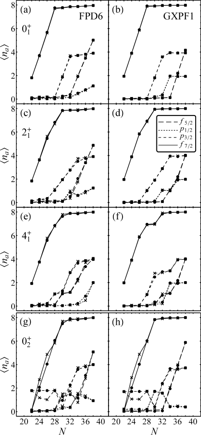
Figure 5: Orbital occupations $\langle n_{a}\rangle$ of the $pf$-shell orbitals, for the lowest $J=0$, $2$, and $4$ states and first excited $J=0$ state (top to bottom, respectively) of the even-mass $\isotope{Ca}$ isotopes, calculated in the generalized seniority $v=2$ model space (circles) or full shell model space (crosses). Calculations are shown for the FPD6 (left) and GXPF1 (right) interactions.

While the basis states used in traditional shell model calculations have a definite number of nucleons in each orbital, by construction, the generalized seniority basis states do not. Indeed, the $S$-pair condensate has a BCS-like distribution of occupations for the different orbitals. Nonetheless, the orbital occupations for states obtained in the generalized seniority scheme can readily be calculated much as any other one-body observable (Sec. II), as the expectation values $\langle n_{a}\rangle$.

The orbital occupations for the even-mass $\isotope{Ca}$ isotopes are shown in Fig. 5, for the same states as considered in Sec. III.2, calculated both in the generalized seniority $v=2$ model space and in the full shell model space. For the lowest $J=0$, $2$, and $4$ states [Fig. 5(a–f)], the curves obtained in the $v=2$ and full spaces are nearly indistinguishable. For the ground state in particular (recall the $v=2$ ground state is just the $S$-pair condensate), the generalized seniority approximation reproduces the mean occupation to within $0.1$ nucleon for all the orbitals, across the entire shell. The typical deviations in $\langle n_{a}\rangle$ for the ground state are in fact even much smaller, $\sim 0.03$ for the FPD6 interaction or $\sim 0.015$ for the GXPF1 interaction. The deviations are only modestly larger for the $J=2$ and $4$ states, as summarized in Table 3. Qualitatively, the trend appears to be that the generalized seniority calculations smooth the evolution of the occupations as functions of $N$, relative to the calculations in the full space. Such is observed if one examines the difference between the curves obtained in the $v=2$ and full spaces for the occupations of, for instance, the $p_{3/2}$ or $f_{5/2}$ orbitals at $N=34$ for the $J=2$ state, under FPD6 [Fig. 5(c)], or for the $p_{3/2}$ orbital at $N=30$ for the $J=4$ state, under either interaction [Fig. 5(e,f)].

Inspection of the occupations for the ground state and excited $J=2$ state below the $f_{7/2}$ subshell closure ($N=28$) in Fig. 5(a–d) indicates that these are nearly pure $f_{7/2}^{n}$ configurations, with just trace occupations of the other $pf$-shell orbitals. In the limit of a pure $f_{7/2}^{n}$ configuration, the generalized seniority description reduces to the conventional seniority description in the $f_{7/2}$ shell, indeed, a classic domain for application of seniority suhonen2007:nucleons-nucleus . That is, the generalized seniority $v=0$ state is just the conventional zero-seniority state, the generalized seniority $v=2$ space contains just the conventional seniority $2$ state of each $J$, etc. Generalized seniority thus only becomes fully distinct from conventional seniority when multiple orbitals are simultaneously significantly occupied, above $N=28$.

The calculated occupations for the first excited $J=0$ state are shown in Fig. 5(e,f). As already noted in Sec. III.2, the generalized seniority $v=2$ calculation is taking place in a very low-dimensional space. The $v=2$ results are seen to track those obtained in the full space reasonably well across the shell, but with notable differences below the $f_{7/2}$ subshell closure ($N=28$). In particular, these indicate differing structural interpretations for the excited state in the $v=2$ model space and the full space in the lower part of the shell. In the $v=2$ space for $J=0$, the nucleons must couple to zero angular momentum pairwise (recall the $|S^{\mathcal{N}-1}A_{{a}{a}}^{0}\rangle$ basis states) and thus occupy orbitals in even numbers. Therefore, a $f_{7/2}^{n-2}p_{3/2}^{2}$ excited state is obtained at $N=24$ and $26$ [see the $p_{3/2}$ curve for $v=2$ in Fig. 5(e,f)], as the next most energetically favored configuration after the approximately-$f_{7/2}^{n}$ ground state. However, the structure in the full model space is found to involve promotion of only a single nucleon to the $p_{3/2}$ orbital [see the $p_{3/2}$ curve for the full space calculation in Fig. 5(e,f)]. The remaining nucleons in the $f_{7/2}$ orbital must therefore be in a $J=\tfrac{3}{2}$ configuration, which has conventional seniority $3$, so that total $J=0$ may be obtained. However, above the $f_{7/2}$ subshell closure, agreement of the occupations in the $v=2$ and full spaces is much closer.

The occupations of the orbitals in the odd-mass $\isotope{Ca}$ isotopes are shown in Fig. 6, as calculated in the generalized seniority $v=3$ model space and the full shell model space. The lowest $J=\tfrac{7}{2}$ and $\tfrac{5}{2}$ states are taken for illustration. The results obtained in the generalized seniority $v=3$ model space again closely track those found in the full model space. The quantitative deviations are again summarized in Table 3, and again those for the GXPF1 interaction are smaller than for the FPD6 interaction.

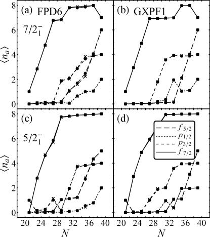
Figure 6: Orbital occupations $\langle n_{a}\rangle$ of the $pf$-shell orbitals, for the lowest $J=\tfrac{7}{2}$ (top) and $J=\tfrac{5}{2}$ (bottom) states of the odd-mass $\isotope{Ca}$ isotopes, calculated in the generalized seniority $v=3$ model space (circles) or full shell model space (crosses). Calculations are shown for the FPD6 (left) and GXPF1 (right) interactions.

As discussed in Sec. III.2, the $v=1$ one-quasiparticle description varies greatly with $N$ in its success at reproducing the energy of the lowest state of each $J$, and this variation may qualitatively be interpreted in terms of the single particle energy cost of generating a quasiparticle in the relevant orbital. The orbital occupations in Fig. 6 provide an immediate indication of whether or not a given state might be dominantly one-quasiparticle in nature, if we recall that the orbital containing the quasiparticle must have odd occupation, and therefore contain at least one particle but also one hole. For instance, for the $J=\tfrac{7}{2}$ state, recall that the $v=1$ result provides a reasonable description of the energy only for $N\leq 29$ for the FPD6 interaction [Fig. 4(c)] or for $N\leq 33$ for the GXPF1 interaction [Fig. 4(d)]. Examining the occupation of the $f_{7/2}$ orbital in the $J=\tfrac{7}{2}$ state [Fig. 6(a,b)], it is seen that, indeed, the occupation is only consistent with an $f_{7/2}$ quasiparticle for $N\leq 29$ for the FPD6 interaction [Fig. 6(a)], after which the $f_{7/2}$ orbital completely fills, but that a hole remains in the $f_{7/2}$ orbital for $N\leq 33$ for the GXPF1 interaction [Fig. 6(b)]. For the $J=\tfrac{5}{2}$ state [Fig. 6(c,d)], the situation is less obvious. The calculated occupations admit the possibility of one-quasiparticle structure for $N\geq 29$ for FPD6 [Fig. 6(c)] or $N\geq 33$ for FPD6 [Fig. 6(c)], since these are the ranges over which the $f_{5/2}$ orbital has an occupation of at least one, but recall that the $v=1$ calculation provides a reasonable description of the energy only for $N\gtrsim 35$ [Fig. 4(g,h)]. One may also directly examine the occupations obtained in the $v=1$ calculations (not shown in Fig. 6), and they are found to track the results from the full space calculations very well over the ranges of $N$ just described and poorly outside of these ranges.

III.4 Electromagnetic observables

The matrix elements of electromagnetic transition operators (which we will consider in spectroscopic terms, as electromagnetic moments or transition strengths) probe the extent to which various correlations are preserved when the nuclear calculation is carried out in a space of restricted generalized seniority. Practically, the accuracy with which these observables are reproduced is of prime interest if generalized seniority is to be used as a truncation scheme for shell model calculations.

Matrix elements of the $E2$ and $M1$ operators directly follow from the one-body densities calculated in the generalized seniority scheme (Sec. II) much as in a conventional shell model calculation. It should be noted that the FPD6 and GXPF1 interactions are defined only in terms of two-body matrix elements between orbitals labeled by quantum numbers $nlj$, without reference to any specific form for the radial wave functions. A particular choice must be made if electromagnetic transition observables are to be computed. We adopt harmonic oscillator wave functions, with the Blomqvist-Molinari parametrization $\hbar\omega=(45\,{\mathrm{MeV}})A^{-1/3}-(25\,{\mathrm{MeV}})A^{-2/3}$ suhonen2007:nucleons-nucleus for the oscillator energy. Since only neutrons are present for the $\isotope{Ca}$ isotopes, the overall normalization of the $E2$ matrix elements is set by the neutron effective charge, which is taken as $e_{\nu}=0.5$. For the calculation of $M1$ matrix elements, the free-space neutron $g$-factors are used.

For the even-mass $\isotope{Ca}$ isotopes, we consider the electric quadrupole moment $Q(2^{+}_{1})$, electric quadrupole reduced transition probability $B(E2;2^{+}_{1}\rightarrow 0^{+}_{1})$, and magnetic dipole moment $\mu(2^{+}_{1})$, as representative electromagnetic observables for the low-lying states. The values are shown in Fig. 7, calculated both in the $v=2$ and full shell model spaces.

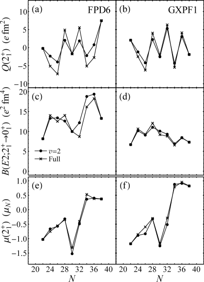
Figure 7: Electromagnetic observables for the even-mass $\isotope{Ca}$ isotopes: $Q(2^{+}_{1})$ (top), $B(E2;2^{+}_{1}\rightarrow 0^{+}_{1})$ (middle), and $\mu(2^{+}_{1})$ (bottom), calculated in the generalized seniority $v=2$ model space (circles) or full shell model space (crosses). Calculations are shown for the FPD6 (left) and GXPF1 (right) interactions.

For the quadrupole moment [Fig. 7(a,b)], the calculation in the $v=2$ space qualitatively tracks the results for the full space, in particular, the alternations in sign as a function of neutron number. However, under the FPD6 interaction [Fig. 7(a)], the quadrupole moment obtained in the $v=2$ space is consistently much smaller in magnitude than in the full space, roughly by a factor of two. The difference under the GXPF1 interaction [Fig. 7(b)] is less marked, but the quantitative agreement is still crude. The quadrupole moment obtained in the $v=2$ space is smaller by $\sim 30\%$, that is the average deviation from the full-space result is $1.2\,e\mathrm{fm}^{2}$ (taking root-mean-square averages to better accomodate signed quantities), on quadruople moments averaging $4\,e\mathrm{fm}^{2}$. This attenuation of the calculated quadrupole moment is perhaps not surprising, given that the generalized seniority scheme is expected to be restricted in its ability to reproduce quadrupole correlations talmi1983:ibm-shell .

However, for the $B(E2;2^{+}_{1}\rightarrow 0^{+}_{1})$ strength [Fig. 7(c,d)], which is often taken as a proxy for the quadrupole deformation, the agreement between the values obtained in the $v=2$ model space and in the full shell model space is much closer than for $Q(2^{+}_{1})$. Here the deviations under FPD6 are $\sim 12\%$ [averaging $1.6\,e^{2}\mathrm{fm}^{4}$, on $B(E2)$ values averaging $13\,e^{2}\mathrm{fm}^{4}$], or for GXPF1 only $\sim 6\%$ [averaging $0.5\,e^{2}\mathrm{fm}^{4}$, on $B(E2)$ values averaging $9\,e^{2}\mathrm{fm}^{4}$]. Thus, intriguingly, generalized seniority seems more capable of incorporating the correlations necessary for reproducing $B(E2;2^{+}_{1}\rightarrow 0^{+}_{1})$ than for reproducing $Q(2^{+}_{1})$.

The magnetic dipole moment of the first $J=2$ state [Fig. 7(e,f)] evolves in a complicated manner with neutron number, involving multiple reversals in sign, and these are well reproduced by the calculations in the generalized seniority $v=2$ model space. (The most noticeable discrepancy arises for the GXPF1 interaction at $N=26$ [Fig. 7(f)], also the point of largest deviation in the $2^{+}$ excitation energy [Fig. 3(b)] for this interaction, but unremarkable in terms of occupations [Fig. 5(d)].) Quantitatively, the deviations are comparable for both interactions, for FPD6 $\sim 14\%$ (averaging $0.10\mu_{N}$, on moments averaging $0.7\mu_{N}$) or for GXPF1 $\sim 15\%$ (averaging $0.12\mu_{N}$, on moments averaging $0.8\mu_{N}$).

For the odd-mass $\isotope{Ca}$ isotopes, let us consider the electromagnetic moments $Q(\tfrac{7}{2}^{-}_{1})$ and $\mu(\tfrac{7}{2}^{-}_{1})$ of the first $J=\tfrac{7}{2}$ state. The values are shown in Fig. 8, calculated in the generalized seniority $v=1$ and $v=3$ model spaces and in the full shell model space. For both these moments, the evolution calculated in the $v=3$ model space closely tracks that obtained in the full model space, with isolated discrepancies. For the quadrupole moment [Fig. 8(a,b)], the deviations for FPD6 are $\sim 15\%$ (averaging $0.9\,e\mathrm{fm}^{2}$, on moments averaging $6\,e\mathrm{fm}^{2}$) or for GXPF1 $\sim 4\%$ (averaging $0.19\,e\mathrm{fm}^{2}$, on moments averaging $5\,e\mathrm{fm}^{2}$). Notice the much better agreement obtained for this quadrupole moment in the $v=3$ space than for $Q(2^{+}_{1})$ in the $v=2$ space. For the dipole moment [Fig. 8(c,d)], the deviations for FPD6 are $\sim 14\%$ (averaging $0.19\,e\mathrm{fm}^{2}$, on moments averaging $1.4\,e\mathrm{fm}^{2}$) or for GXPF1 $\sim 3\%$ (averaging $0.05\,e\mathrm{fm}^{2}$, on moments averaging $1.5\,e\mathrm{fm}^{2}$).

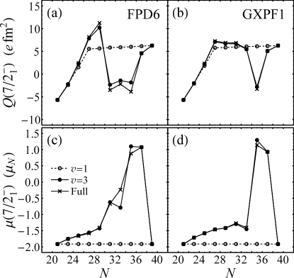
Figure 8: Electromagnetic observables for the odd-mass $\isotope{Ca}$ isotopes: $Q(\tfrac{7}{2}^{-}_{1})$ (top) and $\mu(\tfrac{7}{2}^{-}_{1})$ (bottom), calculated in the generalized seniority $v=1$ model space (open circles), generalized seniority $v=3$ model space (filled circles), or full shell model space (crosses). Calculations are shown for the FPD6 (left) and GXPF1 (right) interactions.

The quadrupole moment $Q(\tfrac{7}{2}^{-}_{1})$ obtained in the one-quasiparticle ($v=1$) description [Fig. 8(a,b)] can be understood in terms of the single particle value for the $f_{7/2}$ orbital and conventional seniority arguments. For the one-quasiparticle state $|S^{\mathcal{N}}C_{a}\rangle$, only the orbital $a$ can contribute to the quadrupole moment (simply by angular momentum selection), and this orbital carries a conventional seniority of $1$ from the unpaired particle. Conventional seniority in a $j^{n}$ configuration gives a simple linear variation of the quadrupole moment with $n$ across the $j$-shell, vanishing midshell (the quadrupole operator is part of a rank-$1$ tensor with respect to quasispin macfarlane1966:shell-identical ). This conventional seniority result cannot be directly applied to the generalized seniority one-quasiparticle state, unless the occupation $n_{a}$ is approximately sharp in this state. Recall that this is indeed the case for the $f_{7/2}$ orbital, under the present interactions, where the occupations below $N=28$ are, to very good approximation, $n_{7/2}=N-20$ [Fig. 6(a,b)]. Thus, across the $f_{7/2}$ subshell, the quadrupole moment for the $J=\tfrac{7}{2}$, $v=1$ state [Fig. 8(a,b)] varies linearly from the $f_{7/2}$ single-particle value to the $f_{7/2}$ single-hole value. Then, above the subshell closure, the $v=1$ state has, to very good approximation, $n_{7/2}=7$, i.e., exactly one hole. Thus, the $v=1$ quadrupole moment plateaus at the $f_{7/2}$ single-hole value. The range of neutron numbers over which the one-quasiparticle calculation provides a reasonable approximation to the quadrupole moment is $N\leq 25$ for the FPD6 interaction or $N\leq 35$ for the GXPF1 interaction, and again for $N\geq 37$. This does not quite correspond to the ranges found in Secs. III.2 and III.3 from energies and occupations, i.e., $N\leq 29$ for the FPD6 interaction or $N\leq 33$ for the GXPF1 interaction.

The dipole moment $\mu(\tfrac{7}{2}^{-}_{1})$ obtained in the one-quasiparticle description [Fig. 8(c,d)] is, more simply, constant (the dipole operator is scalar with respect to quasispin macfarlane1966:shell-identical ) and has the single-particle Schmidt value. The departure of the full space result from the Schmidt value is modest over the range $N\leq 29$ for the FPD6 interaction or $N\leq 33$ for the GXPF1 interaction, and consists of a smooth linear evolution with $N$ (increasing from $-1.91\mu_{N}$ to $\sim-1.5\mu_{N}$), before jumping abruptly at the ends of these ranges. This may be interpreted as reflecting the same one-quasiparticle nature observed in the energies (Secs. III.2) and occupations (Sec. III.3) over these ranges.

IV Conclusions

From the comparisons carried out in this work, it is found that calculations in a highly-truncated, low-dimensional (Table 1) generalized seniority model space, with just one broken pair, can reproduce energy, occupation, and electromagnetic observables for low-lying states with varying — but in some cases remarkably high — fidelity to the results obtained in the full shell model space. These results were obtained for semimagic nuclei in the $pf$ shell, under two different realistic interactions. Deviations in energies (Table 2) vary from the $\sim 150\,{\mathrm{keV}}$ range to the $1\,{\mathrm{MeV}}$ range for the states considered, which, while small compared to the $100\,{\mathrm{MeV}}$ binding energies, is nonnegligible for the evaluation of few-${\mathrm{MeV}}$ excitation energies. Nonetheless, the evolution of excitation energies is reasonably well-reproduced across the shell. For level occupations of the low-lying states (Table 3), accuracies in the few-percent range are obtained. With the notable exception of $Q(2^{+}_{1})$ in the even-mass nuclei, electric quadrupole and magnetic dipole observables are reproduced to $\sim 10\%$ or better (Sec. III.4). Given the distinct improvement of results from the $v=1$ space to the $v=3$ space (for the odd-mass nuclei), the most natural extension is to generalized seniority spaces with two broken pairs ($v=4$ for even-mass nuclei and $5$ for odd-mass nuclei).

Aside from the conceptual interest of generalized seniority as a means of interpreting shell model results in a BCS pair-condensate plus quasiparticle framework, real computational benefits will be obtained if generalized seniority can also be successfully applied as an accurate truncation scheme for nuclei in the interior of the shell, when significant numbers of both valence protons and neutrons are present. The obvious challenge is the seniority-nonconserving, or pair-breaking, nature of the proton-neutron interaction talmi1983:ibm-shell , since a pair broken in the conventional seniority scheme also implies breaking of a generalized seniority $S$ pair. The approach is likely to be more advantageous for weakly-deformed nuclei (in large model spaces) than for strongly-deformed nuclei. Seniority decompositions of shell model calculations caurier2005:shell ; menendez2011:shell-0nu2beta suggest seniorities $\lesssim 8$ should be sufficient for a variety of weakly-deformed nuclei. Such values are consistent with the possibility of successful calculation in a generalized seniority model space with two broken pairs for both protons and neutrons.

It was systematically observed that the calculations in the generalized seniority model space more accurately match those in the full model space for the GXPF1 interaction than for the FPD6 interaction, typically by a factor of $\sim 2$. It would be valuable to have a systematic quantitative understanding of the deviations expected for a given interaction, given some appropriate quantitative measures characterizing the interaction. The question has been addressed in the context of random two-body interactions, in terms of the random ensemble parameters johnson1999:gssm-random ; lei2011:gssm-random . In particular, it appears to be important that the energy spacing scale of the single particle energies be large compared to the scale of the two-body matrix elements lei2011:gssm-random . It might therefore be relevant that the spread of the single particle energies is indeed slightly larger for GXPF1 than for FPD6. Alternatively, since the generalized seniority approach is based upon the dominance of pairing correlations, it is worth investigating the possibility that the decomposition of realistic interactions into pairing and non-pairing (e.g., quadrupole) components through the use of spectral distribution theory, as carried out in Ref. sviratcheva2006:realistic-symmetries , could yield relevant measures.

Appendix

In this appendix, a simple demonstration is provided to establish the property noted in Sec. III.2, that the $J=0$ ground state obtained in the $v=2$ model space is simply the $v=0$ condensate state, provided the $\alpha_{a}$ coefficients have been chosen according to the variational prescription described in Sec. II. It is convenient to first modify the normalization convention on the $\alpha_{a}$ coefficients, from that given in Sec. III.1, so as to instead give the state $|S^{\mathcal{N}}\rangle$ unit normalization. Then the energy functional in the variational prescription simplifies to $E_{\alpha}=\langle{S^{\mathcal{N}}}|{H}|{S^{\mathcal{N}}}\rangle$ and is subject to the constraint $\langle S^{\mathcal{N}}|S^{\mathcal{N}}\rangle=1$. Since $(\partial/\partial\alpha_{a})|S^{\mathcal{N}}\rangle=\mathcal{N}\hat{\jmath}_{a}|S^{\mathcal{N}-1}A_{{a}{a}}^{0}\rangle$, the Lagrange equations for the extremization problem are of the form $\langle{S^{\mathcal{N}-1}A_{{a}{a}}^{0}}|{H}|{S^{\mathcal{N}}}\rangle-\lambda\langle S^{\mathcal{N}-1}A_{{a}{a}}^{0}|S^{\mathcal{N}}\rangle=0$, with a separate equation obtained for each orbital $a$. Since the states $|S^{\mathcal{N}-1}A_{{a}{a}}^{0}\rangle$ span the $v=2$ space, this is simply the condition that $H|S^{\mathcal{N}}\rangle=\lambda|S^{\mathcal{N}}\rangle$ within the $v=2$ space. That is, $|S^{\mathcal{N}}\rangle$ is an eigenstate of the Hamiltonian, and, in practice, it is the ground state. Note that this result also establishes the equivalence of the “iterative diagonalization” prescription for determining the $\alpha_{a}$ coefficients, proposed in Ref. scholten1983:ibm2-microscopic-majorana , to the variational prescription, since the iterative diagonalization prescription determines the $\alpha_{a}$ coefficients so as to decouple the $S$ condensate from the rest of the $v=2$ space, exactly as found above for the variational prescription.

References

- (1) I. Talmi, Nucl. Phys. A 172, 1 (1971).
- (2) S. Shlomo and I. Talmi, Nucl. Phys. A 198, 81 (1972).
- (3) Y. K. Gambhir, A. Rimini, and T. Weber, Phys. Rev. 188, 1573 (1969).
- (4) K. Allaart, E. Boeker, G. Bonsignori, M. Savoia, and Y. K. Gambhir, Phys. Rep. 169, 209 (1988).
- (5) T. Otsuka, A. Arima, and F. Iachello, Nucl. Phys. A 309, 1 (1978).
- (6) F. Iachello and I. Talmi, Rev. Mod. Phys. 59, 339 (1987).
- (7) G. Racah, Phys. Rev. 76, 1352 (1949).
- (8) A. de-Shalit and I. Talmi, Nuclear Shell Theory, Pure and Applied Physics No. 14 (Academic, New York, 1963).
- (9) M. H. Macfarlane, in Lectures in Theoretical Physics, edited by P. D. Kunz, D. A. Lind, and W. E. Britten (The University of Colorado Press, Boulder, 1966), Vol. VIII C, p. 583.
- (10) Y. K. Gambhir, A. Rimini, and T. Weber, Phys. Rev. C 3, 1965 (1971).
- (11) G. Bonsignori and M. Savoia, Nuovo Cimento A 44, 121 (1978).
- (12) S. Pittel, P. D. Duval, and B. R. Barrett, Ann. Phys. (N.Y.) 144, 168 (1982).
- (13) O. Scholten and H. Kruse, Phys. Lett. B 125, 113 (1983).
- (14) G. Bonsignori, M. Savoia, K. Allaart, A. van Egmond, and G. te Velde, Nucl. Phys. A 432, 389 (1985).
- (15) P. Van Isacker, S. Pittel, A. Frank, and P. D. Duval, Nucl. Phys. A 451, 202 (1986).
- (16) P. Navrátil and J. Dobeš, Phys. Rev. C 37, 2126 (1988).
- (17) J. Engel, P. Vogel, X. Ji, and S. Pittel, Phys. Lett. B 225, 5 (1989).
- (18) P. O. Lipas, M. Koskinen, H. Harter, R. Nojarov, and A. Faessler, Nucl. Phys. A 509, 509 (1990).
- (19) T. Otsuka, Prog. Theor. Phys. Suppl. 125, 5 (1996).
- (20) N. Yoshinaga, T. Mizusaki, A. Arima, and Y. D. Devi, Prog. Theor. Phys. Suppl. 125, 65 (1996).
- (21) O. Monnoye, S. Pittel, J. Engel, J. R. Bennett, and P. Van Isacker, Phys. Rev. C 65, 044322 (2002).
- (22) J. Barea and F. Iachello, Phys. Rev. C 79, 044301 (2009).
- (23) N. Sandulescu, J. Blomqvist, T. Engeland, M. Hjorth-Jensen, A. Holt, R. J. Liotta, and E. Osnes, Phys. Rev. C 55, 2708 (1997).
- (24) Y. Lei, Z. Y. Xu, Y. M. Zhao, and A. Arima, Phys. Rev. C 82, 034303 (2010).
- (25) W. A. Richter, M. G. van der Merwe, R. E. Julies, and B. A. Brown, Nucl. Phys. A 523, 325 (1991).
- (26) M. Honma, T. Otsuka, B. A. Brown, and T. Mizusaki, Phys. Rev. C 69, 034335 (2004).
- (27) B. A. Brown, Prog. Part. Nucl. Phys. 47, 517 (2001).
- (28) E. Caurier, G. Martínez-Pinedo, F. Nowacki, A. Poves, and A. P. Zuker, Rev. Mod. Phys. 77, 427 (2005).
- (29) I. Talmi, Prog. Part. Nucl. Phys. 9, 27 (1983).
- (30) A. Frank and P. Van Isacker, Phys. Rev. C 26, 1661 (1982).
- (31) F. Q. Luo and M. A. Caprio, Nucl. Phys. A 849, 35 (2011).
- (32) J. Suhonen, From Nucleons to Nucleus (Springer-Verlag, Berlin, 2007).
- (33) T. Mizusaki and T. Ostuka, Prog. Theor. Phys. Suppl. 125, 97 (1996).
- (34) T. Otsuka, Nucl. Phys. A 557, 531c (1993).
- (35) W. D. M. Rae, computer code NuShellX (unpublished); B. A. Brown, W. D. M. Rae, E. McDonald, and M. Horoi, computer code NuShellX@MSU (unpublished).
- (36) I. Talmi, Phys. Lett. B 55, 255 (1975).
- (37) S. Pittel, O. Scholten, and T. Otsuka, Phys. Lett. B 157, 239 (1985).
- (38) J. Menéndez, A. Poves, E. Caurier, and F. Nowacki, J. Phys. Conf. Ser. 267, 012058 (2011).
- (39) C. W. Johnson, G. F. Bertsch, D. J. Dean, and I. Talmi, Phys. Rev. C 61, 014311 (1999).
- (40) Y. Lei, Z. Y. Xu, Y. M. Zhao, S. Pittel, and A. Arima, Phys. Rev. C 83, 024302 (2011).
- (41) K. D. Sviratcheva, J. P. Draayer, and J. P. Vary, Phys. Rev. C 73, 034324 (2006).
- (42) O. Scholten, Phys. Rev. C 28, 1783 (1983).