CMB Power Spectrum Likelihood with ILC

Abstract

We extend the ILC method in harmonic space to include the error in its CMB estimate. This allows parameter estimation routines to take into account the effect of the foregrounds as well as the errors in their subtraction in conjunction with the ILC method. Our method requires the use of a model of the foregrounds which we do not develop here. The reduction of the foreground level makes this method less sensitive to unaccounted for errors in the foreground model. Simulations are used to validate the calculations and approximations used in generating this likelihood function.

1 Introduction

The Cosmic Microwave Background (CMB) was emitted when our universe was approximately 380,000 years old, and provides a window into the physics of our early universe. In particular, most of the information about early physics is encoded in the angular power spectrum of the temperature anisotropies (e.g. Hu & Dodelson, 2002), for the reason that all of the information of a statistically isotropic Gaussian random field is encoded in its angular power spectrum, and the deviations of the CMB anisotropies from this are at most small, as estimates of the primordial non-Gaussianity of the CMB are consistent with zero as measured by WMAP (Komatsu et al., 2009, 2011). While the CMB we observe is known to not be exactly Gaussian due to the gravitational lensing of the intervening matter (Zaldarriaga & Seljak, 1999; Okamoto & Hu, 2003; Lewis & Challinor, 2006), the power spectrum remains a powerful tool for extracting information about early physics (Lewis, 2005). One difficulty is that there are a number of sources between us and the CMB that emit radiation in the same frequency range. A commonly-used method for subtracting these foregrounds from the CMB is known as Internal Linear Combination (ILC). This method was first described in Tegmark (1998). It is internal in the sense that it only depends upon data related to the experiment at hand. And it is linear in that the estimate of the CMB is computed as a linear combination of the observed temperature maps, subject to the constraint that the sum of the linear weights is equal to one. This constraint ensures that with the maps calibrated in thermodynamic units with the CMB emission being the same in all frequencies, the resultant estimate of the CMB has unit response to the CMB.

In Bennett et al. (2003), a nonlinear fitting routine was used to compute the set of linear weights which minimized the variance of the output map. Later, Eriksen et al. (2004) showed that the ILC result could be computed analytically by the use of a Lagrange multiplier, as shown previously in Tegmark (1998). The WMAP team later extended their ILC method in Hinshaw et al. (2007) to include an attempt to remove the bias from the ILC method through a series of Monte Carlo simulations. They detected only a small bias in these simulations. However, we argue in Appendix B that this method may severely underestimate the ILC bias. They make no mention of incorporating any error in their ILC estimate, and as a result avoid using the ILC map for most of their cosmological studies, instead opting for a template fitting method whose noise properties are more easily-understood. They do make use of their ILC map for their low-$\ell$ likelihood (Hinshaw et al., 2009; Larson et al., 2011), but because they perform the ILC in pixel space, and because they do not compute the ILC weights in the same region of the sky where they apply them, they are unlikely to suffer problems related to the ILC bias. Furthermore, as they are strongly dominated by cosmic variance errors for their low-$\ell$ analysis, their lack of detailed consideration of the noise properties of their ILC map is unlikely to undermine their analysis.

Extending the pixel-based analysis performed in Bennett et al. (2003), Tegmark, de Oliveira-Costa & Hamilton (2003) estimated the weights independently on subdivisions in both pixel space and in harmonic space to produce a high-resolution CMB map. For validation, they demonstrate that their results are similar to the WMAP team’s in Bennett et al. (2003). A similar analysis was performed in Delabrouille et al. (2009); Basak & Delabrouille (2012) where the subdivision of the sky was performed on needlets, which are localized in both pixel space and harmonic space. They included a calculation of the ILC bias that results from the fact that in minimizing the total variance of the output CMB estimate, the ILC method can exploit chance correlations between the CMB and the foregrounds to partially cancel the CMB. However, this calculation assumes that the needlet coefficients are independent, which is not exactly the case. Validation of their results were performed using Planck Sky Model simulations.

If we are working with the full-sky, however, the harmonic coefficients are independent. Taking advantage of this fact, a harmonic-space analysis was examined in Saha et al. (2008) who compute a similar bias, while using simulations to estimate the bias and the error in the bias. Meanwhile, Kim, Naselsky & Christensen (2008) also investigated ILC in harmonic space, and made use of an iterative method in an attempt to reduce the foreground bias. However, this iterative method is likely to be susceptible to the same pitfall that we describe in Appendix B, because their estimate of the foregrounds is simply the data minus their ILC estimate of the CMB.

Moving beyond temperature analysis, Amblard, Cooray & Kaplinghat (2007) made use of the ILC technique to subtract the foregrounds in harmonic space for use in measuring the $E$ and $B$-mode polarization of the CMB, while Efstathiou, Gratton & Paci (2009) argued that the bias induced by the ILC method was too large to allow for estimation of the CMB $B$-mode signal, instead opting for a template-based parametric foreground removal method. We do not consider polarization here, as though all of our calculations would remain unchanged for the $E$ and $B$-mode power spectrum estimates, the effect of ILC on the $TE$ cross spectrum is far more difficult, and polarization has a much larger foreground signal compared to the CMB than is the case with temperature data, suggesting a dedicated analysis would be preferred.

The previous methods have all made use of simulations for validation, with the furthest any has gone to compute the errors being to estimate the variance of a series of simulation results. Ideally, we would like to have a way to compute the errors in the ILC subtraction method, or at least a method for propagating the errors in a foreground model. To this end, we describe the derivation of our approximation to the true likelihood that a given theoretical model matches the harmonic-space ILC output in Section 2. This is followed by our validation procedures in Section 3 and a discussion of what is required to make use of this likelihood function in a realistic experiment in Section 4.

2 Derivation of the ILC power spectrum likelihood

In this paper, we follow the same harmonic-space Internal Linear Combination (ILC) analysis used in Saha et al. (2008). Performing the analysis in harmonic space allows us to take advantage of the independence of the harmonic coefficients of the CMB to simplify the calculation. Their primary result was an estimate of the bias in the power spectrum of the estimated CMB map induced by the ILC method, which we reproduce here:

$$\langle\tilde{C}_{\ell}\rangle=\langle C_{\ell}\rangle+{1-n_{c}\over 2\ell+1}\langle C_{\ell}\rangle+{1\over\mathbf{e}^{\dagger}\hat{\mathbf{N}}_{\ell}^{-1}\mathbf{e}}.$$ (1)

Here $\langle\tilde{C}_{\ell}\rangle$ is the expectation value of the power spectrum of the ILC-estimated CMB map, $C_{\ell}$ is the true power spectrum of the CMB, $n_{c}$ is the number of channels, $\mathbf{e}$ is a vector of all ones, $\hat{\mathbf{N}}_{\ell}$ is the channel-channel covariance matrix of the foregrounds plus noise at each $\ell$, and ^† is the conjugate transpose. Following Saha et al. (2008), $\hat{\mathbf{N}}_{\ell}$ is assumed to be fixed and known, with the expectation value only over CMB realizations. We discuss how to relax this assumption later in Section 4.

We can understand the three main terms of this equations as follows. The first term is simply the power spectrum of the CMB, which comes out with a factor of unity because of the assumption of the frequency scaling of the CMB signal combined with the assumption of perfect calibration. As shown in Dick, Remazeilles & Delabrouille (2010), calibration error that is significant compared to the ratio of noise to signal can result in pathological behavior of the ILC method. We assume in this paper that the data is of sufficient quality that such pathological behavior is avoided, though it may be worth investigating later whether or not this is a valid assumption, and whether our likelihood analysis can be modified to include this possibility.

The second term in the equation is the bias due to chance correlations between the CMB and the foregrounds. It is simply proportional to the power spectrum of the CMB because the Gaussianity of the CMB allows us to ignore many of the properties of the foregrounds entirely, such as their spatial correlations. The only assumption here is a full-rank foreground covariance (this assumption breaks at very low $\ell$, if $2\ell+1<n_{c}$, but can be recovered by binning the power spectrum).

The final term is a contamination term: it is the power spectrum of the ILC method performed on the foreground plus noise signal alone. The magnitude of this term depends upon the frequency coverage of the instrument: higher frequency coverage allows for better removal of the foregrounds, reducing the magnitude of this contamination.

In the following subsection, we extend this calculation to an estimate of the variance on the power spectrum, which allows us to develop an approximation to the full probability distribution.

2.1 Variance of the estimated power spectrum

The variance of the ILC estimate of the CMB can be computed using the same general method as used in computing the bias. However, we differ substantially in the specific calculation from that described in Saha et al. (2008). In particular, they make the assumption that the foreground covariance is not full rank. Because of the instrument noise ensuring that this covariance is indeed full rank, we do not make this assumption. So first we describe the much shorter calculation of the ILC bias, then present an outline of the calculation for the variance of the ILC estimate. A fuller description of the calculation can be found in Appendix A.

First, we start with a few definitions. As the calculations are performed in harmonic space, $a_{\ell m}$ is the spherical harmonic transform of the true CMB, and we define $\mathbf{f}_{\ell m}$ as the spherical harmonic transform of everything except the CMB, which includes foregrounds and instrument noise. As the foreground plus noise signal in the sky varies from frequency to frequency, this latter term is a vector for each $\ell$, $m$ pair. The spherical harmonic transform of the observed sky, then, can be written as:

$$\mathbf{d}_{\ell m}=\mathbf{e}a_{\ell m}+\mathbf{f}_{\ell m}.$$ (2)

Here $\mathbf{d}_{\ell m}$ is a vector representing the spherical harmonic transforms of the observations at each frequency. The ILC method selects a series of linear weights $\mathbf{w}$ for each channel which minimizes the variance of the output subject to the constraint that $\mathbf{w}^{\dagger}\mathbf{e}=1$. This constraint forces the contribution of the CMB in the final result to be unity under the assumption that the maps are accurately calibrated in thermodynamic units (where the CMB anisotropies are identical in each channel). Minimizing the variance of the estimated CMB $\tilde{a}_{\ell m}$ results in:

$$\tilde{a}_{\ell m}=\mathbf{w}^{\dagger}\mathbf{d}_{\ell m},$$ (3)

$$\mathbf{w}^{\dagger}={\mathbf{e}^{\dagger}\hat{\mathbf{C}}_{\ell}^{-1}\over\mathbf{e}^{\dagger}\hat{\mathbf{C}}_{\ell}^{-1}\mathbf{e}}.$$ (4)

Here $\hat{\mathbf{C}}_{\ell}$ is the empirical channel-channel covariance of the observations at each $\ell$, defined as:

$$\hat{\mathbf{C}}_{\ell}={1\over 2\ell+1}\sum_{m=-\ell}^{\ell}\mathbf{d}_{\ell m}\mathbf{d}^{\dagger}_{\ell m}.$$ (5)

The fact that $\mathbf{d}_{\ell m}$ is the spherical harmonic transform of a set of real-valued maps on the sphere ensures the matrix $\hat{\mathbf{C}}_{\ell}$ only has real-valued elements. This becomes in the computation of the variance.

With these definitions, it is easy to show that the power spectrum of the recovered map takes on the simple form:

$$\tilde{C}_{\ell}={1\over\mathbf{e}^{\dagger}\hat{\mathbf{C}}_{\ell}^{-1}\mathbf{e}}.$$ (6)

From here we can compute how the resultant power spectrum depends upon the true CMB and the foregrounds plus noise. This is done by substituting Equation (2) into the expression for the covariance, giving:

$$\hat{\mathbf{C}}_{\ell}=\sum_{m=-\ell}^{\ell}\left(a_{\ell m}a^{*}_{\ell m}\mathbf{ee}^{\dagger}+a_{\ell m}\mathbf{ef}^{\dagger}_{\ell m}+\mathbf{f}_{\ell m}\mathbf{e}^{\dagger}a^{*}_{\ell m}+\mathbf{f}_{\ell m}\mathbf{f}_{\ell m}^{\dagger}\right).$$ (7)

The first term is simply the power spectrum of the true CMB signal. The last term is the covariance of the foregrounds plus noise. The two terms in the middle are due to the chance correlation between the CMB and foregrounds plus noise. We can simplify this equation using notation similar to that in Saha et al. (2008) by defining:

$$\mathbf{f}_{\ell}\equiv\sum_{m=-\ell}^{\ell}\mathbf{f}_{\ell m}a^{*}_{\ell m}.$$ (8)

As before, the fact that both $\mathbf{f}$ and $a$ are spherical harmonic transforms of real-valued maps ensures that the chance correlation between the CMB and foregrounds plus noise $\mathbf{f}_{\ell}$ is also real-valued. Equation (7) can then be written as:

$$\hat{\mathbf{C}}_{\ell}=C_{\ell}\mathbf{ee}^{\dagger}+\mathbf{ef}^{\dagger}_{\ell}+\mathbf{f}_{\ell}\mathbf{e}^{\dagger}+\hat{\mathbf{N}}_{\ell}.$$ (9)

Here we have introduced $\hat{\mathbf{N}}_{\ell}$ to represent the covariance of the foregrounds plus noise. If we combine this equation with the identity $(\mathbf{A}+\mathbf{bc}^{\dagger})^{-1}=\mathbf{A}^{-1}-\lambda^{-1}\mathbf{A}^{-1}\mathbf{bc}^{\dagger}\mathbf{A}^{-1}$, where $\lambda=1+\mathbf{c}^{\dagger}\mathbf{A}^{-1}\mathbf{b}$, we can obtain an analytical form for the power spectrum of the ILC estimate of the CMB.

The use of this identity requires that both $\hat{\mathbf{C}}_{\ell}$ and $\hat{\mathbf{N}}_{\ell}$ be invertible, which also implies that $\lambda\neq 0$. This is the case for instrument noise alone, and thus is the case for foregrounds plus instrument noise. After applying this identity to the inverse of the covariance of the observations three times and substituting the result into Equation (6), we obtain:

$$\tilde{C}_{\ell} = C_{\ell}$$ (10)

$$+{1+\mathbf{e}^{\dagger}\hat{\mathbf{N}}_{\ell}^{-1}\mathbf{f}_{\ell}+\mathbf{f}^{\dagger}_{\ell}\hat{\mathbf{N}}_{\ell}^{-1}\mathbf{e}+\mathbf{e}^{\dagger}\hat{\mathbf{N}}_{\ell}^{-1}\mathbf{f}_{\ell}\mathbf{f}^{\dagger}_{\ell}\hat{\mathbf{N}}_{\ell}^{-1}\mathbf{e}\over\mathbf{e}^{\dagger}\hat{\mathbf{N}}_{\ell}^{-1}\mathbf{e}}$$

$$-\mathbf{f}^{\dagger}_{\ell}\hat{\mathbf{N}}_{\ell}^{-1}\mathbf{f}_{\ell}.$$

Making use of the independence of the $a_{\ell m}$ values, with $\langle a_{\ell m_{1}}a^{*}_{\ell m_{2}}\rangle=\delta_{m_{1}m_{2}}C_{\ell}$, it is easy to show that the expectation value of the above equation is Equation (1).

2.2 Variance of the bias

While we leave a fuller explanation of the computation of the variance in the ILC bias to Appendix A, here we sketch an outline of the general process. As a first step in the calculation, we subtract the expectation value $\langle\tilde{C}_{\ell}\rangle$ from the estimate $\tilde{C}_{\ell}$:

$$\tilde{C}_{\ell}-\langle\tilde{C}_{\ell}\rangle=$$ (11)

$$C_{\ell}-\mathbf{f}^{\dagger}_{\ell}\hat{\mathbf{N}}_{\ell}^{-1}\mathbf{f}_{\ell}$$

$$+{1+\mathbf{e}^{\dagger}\hat{\mathbf{N}}_{\ell}^{-1}\mathbf{f}_{\ell}+\mathbf{f}^{\dagger}_{\ell}\hat{\mathbf{N}}_{\ell}^{-1}\mathbf{e}+\mathbf{e}^{\dagger}\hat{\mathbf{N}}_{\ell}^{-1}\mathbf{f}_{\ell}\mathbf{f}^{\dagger}_{\ell}\hat{\mathbf{N}}_{\ell}^{-1}\mathbf{e}\over\mathbf{e}^{\dagger}\hat{\mathbf{N}}_{\ell}^{-1}\mathbf{e}}$$

$$-\langle C_{\ell}\rangle-{1-n_{c}\over 2\ell+1}\langle C_{\ell}\rangle-{1\over\mathbf{e}^{\dagger}\hat{\mathbf{N}}_{\ell}^{-1}\mathbf{e}}.$$

This allows us to group $C_{\ell}$ with its expectation value, and cancel $1/\mathbf{e}^{\dagger}\hat{\mathbf{N}}_{\ell}^{-1}\mathbf{e}$, leaving us with an equation with no more terms than in Equation (10). This gives us:

$$\delta\tilde{C}_{\ell}=$$ (12)

$$\delta C_{\ell}-\mathbf{f}^{\dagger}_{\ell}\hat{\mathbf{N}}_{\ell}^{-1}\mathbf{f}_{\ell}-{1-n_{c}\over 2\ell+1}\langle C_{\ell}\rangle$$

$$+{\mathbf{e}^{\dagger}\hat{\mathbf{N}}_{\ell}^{-1}\mathbf{f}_{\ell}+\mathbf{f}^{\dagger}_{\ell}\hat{\mathbf{N}}_{\ell}^{-1}\mathbf{e}+\mathbf{e}^{\dagger}\hat{\mathbf{N}}_{\ell}^{-1}\mathbf{f}_{\ell}\mathbf{f}^{\dagger}_{\ell}\hat{\mathbf{N}}_{\ell}^{-1}\mathbf{e}\over\mathbf{e}^{\dagger}\hat{\mathbf{N}}_{\ell}^{-1}\mathbf{e}}.$$

The next step involves squaring Equation (12) and taking the expectation value, the full calculation of which is relegated to Appendix A. Here we simply note that the square of Equation (12) can be considered in two groups: parts that have even powers of the $a_{\ell m}$ values, and parts that have odd powers of the $a_{\ell m}$ values. When we take the expectation value, only those components that have even powers in the $a_{\ell m}$ values survive, so we can immediately throw out a large number of the cross-terms in the square, making this rather cumbersome equation more manageable. The end result is the following:

$$\langle\delta\tilde{C}_{\ell}^{2}\rangle={2\langle C_{\ell}\rangle\over 2\ell+1}\left(\langle C_{\ell}\rangle+{1-n_{c}\over 2\ell+1}\langle C_{\ell}\rangle+{2\over\mathbf{e}^{\dagger}\hat{\mathbf{N}}_{\ell}^{-1}\mathbf{e}}\right).$$ (13)

Equation (13) is the main result of our paper and can be broken down as follows. The first term is simply the standard cosmic variance term. The second term is the modification of the cosmic variance term that stems from the existence of the ILC bias. There is no term related to the contamination of the ILC result by the foregrounds plus noise, because that term is assumed to be fixed. The final term proportional to $2/\mathbf{e}^{\dagger}\hat{\mathbf{N}}_{\ell}^{-1}\mathbf{e}$ instead comes from the square of the correlation term $(\mathbf{e}^{\dagger}\hat{\mathbf{N}}_{\ell}^{-1}\mathbf{f}_{\ell}+\mathbf{f}^{\dagger}_{\ell}\hat{\mathbf{N}}_{\ell}^{-1}\mathbf{e})/\mathbf{e}^{\dagger}\hat{\mathbf{N}}_{\ell}^{-1}\mathbf{e}$, indicating that this represents the variance of the zero-mean component of the chance correlations between the CMB and foregrounds.

It should be noted at this point that the variation in the noise, as well as our uncertainties in the foreground model itself, have not yet been taken into account. Instead, we are providing a likelihood function which is a function of the theoretical power spectrum and a specific realization of the foregrounds and noise. The uncertainty in the foreground plus noise signal must be taken into account separately. Minimal modifications of existing parameter estimation pipelines may be ideal for taking into account the fact that the foregrounds plus noise are not perfectly-known. We discuss this in more detail in Section 4.

For now, however, we produce a modification of Equation (13) making the assumption that the foregrounds plus noise are Gaussian-distributed. This results in the addition of a cosmic variance-like term, but making use of the foreground power spectrum instead:

$$\langle\delta\tilde{C}_{\ell}^{2}\rangle = {2\langle C_{\ell}\rangle\over 2\ell+1}\left(\langle C_{\ell}\rangle+{1-n_{c}\over 2\ell+1}\langle C_{\ell}\rangle+{2\over\mathbf{e}^{\dagger}\hat{\mathbf{N}}_{\ell}^{-1}\mathbf{e}}\right)$$ (14)

$$+{2\over 2\ell+1}\left({1\over\mathbf{e}^{\dagger}\hat{\mathbf{N}}_{\ell}^{-1}\mathbf{e}}\right)^{2}.$$

While this approximation is useful for obtaining a rough estimate of the total error in the extracted CMB, we would not recommend using it for a serious analysis without detailed verification due to its ad-hoc nature.

2.3 Approximating the full probability distribution

The previous analysis indicates that we can estimate the full probability distribution of the power spectrum that results from the ILC method given only a model of the true power spectrum and a model of the covariance of the foregrounds, which would allow the use of these calculations in CMB parameter estimation. To do this, we go back and examine each term in the mean and variance of the ILC-estimated CMB sky.

In particular, when we square $\delta\tilde{C}_{\ell}$ and take the expectation value, we are left with terms which stem from the fourth power of the spherical harmonic transform coefficients ($a_{\ell m}$) and terms which stem from the second power of the spherical harmonic transform coefficients. The fourth power terms become the first two terms in Equation (13), and the second power terms become the third.

We can surmise that the fourth power terms collectively act as a modified $\chi^{2}$ distribution in $\tilde{C}_{\ell}$, while the second power terms act as a Gaussian, and we can estimate the parameters of these respective distributions by comparing the mean and variance of these two terms.

For a $\chi^{2}$ distribution with $k$ degrees of freedom, the mean and variance are:

$$\langle\chi_{k}^{2}\rangle = k,$$ (15)

$$\langle(\chi_{k}^{2}-\langle\chi_{k}^{2}\rangle)^{2}\rangle = 2k.$$ (16)

The distribution of $C_{\ell}$ differs from this distribution by a factor of $\langle C_{\ell}\rangle/k$, with $k=2\ell+1$. We can thus parameterize this distribution with two parameters, $\sigma^{2}=\langle C_{\ell}\rangle$ and $k=2\ell+1$. The mean and variance of $C_{\ell}$ then becomes:

$$\langle C_{\ell}\rangle = \sigma^{2},$$ (17)

$$\langle(C_{\ell}-\langle C_{\ell}\rangle)^{2}\rangle = {2\sigma^{2}\over k}.$$ (18)

Similarly, we can define new parameters appropriate for the first two terms in the mean and variance of $\tilde{C}_{\ell}$:

$$\tilde{\sigma}^{2} = \left(1+{1-n_{c}\over 2\ell+1}\right)\langle C_{\ell}\rangle,$$ (19)

$$\tilde{k} = \left(1+{1-n_{c}\over 2\ell+1}\right)(2\ell+1).$$ (20)

The remaining terms in the mean and sigma can be modeled as a constant offset ($1/\mathbf{e}^{\dagger}\hat{\mathbf{N}}_{\ell}^{-1}\mathbf{e}$) and a zero-mean Gaussian with variance equal to $4\langle C_{\ell}\rangle/((2\ell+1)\mathbf{e}^{\dagger}\hat{\mathbf{N}}_{\ell}^{-1}\mathbf{e})$. Therefore our approximation to the full probability distribution of $\tilde{C}_{\ell}$ is modeled as the sum of two random variables, one following a Gaussian distribution and the other following a modified $\chi^{2}$ distribution.

2.4 Likelihood evaluation

In order to estimate the likelihood of a cosmological model given the data, we need to write down the full probability distribution of the sum of a modified $\chi^{2}$ distribution and a Gaussian. To examine this, we consider the random variable $x$ which has a probability distribution $P_{x}(x)$, the random variable $y$ which has a probability distribution $P_{y}(y)$, and their sum $s$ which has a probability distribution $P_{s}(s)$. With these definitions, it is easy to see that the probability of the sum $s$ is:

$$P_{s}(s)=\int_{-\infty}^{\infty}\int_{-\infty}^{\infty}P_{x}(x)P_{y}(y)\delta(s-x-y)dxdy.$$ (21)

From this, we can write the unnormalized probability distribution of the estimated $\tilde{C}_{\ell}$ as:

$$P(\tilde{C}_{\ell}|C_{\ell},\hat{\mathbf{N}}_{\ell})\propto\int_{0}^{\infty}x^{{\tilde{k}\over 2}-1}e^{-{x\over 2\tilde{\sigma}_{k}^{2}}-{(\tilde{C}_{\ell}-x)^{2}\over 2\sigma_{G}^{2}}}dx,$$ (22)

where $\tilde{\sigma}_{k}^{2}$ is the variance of the modified $\chi^{2}$ distribution, and $\sigma_{G}^{2}$ is the variance of the Gaussian distribution. This integral is easily computed numerically.

3 Validation

In order to validate this likelihood approximation, we perform a series of simulations. The first set of simulations is performed merely to verify that our calculations were accurate, using $10^{5}$ simulations at a single multipole moment with a toy model of the foregrounds. The second simulation is a full Planck Sky Model simulation where we could verify that this likelihood estimate holds up under a more realistic scenario, and further provides some insight into the likely relative magnitudes of the various terms in the likelihood for real data.

3.1 Toy simulations

For toy simulations, we use a minimalistic mathematical model purely in order to verify the calculations in this paper were performed accurately. To this end, we take the toy CMB to be a set of unit-variance independent complex Gaussian random variables (the $a_{\ell m}$ values), constrained so that $a_{\ell m}=a^{*}_{\ell-m}$. To ensure numerical accuracy, we ran the simulation over one million realizations of these Gaussian random variables for a single $\ell$.

For the foregrounds plus noise, since the calculations assumed a fixed foreground plus noise signal, we generate one set of correlated complex Gaussian random variables for each of nine channels. The correlations are produced by making use of a randomly-generated covariance matrix for each of the nine channels (the square of a random symmetric matrix with unit variance elements). This covariance matrix is then divided by a factor of 100 in order to make it relatively small compared to the variance of the toy CMB. The mean and variance of these results for three different choices of $\ell$ are shown in Figure 1.

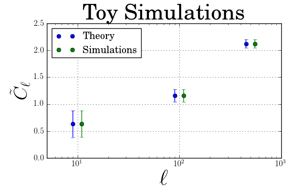
Figure 1: The mean and error bars given by the square root of the variance of a set of $10^{5}$ simulations are compared against the expected results in Equations (1) and (13). The differences are indistinguishable in the plot, and numerically differ by less than 0.3%, the expected deviation from $10^{5}$ simulations. In using test data that precisely match the assumptions used in deriving the mean and variance, these toy simulations verify that Equations (1) and (13) were derived correctly.

Secondly, in order to validate the analytical approximation to the full probability distribution, we bin the results of the above simulations and compare them against the integral of the probability distribution across the bin (Figure 2). In each case, the analytical approximation to the full probability distribution matches the simulations very well. The correspondence is not expected to be perfect. However, the analytical approximation is clearly superior to the Gaussian approximation at low to medium $\ell$, with the two becoming nearly indistinguishable at $\ell$ values of around a few hundred.

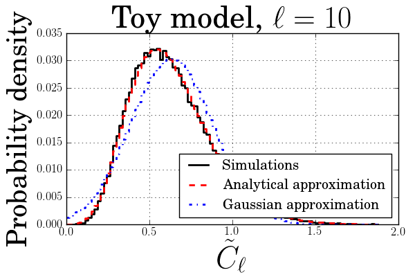
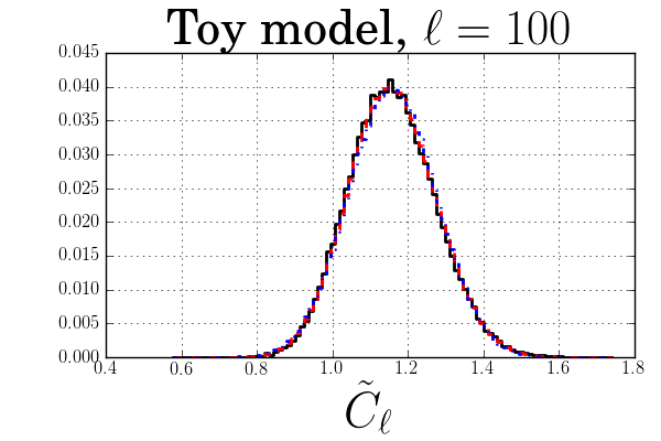
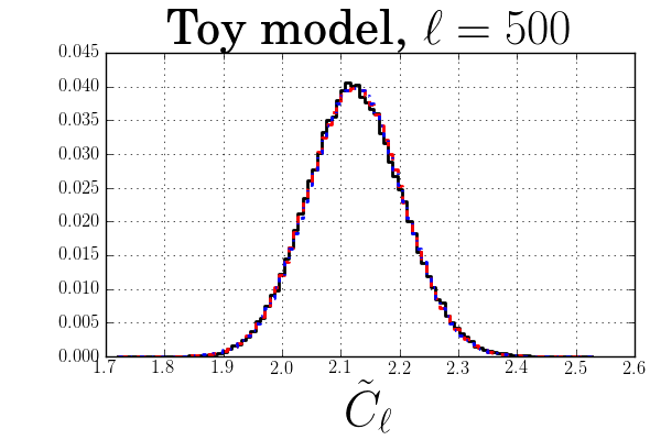
Figure 2: This test of the approximations to the probability distribution of $\tilde{C}_{\ell}$ shows that the analytical approximation, which models the probability as a sum of a chi-square distributed random variable and a Gaussian-distributed random variable, as well as a Gaussian approximation for comparison. While not perfect, the analytical approximation is better than the Gaussian at replicating the simulations. At high $\ell$, the Gaussian approximation and the analytical approximation become nearly indistinguishable in these plots.

3.2 Analysis of realistic simulations

In order to verify our likelihood function in a more realistic situation, we use a single realization of the foregrounds at all nine Planck frequency channels using the Planck Sky Model (described in Section 3.2.1). To the simulated foregrounds, we add a single realization of the noise. This realization is computed as uncorrelated, non-uniform noise, utilizing the same hit maps and per-sample variances as in Leach et al. (2008). To the simulated sky and noise we add a simulated lensed CMB using the LensPix software package (Lewis, 2005). A lensed CMB realization is used for the reason that the lensing breaks the assumption of complete independence of the $a_{\ell m}$ values, and is known to be a real feature in the observed CMB. Taking this non-ideality into account is thus important to help ensure that our method will be applicable to real data.

3.2.1 Planck Sky Model

Sky maps used in the present work are based on simulations obtained with the pre-launch Planck Sky Model software, a code designed to generate realistic full-sky maps of sky emission at millimetre wavelengths. A complete description of the PSM code is given in Delabrouille et al. (2012). We summarize here the main aspects of the particular simulation we use. To make a realization of the foregrounds, the PSM generates maps of different diffuse and compact source components, which are then coadded. For most of them, realizations are based on observed data sets, complemented by theoretical modelling where and when observations are missing. The map for each component is then computed at a set of observation frequencies on the basis of a modelled emission law for the component. In addition to CMB anisotropies, the components of sky emission implemented in the PSM include point sources (galactic and extragalactic), Sunyaev-Zel’dovich effects (thermal and kinetic), diffuse galactic emission, and fluctuations of the far infrared background emission from high redshift galaxies.

In the present simulations, diffuse emission from the galactic interstellar medium (ISM) is modelled as the sum of four main components: thermal emission of small dust particles heated by radiation from nearby stars; synchrotron emission, due to relativistic electrons spiralling in the galactic magnetic field; Free-free emission from warm regions of ionised interstellar gas; and the emission of small rotating dust grains.

The thermal dust emission is modelled on the basis of model 7 of Finkbeiner, Davis & Schlegel (1999). The total emission is represented as the sum of two modified blackbodies of the form:

$$I_{\nu}=\sum_{i=1}^{2}N_{i}\epsilon_{i}\nu^{\beta_{i}}B_{\nu}(T_{i})$$ (23)

where $B_{\nu}(T_{i})$ is the Planck function at temperature $T_{i}$, $N_{i}$ is the column density of species $i$, and $\epsilon_{i}\nu^{\beta_{i}}$ accounts for the normalization and frequency dependence of the emissivity.

Low frequency diffuse foregrounds (synchrotron, free-free ad spinning dust) are based on the analysis of WMAP observations performed by Miville-Deschênes et al. (2008). The synchrotron emission is obtained by scaling with a pixel-dependent emission law the template emission map observed at 408 MHz by Haslam et al. (1982). In the radio-mm frequency range, for an electron density following a power law of index $p$, ($ne(E)\propto E−p$), the synchrotron frequency dependence is also modelled as a power law:

$$I_{sync}(\nu)\propto\nu^{\beta_{s}+2}$$ (24)

where the spectral index is equal to $\beta_{s}=-(p+3)/2$. The synchrotron spectral index depends on cosmic ray properties. It varies with the direction on the sky, and possibly, with the frequency of observation (see, e.g., Strong, Moskalenko & Ptuskin (2007), for a review of propagation and interaction processes of cosmic rays in the Galaxy). The template synchrotron map obtained from Haslam et al., corrected for an offset monopole of $8.33K$ (Rayleigh-Jeans), is extrapolated in frequency on the basis of the spectral index map obtained from WMAP data.

Free-free is modelled on the basis of a template free-free map at 23 GHz, and a single universal emission law as given by Dickinson, Davies & Davis (2003).

In the PSM, the spinning dust emission is represented on the basis of a single template, together with a unique emission law which can be parametrised following the model of Draine & Lazarian (1998). The spinnning dust template is obtained by removing every other components contributing to the WMAP 23GHz data (free-free, synchrotron and thermal dust).

As the resolution of our simulation ($5$ arcmin) is better than that of the templates used to construct the model, small-scale fluctuations are added to Galactic emission simulations. The method used is described in Miville-Deschênes et al. (2007). A Gaussian random field $G_{ss}$ having a power spectrum defined as:

$$C_{l}=l^{\gamma}\left[e^{-l^{2}\sigma^{2}_{\mathrm{sim}}}-e^{l^{2}\sigma^{2}_{\mathrm{tem}}}\right]$$ (25)

is generated. Here $\sigma_{\mathrm{sim}}$ and $\sigma_{\mathrm{tem}}$ are the resolutions (in radian) of the simulation ($5^{\prime}$ here) and of the template to which small-scale fluctuations are added. The zero mean Gaussian field $G_{ss}$ is then normalized and multiplied by the template map exponentiated to a power $\beta$ in order to generate the proper amount of small-scale fluctuations as a function of local intensity. The resulting template map with small scale fluctuation added is then:

$$I^{\prime}_{\mathrm{tem}}=I_{\mathrm{tem}}+\alpha G_{ss}I^{\beta}_{\mathrm{tem}}$$ (26)

where $\alpha$ and $\beta$ are estimated for each template in order to make sure that the power spectrum of the small-scale structure added is in the continuity of the large scale part of the template.

The Sunyaev-Zel’dovich effect is modelled as the sum of two effects: thermal SZ effect which corresponds to the interaction of the CMB with a hot, thermalised electron gas, and the kinetic SZ effect which corresponds to CMB interaction with electrons having a net ensemble peculiar velocity along the line of sight. For thermal SZ, in the approximation of non-relativistic electrons, the change in sky brightness is:

$$\delta I_{\nu}=yf(\nu)B_{\nu}(T_{\mathrm{CMB}})$$ (27)

where $B_{ν}(T_{\mathrm{CMB}})$ is the CMB blackbody spectrum, $f(\nu)$ is a universal function of frequency that does not depend on the physical parameters of the electron population and $y$, the Compton parameter, is proportional to the integral along the line of sight of the electronic density $ne$ multiplied by the temperature of the electron gas:

$$\delta y=\int\frac{kT_{e}}{m_{e}c^{2}}n_{e}\sigma_{T}dl$$ (28)

where $T_{e}$ is the temperature of the electron gas, characterized by a Fermi distribution. The kinetic effect, due to the interaction of CMB photons with moving electrons, results in a shift of the photon distribution seen by an observer on Earth:

$$\delta I_{\nu}=-\beta_{r}\tau\left[\frac{\partial B_{\nu}(T)}{\partial T}\right]_{T=T_{\mathrm{CMB}}}$$ (29)

where $\beta_{r}$ is the dimensionless cluster velocity along the line of sight. The SZ simulation used in the present work is based on two different parts: hydro+N-body simulations of the distribution of baryons for redshifts $z<0.025$ obtained from Dolag et al. (2005), and pure N-body simulations of dark matter structures in a Hubble volume, using template from a smaller simulation by Schäfer et al. (2006).

Other compact sources are implemented as the sum of three populations: radio sources, infrared sources, and galactic ultra-compact HII regions.

Radio sources are simulated on the basis of both real radiosources observed around 1 and/or 5 GHz and on simulated sources generated at random to homogeneize the coverage where the sky surveys are shallow or incomplete. Sources fluxes are extrapolated to all frequencies required by the simulation using power law approximations of the spectra of the sources, of the form $S_{\nu}\propto\nu^{-\alpha}$ with different spectral indices in different frequency domains. Radio sources are divided in two populations, steep and flat, with typical spectral indexes distributed according to a Gaussian law with $\langle\alpha_{\mathrm{steep}}\rangle=1.18$ and $\langle\alpha_{\mathrm{flat}}\rangle=0.16$ respectively, and a variance of $\sigma_{\mathrm{steep,flat}}=0.3$.

IR sources are simulated on the basis of a compilation of sources observed by IRAS. Fluxes are extrapolated to useful frequencies using modified blackbody spectra $\nu^{b}B(\nu,T)$, $B(\nu,T)$ being the blackbody function. Again, randomly distributed sources are added until the mean surface density as a function of flux matches everywhere the mean of well covered regions.

The $864$ sources identified as ultra-compact Hii regions are treated separately from the above two populations. Their measured fluxes in the IRAS catalogues at $100$ and $60\,\mu m$, together with counterparts in the radio domain, are fitted with the sum of a modified blackbody and a free-free spectrum.

Finally, the PSM simulations include a background of unresolved high redshift faint sources (dusty and star forming galaxies), which is used to model anisotropies of the cosmic infrared background.

When all these components have been computed for all nine Planck frequencies, all observed component maps are then coadded to have a full-sky foreground map which is then added to our CMB and instrument noise simulations.

3.2.2 Masking

One of the difficulties with analyzing experimental data is that it is not possible to use the entire sky for the analysis, because experimental data may not cover the full sky in every channel, and because the brightest parts of the sky need to be masked to produce reliable results. Our method, if it is to be applicable to experimental data, needs to take this into account. This lack of full sky coverage breaks the assumption of independence of the $a_{\ell m}$ values. Therefore, we take the strategy of cutting as little of the sky as possible and hope that the assumption of independence is broken little enough that the analysis remains robust.

To this end, the masking strategy we use is to take 1.2% of the brightest pixels in each frequency map to make a mask at each frequency, then combine these masks to ensure any pixel masked in any frequency is masked. Point sources are not treated separately, though many of the brighter sources are masked through this method. In total, this cuts about 1.6% of the sky. Then, to prevent aliasing, we apodize the mask with a 33’ width apodization filter (33’ is the resolution of the 30 GHz channel). The apodization filter we use sets the value of any unmasked pixel equal to $e^{-\delta\theta^{2}/2\sigma^{2}}$ where $\delta\theta$ is the angular distance to the nearest masked pixel. This apodization filter ensures that all masked pixels remain completely masked, and both masked point sources and larger masked regions have similar apodization applied. For computational speed, any unmasked pixel that would have a value greater than 0.99 in the filter is left untouched. After applying the apodization, about 3.3% of the sky is removed in total. The sky fraction, $f_{\mathrm{sky}}=0.967$, is estimated using the average of the squares of the mask pixels, because the $a_{\ell m}$ values are squared when summing the power spectrum.

The particular masking level is chosen to ensure that the mask is as small as possible, to prevent correlations, while still not producing obviously wrong values for the low-$\ell$ power spectrum, as smaller masks tend to produce aliasing of the foreground signal into the low multipoles, resulting in one or more low-$\ell$ values being a couple of orders of magnitude larger than expected. Additionally, even slightly larger initial masks result in removing many more point sources which, after apodization, results in much larger sky fraction being removed (e.g. 7.1% removed in total with an initial mask size set to 1.5%).

Even when retaining a large fraction of sky, we risk biasing the estimated power spectrum by a few percent if we do not take the fractional coverage of sky into account. In order to make progress here, we write down the effect of the mask in harmonic space as follows:

$$\langle C_{\ell}^{\mathrm{masked}}\rangle={1\over 2\ell+1}\sum_{m=-\ell}^{\ell}\left(a_{\ell m}\odot w_{\ell m}\right)\left(a_{\ell m}\odot w_{\ell m}\right)^{*}.$$ (30)

Here the operator $\odot$ represents a convolution, which can be performed by converting the spherical harmonic transform of the mask $w_{\ell m}$ and the spherical harmonic transform of the CMB $a_{\ell m}$ back to pixel space and then multiplying the two together pixel by pixel. In practice, this process will mix the signals betwen different $m$ and $\ell$ values together. However, if we ignore the correlations induced by this process and assume statistical isotropy of the CMB, then we can represent the effect of the mask as a simple rescaling of the power spectrum:

$$\langle C_{\ell}^{\mathrm{masked}}\rangle={1\over N_{p}}\sum_{i=0}^{N_{p}-1}w_{i}^{2}{1\over 2\ell+1}\sum_{m=-\ell}^{\ell}a_{\ell m}a_{\ell m}^{*}.$$ (31)

Here $w_{i}$ represents the value of the mask at pixel $i$, with $w_{i}=1$ for pixels that are fully unmasked, $w_{i}=0$ for pixels fully masked, and values in between for pixels within the apodized region at the borders of the mask. We can thus represent this sum over the pixels in the mask as a single parameter:

$$f_{\mathrm{sky}}={1\over N_{p}}\sum_{i=0}^{N_{p}-1}w_{i}^{2}.$$ (32)

With this definition, we can write our final estimate of the probability distribution of $\tilde{C}_{\ell}$ as follows:

$$\langle\tilde{C}_{\ell}\rangle f_{\mathrm{sky}}=\left(1+{1-n_{c}\over n_{\mathrm{eff}}}\right)\langle C_{\ell}\rangle+{1\over\mathbf{e}^{\dagger}\hat{\mathbf{N}}_{\ell}^{-1}\mathbf{e}},$$ (33)

$$\langle\delta\tilde{C}_{\ell}^{2}\rangle f_{\mathrm{sky}}^{2}={2\langle C_{\ell}\rangle\over n_{\mathrm{eff}}}\left(\left(1+{1-n_{c}\over n_{\mathrm{eff}}}\right)\langle C_{\ell}\rangle+{2\over\mathbf{e}^{\dagger}\hat{\mathbf{N}}_{\ell}^{-1}\mathbf{e}}\right),$$ (34)

where $n_{\mathrm{eff}}=(2\ell+1)f_{\mathrm{sky}}$. The motivation for this change is that the primary effect of the mask is to apply a weight function to the $a_{\ell m}$ values so that instead of sums over $2\ell+1$ independent random variables, we have sums over $(2\ell+1)f_{\mathrm{sky}}$ independent random variables.

While the induced correlations between the $\tilde{C}_{\ell}$ values are not taken into account, it is our hope that keeping the masked region as small as possible minimizes the impact of this choice. In the following subsection we go over the tests we have used to ensure that at this level, the likelihood function is good enough to accurately capture the power spectrum and its uncertainties.

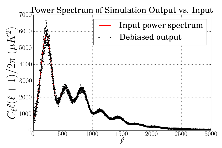
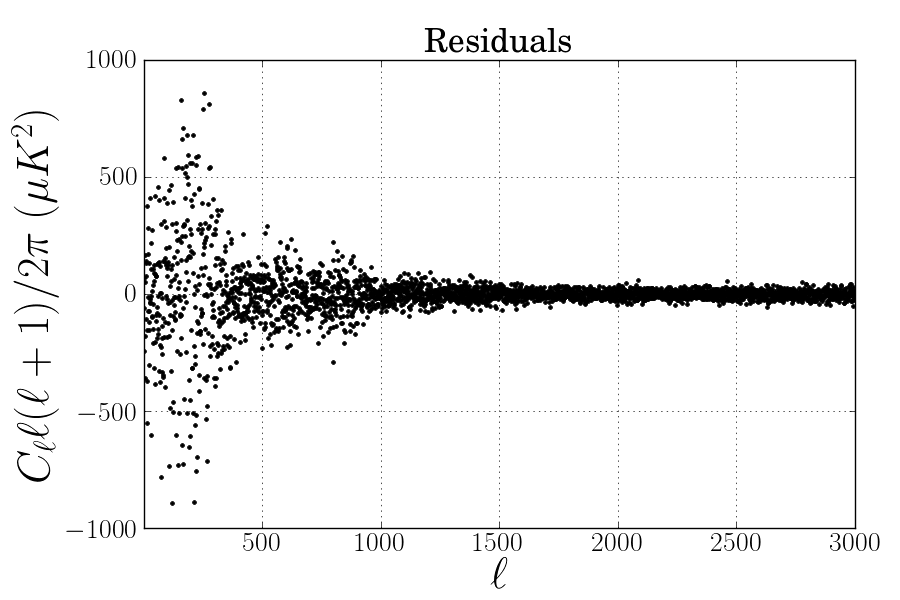
Figure 3: These figures compare the power spectra of the simulation input and of the component-separated results. Note that the debiasing which was performed assumed perfect knowledge of the foreground plus noise signal as well as input CMB, which significantly reduces the scatter, particularly at high $\ell$, compared to what would be available in an actual experiment. However, these plots are useful to visually demonstrate the validity of Equation (33) when applied to a realistic simulation. When used in an actual experiment, this equation would require factoring in the uncertainties in the foreground plus noise signal in some other manner. The primary conclusion here is that the mask, which removes 3.7% of the sky, does not impact the results in a manner which is clearly visible at the power spectrum level.

3.2.3 The Kolmogorov-Smirnov Test

In order to determine whether or not our approximation to the likelihood function is accurate, we make use of a Kolmogorov-Smirnov test, using the different $\ell$ values as different samples in the test. The K-S test compares the empirical cumulative probability distribution of a sample distribution with the theoretical cumulative probability distribution, and provides a statistic which can be used to evaluate whether or not the two distributions are the same.

The Kolmogorov-Smirnov statistic is the area that lies between the cumulative probability distributions of a test distribution and an empirical distribution. If the empirical distribution and the test distribution have the same shape, then this K-S statistic converges to zero. In fact, the convergence to zero occurs at a very specific rate depending upon the number of samples, if the two probability distributions are the same.

Correlations that are not accounted for in the test distribution will tend to reduce the rate at which the K-S statistic will converge to zero. To take a simple example, consider a situation where the test distribution assumes the samples are perfectly uncorrelated, while the input data sets every other value equal to the previous. With each value in the input data appearing twice, the K-S statistic will converge half as quickly, leading to a larger than expected K-S statistic.

Alternatively, if the input data have unmodeled anti-correlations, the reverse occurs and the K-S statistic converges more rapidly to zero than expected. A toy example here is to consider the situation where the test and empirical distributions both produce numbers between zero and one, but the empirical distribution sets every other number equal to one minus the previous. In this case, the K-S statistic will have encountered all of the independent numbers while iterating over only half of the range, which in practice speeds its convergence.

Thus by combining a $\chi^{2}$ test with the K-S statistic, we can obtain an estimate of both the shape of the distribution, which the $\chi^{2}$ test is sensitive to, and the correlations.

However, we cannot apply the K-S statistic directly with only one realization because the probability distribution of $\tilde{C}_{\ell}$ depends upon $\ell$. We can, however, perform a transformation on the random variable $\tilde{C}_{\ell}$ into some target probability distribution which is easily-estimated. A unit-variance Gaussian distribution is ideal here. Such transformation between different probability distributions is, for instance, routine in the generation of pseudorandom numbers. This is done by equating the cumulative probability distributions:

$${1\over\sqrt{2\pi}}\int_{-\infty}^{\chi_{\ell}}e^{x^{2}\over 2}dx=\int_{-\infty}^{\tilde{C}_{\ell}}P(\tilde{C}_{\ell}^{\prime})d\tilde{C}_{\ell}^{\prime}.$$ (35)

Note that for pseudorandom number generation, the source distribution is usually the uniform distribution on the interval $[0,1)$, for which the cumulative distribution is simply the random number itself. This sometimes masks the fact that what is being done is the equating of two cumulative distributions, making it appear as if one cumulative distribution is being equated to a random number. Our situation is not quite that simple.

Since the left hand side is the cumulative distribution of a unit-variance Gaussian distribution in one variable, we know the $\chi^{2}_{\ell}$ will follow a $\chi^{2}$ distribution with one degree of freedom. We convert to a Gaussian distribution first and then to a $\chi^{2}$ distribution because it is much simpler to invert the cumulative Gaussian distribution. The astute reader may note that the left hand side of the equation is simply related to the error function, and that we can compute $\chi^{2}_{\ell}$ using the inverse of the error function as follows:

$$\chi^{2}_{\ell}=2\left(\mathrm{erf}^{-1}\left(2\int_{-\infty}^{\tilde{C}_{\ell}}P(\tilde{C}_{\ell}^{\prime})d\tilde{C}_{\ell}^{\prime}-1\right)\right)^{2}.$$ (36)

If our approximation to the full probability distribution of $\tilde{C}_{\ell}$ is sufficiently accurate, then the $\chi^{2}_{\ell}$ for each $\ell$ follows a $\chi^{2}$ distribution with one degree of freedom. That is,

$$P(\chi^{2}_{\ell})={e^{-{\chi_{\ell}}^{2}\over 2}\over\sqrt{2\pi\chi_{\ell}^{2}}}.$$ (37)

For the inverse of the error function, we make use of an approximation with elementary functions produced by Sergei Winitzki, using methodology described in Winitzki (2003),

$$\mathrm{erf}^{-1}(x) \approx \mathrm{sgn}(x)\sqrt{\sqrt{\left(f(x)\right)^{2}-{\ln(1-x^{2})\over a}}-f(x)},$$ (38)

$$f(x) \equiv {2\over\pi a}+{\ln(1-x^{2})\over 2},$$ (39)

using the value of $a=0.147$ to keep the relative error at around the $10^{-4}$ level for all values of the argument of the inverse error function.

Note that while there are more computationally efficient methods to convert from some given probability distribution to a unit-variance Gaussian, they typically involve tricks such as combining two random numbers in non-trivial ways, or throwing away some random numbers. Neither of which would be an ideal solution here, as we only have a limited number of $\tilde{C}_{\ell}$ numbers to transform, and mixing multiple $\tilde{C}_{\ell}$ values would make the outcome for correlated or anti-correlated $\tilde{C}_{\ell}$ values difficult to predict. By using this direct transformation, the transformation reduces to what accounts to mostly a rescaling of the distribution of $\tilde{C}_{\ell}$ (as $\chi$ is monotonically increasing along with $\tilde{C}_{\ell}$). By just rescaling the distribution, we are likely to retain any correlations that exist, especially at higher $\ell$ where the rescaling is nearly uniform as $P(\tilde{C}_{\ell})$ approaches a Gaussian distribution.

Finally, in order to determine whether or not our computed value of the K-S statistic is reasonable, we compare this K-S statistic to a set of $10^{4}$ realizations of 2999 $\chi^{2}$-distributed independent random variables, quantifying the result using the fraction which provide a K-S statistic greater than the K-S statistic of our simulation result.

The results of these tests are that at the level of a single realization of the sky and over an $\ell$ range from $2-3000$, both the K-S statistic and the $\chi^{2}$ statistic lie within the 68% confidence limits. These results are shown in table 1.

$\chi^{2}$ test
	$\chi^{2}$	expected $\chi^{2}$
Analytical	2952	2999 $\pm$ 77.4
Gaussian	2956	2999 $\pm$ 77.4
K-S test
	K-S statistic (Da)	P(D $>$ Da)
Analytical	0.0138	0.60
Gaussian	0.0133	0.65

Table 1: The results of these statistical tests show that the probability distributions of the resultant $\tilde{C}_{\ell}$ values are in good accordance with the expected distributions to within the sample variance given by the $\ell$ range used. The K-S statistic found is within the one-sigma significance for both the Analytical and Gaussian estimates, indicating no significant unaccounted for net correlations or anti-correlations in the data. The expected error on the $\chi^{2}$ test comes from the variance of the $\chi^{2}$ distribution, which is twice the number of degrees of freedom. The probability P(D $>$ D_a) is the probability of obtaining a higher K-S statistic, as estimated by $10^{4}$ simulations of sets of 2999 $\chi^{2}$- distributed random variables. Values close to $0.5$ are expected.

4 Discussion

In this paper, we have presented a new likelihood function which can be used to estimate the likelihood of the CMB power spectrum given the data and a foreground model. Of particular interest is that with the simulations used in this paper, Planck data shows very little dependence on the foreground model until $\ell>2000$ or so, as shown in Figure 4. If true, this would be an indication that Planck has adequate frequency coverage for the level of diffuse foregrounds in temperature data.

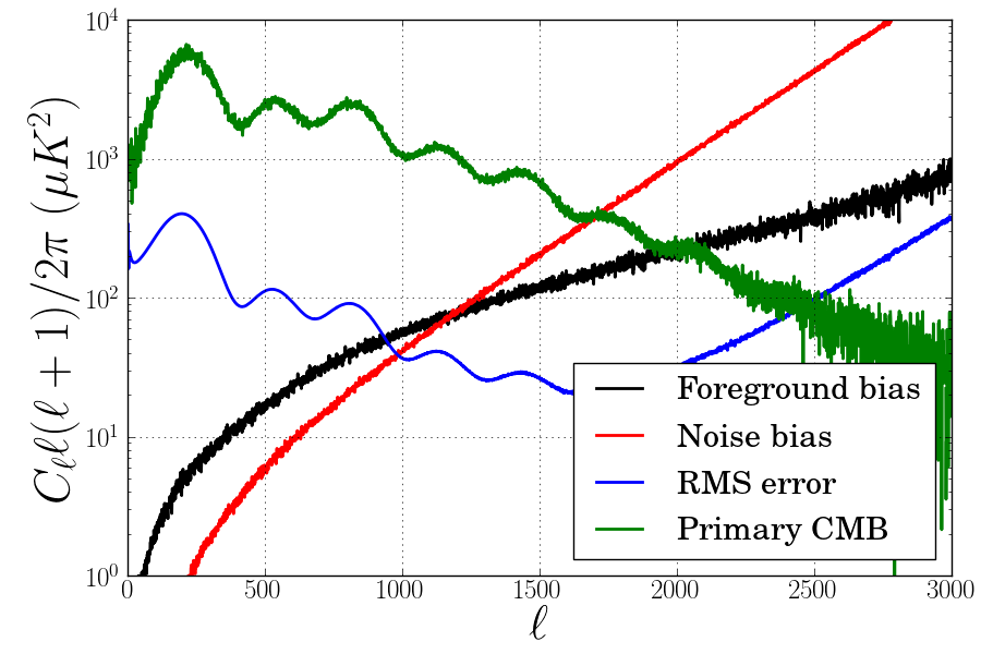
Figure 4: Comparison of the foreground and noise bias components against the debiased CMB power spectrum and an estimate of the RMS error. This estimate of the RMS error is based upon Equation (14), which adds a very rough estimate of the error due to the uncertainties in the foregrounds plus noise, assuming the foregrounds plus noise have a known power spectrum and are Gaussian-distributed. Because the foregrounds are negligible at low $\ell$ compared to cosmic variance, an accurate diffuse foreground model is probably not necessary. With the foregrounds becoming significant compared to the overall uncertainty at around $\ell>900$, an accurate compact source model is required, as the level of the foreground residuals becomes larger than the total expected error in the power spectrum. This supports the use of PSM-like simulations for diffuse foregrounds, with the uncertainties ignored, combined with a physical model for the compact foregrounds whose parameters are estimated along with the cosmological parameters.

For $\ell>1000$ or so, however, it is notable that in order to match the simulations, we need not only a model of instrument noise, but also the foreground model. This is an indication that compact sources remain a significant factor in the data. From these tests, it would be perfectly reasonable to make use of a fixed Galactic foreground model combined with a power spectrum-based compact source model, such as that used in Millea et al. (2011). This is very much an ideal situation because the parameters that impact the power spectra of compact sources can be very well-estimated at the power spectrum level.

The most accurate way of including the instrument noise contribution would probably be to pre-compute the spherical harmonic transforms of a set of simulations of the full instrument noise. While the number of noise simulations is likely to be much smaller than the number of Monte Carlo simulations in the full parameter estimation analysis, a thousand or so noise simulations should be sufficient to effectively marginalize over instrument noise. This method would have the advantage of incorporating the full instrument noise covariance, if sufficiently-detailed noise simulations are used, albeit in an approximate manner. Care would need to be taken to ensure that the use of the simulations within the parameter-estimation MCMC chain do not require significant computing resources. One might also imagine simpler approximations such as that used in Equation (14).

Therefore we would recommend making use of the probability function $P(\tilde{C}_{\ell}|C_{\ell},N_{\ell})$, where $N_{\ell}=1/e^{\dagger}\hat{\mathbf{N}}_{\ell}^{-1}e$, with $\hat{\mathbf{N}}_{\ell}$ being the estimated covariance of the instrument noise plus foreground model which depends upon any foreground parameters which are to be marginalized over.

Once the details of the foreground plus noise models are determined, the work in this paper demonstrates that provided the mask removes very little of the sky, the likelihood function we supply provides a reasonably accurate estimate of the true likelihood of the CMB in the presence of foregrounds. However, it does have difficulties at low multipoles, as can be seen through a cursory examination of Equation (1). In particular the second term, $(1-n_{c})/(2\ell+1)\langle C_{\ell}\rangle$, represents the statistical component of the ILC bias. Note that the denominator is the number of $a_{\ell m}$ terms that go into the average for this power spectrum component.

Perhaps a useful comparison of how significant this bias term is would be to compare it against the fact that other power spectrum estimation codes use a much smaller fraction of the sky in their analysis with a similar impact on the error that results. If we are to compare against a method which uses 80% sky coverage, for instance, a back-of-the-envelope calculation would suggest that we want our statistical bias term to be no more than about 15% or so of the power spectrum, indicating we should have a better estimate of the errors for roughly $\ell>50$ as compared with such a hypothetical method. While some may be nervous about trusting our estimate of the errors in the intermediate $\ell$ range of around $50<\ell<400$ or so, our simulations indicate that the residual foreground contamination in this range is more than an order of magnitude below the estimated total error in the power spectrum.

Additionally, it might be worthwhile to consider binning the power spectrum in order to reduce the magnitude of the statistical bias term. However, binning the power spectrum does destroy some information about the CMB power, and it may potentially increase the foreground bias term, so we do not consider that here. One additional possibility is a hybrid method: estimate the ILC weights on bins in $\ell$, but extract the power spectrum separately at each $\ell$. This has the benefit of reducing the statistical bias term while retaining full resolution on the CMB power. However, it has the drawback that it likely increases the foreground bias term, while at the same time inducing correlations between each $\tilde{C}_{\ell}$ within a bin.

While it is in principle possible to estimate the correlation within each bin, at very low-$\ell$ the likelihood function is non-Gaussian, and it is an extremely non-trivial problem to consider both the correlations and the non-Gaussianity of the low-$\ell$ power spectrum at the same time. There is, however, an intermediate range in $\ell$, around $\ell=100$ to $\ell=400$ or so, where the statistical bias term is non-negligible but the likelihood function highly Gaussian where this approach may be tractable. But due to the work involved for what is likely to be a very small improvement in the CMB uncertainty (of the order of a few percent in the variance in $\tilde{C}_{\ell}$), we do not consider this approach here.

Another potential question is why we do not suggest simply making use of a model of the foregrounds given by the data minus the estimated CMB. As we show in Appendix B, using this as the foreground model gives identically zero for the estimate of the foreground contamination. In fact, this calculation places into doubt any sort of “boot strapping”-type estimation of the foreground subtraction errors: it is absolutely required to have some physical model of the foregrounds in order to estimate the foreground subtraction errors.

This paper also begs the question that if we require a foreground model such as that used in Millea et al. (2011), why go through the work of implementing the ILC at all? Why not simply make use of the parametric model of the foregrounds? Our argument here is that because the ILC method significantly reduces the foregrounds prior to the likelihood analysis, this method will be less sensitive to the precise details of the foreground model used, permitting a greater level of uncertainty in the foreground model before cosmological parameters are impacted. This is particularly the case at high $\ell$ when we are no longer limited by cosmic variance.

Appendix A Variance Calculation

In order to compute the variance of the estimated power spectrum, we start with Equation (13), the square of which is:

$$\delta\tilde{C}_{\ell}^{2} =$$ (40)

$$\delta C_{\ell}^{2}+\left({1-n_{c}\over 2\ell+1}\langle C_{\ell}\rangle\right)^{2}+\left(\mathbf{f}^{\dagger}_{\ell}\hat{\mathbf{N}}_{\ell}^{-1}\mathbf{f}_{\ell}\right)^{2}+\left({\mathbf{e}^{\dagger}\hat{\mathbf{N}}_{\ell}^{-1}\mathbf{f}_{\ell}+\mathbf{f}^{\dagger}_{\ell}\hat{\mathbf{N}}_{\ell}^{-1}\mathbf{e}\over\mathbf{e}^{\dagger}\hat{\mathbf{N}}_{\ell}^{-1}\mathbf{e}}\right)^{2}+\left({\mathbf{e}^{\dagger}\hat{\mathbf{N}}_{\ell}^{-1}\mathbf{f}_{\ell}\mathbf{f}^{\dagger}_{\ell}\hat{\mathbf{N}}_{\ell}^{-1}\mathbf{e}\over\mathbf{e}^{\dagger}\hat{\mathbf{N}}_{\ell}^{-1}\mathbf{e}}\right)^{2}$$

$$+2\delta C_{\ell}\left({1-n_{c}\over 2\ell+1}\langle C_{\ell}\rangle-\mathbf{f}^{\dagger}_{\ell}\hat{\mathbf{N}}_{\ell}^{-1}\mathbf{f}_{\ell}+{\mathbf{e}^{\dagger}\hat{\mathbf{N}}_{\ell}^{-1}\mathbf{f}_{\ell}+\mathbf{f}^{\dagger}_{\ell}\hat{\mathbf{N}}_{\ell}^{-1}\mathbf{e}+\mathbf{e}^{\dagger}\hat{\mathbf{N}}_{\ell}^{-1}\mathbf{f}_{\ell}\mathbf{f}^{\dagger}_{\ell}\hat{\mathbf{N}}_{\ell}^{-1}\mathbf{e}\over\mathbf{e}^{\dagger}\hat{\mathbf{N}}_{\ell}^{-1}\mathbf{e}}\right)$$

$$+2\left({1-n_{c}\over 2\ell+1}\right)\langle C_{\ell}\rangle\left(-\mathbf{f}^{\dagger}_{\ell}\hat{\mathbf{N}}_{\ell}^{-1}\mathbf{f}_{\ell}+{\mathbf{e}^{\dagger}\hat{\mathbf{N}}_{\ell}^{-1}\mathbf{f}_{\ell}+\mathbf{f}^{\dagger}_{\ell}\hat{\mathbf{N}}_{\ell}^{-1}\mathbf{e}+\mathbf{e}^{\dagger}\hat{\mathbf{N}}_{\ell}^{-1}\mathbf{f}_{\ell}\mathbf{f}^{\dagger}_{\ell}\hat{\mathbf{N}}_{\ell}^{-1}\mathbf{e}\over\mathbf{e}^{\dagger}\hat{\mathbf{N}}_{\ell}^{-1}\mathbf{e}}\right)$$

$$-2\mathbf{f}^{\dagger}_{\ell}\hat{\mathbf{N}}_{\ell}^{-1}\mathbf{f}_{\ell}\left({\mathbf{e}^{\dagger}\hat{\mathbf{N}}_{\ell}^{-1}\mathbf{f}_{\ell}+\mathbf{f}^{\dagger}_{\ell}\hat{\mathbf{N}}_{\ell}^{-1}\mathbf{e}+\mathbf{e}^{\dagger}\hat{\mathbf{N}}_{\ell}^{-1}\mathbf{f}_{\ell}\mathbf{f}^{\dagger}_{\ell}\hat{\mathbf{N}}_{\ell}^{-1}\mathbf{e}\over\mathbf{e}^{\dagger}\hat{\mathbf{N}}_{\ell}^{-1}\mathbf{e}}\right)$$

$$+2\left({\mathbf{e}^{\dagger}\hat{\mathbf{N}}_{\ell}^{-1}\mathbf{f}_{\ell}+\mathbf{f}^{\dagger}_{\ell}\hat{\mathbf{N}}_{\ell}^{-1}\mathbf{e}\over\mathbf{e}^{\dagger}\hat{\mathbf{N}}_{\ell}^{-1}\mathbf{e}}\right)\left({\mathbf{e}^{\dagger}\hat{\mathbf{N}}_{\ell}^{-1}\mathbf{f}_{\ell}\mathbf{f}^{\dagger}_{\ell}\hat{\mathbf{N}}_{\ell}^{-1}\mathbf{e}\over\mathbf{e}^{\dagger}\hat{\mathbf{N}}_{\ell}^{-1}\mathbf{e}}\right).$$

This equation seems quite daunting, however when we take the expectation value, many of the terms turn out to be zero. The first aspect which we exploit is that only even products of the $a_{\ell m}$ coefficients have non-zero expectation value. Note that $\mathbf{f}_{\ell}$ is linear in $a_{\ell m}$, while $C_{\ell}$ goes as the square of $a_{\ell m}$. Additionally, because $\hat{\mathbf{N}}_{\ell}$ is a real, symmetric matrix, $\mathbf{e}^{\dagger}\hat{\mathbf{N}}_{\ell}^{-1}\mathbf{f}_{\ell}=\mathbf{f}^{\dagger}_{\ell}\hat{\mathbf{N}}_{\ell}^{-1}\mathbf{e}$. Combining these two statements along with $\langle\delta C_{\ell}\rangle=0$ gives:

$$\langle\delta\tilde{C}_{\ell}^{2}\rangle =$$ (41)

$$\left\langle\delta C_{\ell}^{2}+\left({1-n_{c}\over 2\ell+1}\langle C_{\ell}\rangle\right)^{2}+\left(\mathbf{f}^{\dagger}_{\ell}\hat{\mathbf{N}}_{\ell}^{-1}\mathbf{f}_{\ell}\right)^{2}+\left({2\mathbf{e}^{\dagger}\hat{\mathbf{N}}_{\ell}^{-1}\mathbf{f}_{\ell}\over\mathbf{e}^{\dagger}\hat{\mathbf{N}}_{\ell}^{-1}\mathbf{e}}\right)^{2}+{\left(\mathbf{e}^{\dagger}\hat{\mathbf{N}}_{\ell}^{-1}\mathbf{f}_{\ell}\right)^{4}\over\left(\mathbf{e}^{\dagger}\hat{\mathbf{N}}_{\ell}^{-1}\mathbf{e}\right)^{2}}\right.$$

$$+2\delta C_{\ell}\left(-\mathbf{f}^{\dagger}_{\ell}\hat{\mathbf{N}}_{\ell}^{-1}\mathbf{f}_{\ell}+{\left(\mathbf{e}^{\dagger}\hat{\mathbf{N}}_{\ell}^{-1}\mathbf{f}_{\ell}\right)^{2}\over\mathbf{e}^{\dagger}\hat{\mathbf{N}}_{\ell}^{-1}\mathbf{e}}\right)+2\left({1-n_{c}\over 2\ell+1}\right)\langle C_{\ell}\rangle\left(-\mathbf{f}^{\dagger}_{\ell}\hat{\mathbf{N}}_{\ell}^{-1}\mathbf{f}_{\ell}+{\left(\mathbf{e}^{\dagger}\hat{\mathbf{N}}_{\ell}^{-1}\mathbf{f}_{\ell}\right)^{2}\over\mathbf{e}^{\dagger}\hat{\mathbf{N}}_{\ell}^{-1}\mathbf{e}}\right)$$

$$-2\left.\mathbf{f}^{\dagger}_{\ell}\hat{\mathbf{N}}_{\ell}^{-1}\mathbf{f}_{\ell}{\left(\mathbf{e}^{\dagger}\hat{\mathbf{N}}_{\ell}^{-1}\mathbf{f}_{\ell}\right)^{2}\over\mathbf{e}^{\dagger}\hat{\mathbf{N}}_{\ell}^{-1}\mathbf{e}}\right\rangle.$$

From here, we need to individually compute the expectation values of each component. This is done using the known expectation values of the $a_{\ell m}$ coefficients:

$$\langle a_{\ell m_{1}}a^{*}_{\ell m_{2}}\rangle = \langle C_{\ell}\rangle\delta_{m_{1}m_{2}},$$ (42)

$$\langle a_{\ell m_{1}}a^{*}_{\ell m_{2}}a_{\ell m_{3}}a^{*}_{\ell m_{4}}\rangle = \langle C_{\ell}\rangle^{2}\left(\delta_{m_{1}m_{2}}\delta_{m_{3}m_{4}}+\delta_{m_{1}m_{4}}\delta_{m_{2}m_{3}}+\delta_{m_{1}-m_{3}}\delta_{m_{2}-m_{4}}\right).$$ (43)

Here we describe in detail the calculation of one of the more complicated terms, and simply list the answers for the remaining terms. Perhaps the most complicated term is the final one, which requires taking the expectation value of the following:

$$\left\langle{\mathbf{f}^{\dagger}_{\ell}\hat{\mathbf{N}}_{\ell}^{-1}\mathbf{f}_{\ell}\left(\mathbf{e}^{\dagger}\hat{\mathbf{N}}_{\ell}^{-1}\mathbf{f}_{\ell}\right)^{2}\over\mathbf{e}^{\dagger}\hat{\mathbf{N}}_{\ell}^{-1}\mathbf{e}}\right\rangle=\left\langle{\mathbf{f}^{\dagger}_{\ell}\hat{\mathbf{N}}_{\ell}^{-1}\mathbf{f}_{\ell}\mathbf{f}^{\dagger}_{\ell}\hat{\mathbf{N}}_{\ell}^{-1}\mathbf{e}\mathbf{e}^{\dagger}\hat{\mathbf{N}}_{\ell}^{-1}\mathbf{f}_{\ell}\over\mathbf{e}^{\dagger}\hat{\mathbf{N}}_{\ell}^{-1}\mathbf{e}}\right\rangle.$$ (44)

We expand the square in this particular way in order to ensure that when expanded fully, the $a_{\ell m}$ coefficients would have the same order of complex conjugation as in Equation (43). The full expansion is done by using the definition of $\mathbf{f}_{\ell}$ in Equation (8). Note that the conjugate transpose of $\mathbf{f}_{\ell}$ is then defined as follows:

$$\mathbf{f}_{\ell}^{\dagger}\equiv\sum_{m=-\ell}^{\ell}a_{\ell m}\mathbf{f}_{\ell m}^{\dagger}.$$ (45)

With these definitions, Equation (44) becomes:

$$\left\langle{\mathbf{f}^{\dagger}_{\ell}\hat{\mathbf{N}}_{\ell}^{-1}\mathbf{f}_{\ell}\mathbf{f}^{\dagger}_{\ell}\hat{\mathbf{N}}_{\ell}^{-1}\mathbf{e}\mathbf{e}^{\dagger}\hat{\mathbf{N}}_{\ell}^{-1}\mathbf{f}_{\ell}\over\mathbf{e}^{\dagger}\hat{\mathbf{N}}_{\ell}^{-1}\mathbf{e}}\right\rangle =$$

$${1\over(2\ell+1)^{4}} \sum_{m_{1}=-\ell}^{\ell}\sum_{m_{2}=-\ell}^{\ell}\sum_{m_{3}=-\ell}^{\ell}\sum_{m_{4}=-\ell}^{\ell}\langle a_{\ell m_{1}}a^{*}_{\ell m_{2}}a_{\ell m_{3}}a^{*}_{\ell m_{4}}\rangle{\mathbf{f}_{\ell m_{1}}^{\dagger}\hat{\mathbf{N}}_{\ell}^{-1}\mathbf{f}_{\ell m_{2}}\mathbf{f}_{\ell m_{3}}^{\dagger}\hat{\mathbf{N}}_{\ell}^{-1}\mathbf{e}\mathbf{e}^{\dagger}\hat{\mathbf{N}}_{\ell}^{-1}\mathbf{f}_{\ell m_{4}}\over\mathbf{e}^{\dagger}\hat{\mathbf{N}}_{\ell}^{-1}\mathbf{e}}.$$ (46)

We can then make use of the definition of $\hat{\mathbf{N}}_{\ell}$, which is:

$$\hat{\mathbf{N}}_{\ell}\equiv{1\over 2\ell+1}\sum_{m=-\ell}^{\ell}\mathbf{f}_{\ell m}\mathbf{f}_{\ell m}^{\dagger},$$ (47)

as well as Equation (43) and the fact that $\mathbf{f}_{\ell m}^{*}=\mathbf{f}_{\ell-m}$ to give:

$$\left\langle{\mathbf{f}^{\dagger}_{\ell}\hat{\mathbf{N}}_{\ell}^{-1}\mathbf{f}_{\ell}\mathbf{f}^{\dagger}_{\ell}\hat{\mathbf{N}}_{\ell}^{-1}\mathbf{e}\mathbf{e}^{\dagger}\hat{\mathbf{N}}_{\ell}^{-1}\mathbf{f}_{\ell}\over\mathbf{e}^{\dagger}\hat{\mathbf{N}}_{\ell}^{-1}\mathbf{e}}\right\rangle={\langle C_{\ell}\rangle^{2}\over(2\ell+1)^{2}}\left({\mathbf{Tr[\hat{\mathbf{N}}_{\ell}^{-1}\hat{\mathbf{N}}_{\ell}]\mathbf{e}^{\dagger}\hat{\mathbf{N}}_{\ell}^{-1}\hat{\mathbf{N}}_{\ell}\hat{\mathbf{N}}_{\ell}^{-1}\mathbf{e}}\over\mathbf{e}^{\dagger}\hat{\mathbf{N}}_{\ell}^{-1}\mathbf{e}}+2{\mathbf{e}^{\dagger}\hat{\mathbf{N}}_{\ell}^{-1}\hat{\mathbf{N}}_{\ell}\hat{\mathbf{N}}_{\ell}^{-1}\hat{\mathbf{N}}_{\ell}\hat{\mathbf{N}}_{\ell}^{-1}\mathbf{e}\over\mathbf{e}^{\dagger}\hat{\mathbf{N}}_{\ell}^{-1}\mathbf{e}}\right).$$ (48)

Since the trace of the identity matrix is simply the number of channels, this expectation value simplifies to:

$$\left\langle{\mathbf{f}^{\dagger}_{\ell}\hat{\mathbf{N}}_{\ell}^{-1}\mathbf{f}_{\ell}\mathbf{f}^{\dagger}_{\ell}\hat{\mathbf{N}}_{\ell}^{-1}\mathbf{e}\mathbf{e}^{\dagger}\hat{\mathbf{N}}_{\ell}^{-1}\mathbf{f}_{\ell}\over\mathbf{e}^{\dagger}\hat{\mathbf{N}}_{\ell}^{-1}\mathbf{e}}\right\rangle={\langle C_{\ell}\rangle^{2}\over(2\ell+1)^{2}}\left(n_{c}+2\right).$$ (49)

The expectation values of the remaining terms in Equation (41) are:

$$\langle\delta C_{\ell}^{2}\rangle = {2\langle C_{\ell}\rangle^{2}\over 2\ell+1},$$ (50)

$$\left\langle\left(\mathbf{f}^{\dagger}_{\ell}\hat{\mathbf{N}}_{\ell}^{-1}\mathbf{f}_{\ell}\right)^{2}\right\rangle = \langle C_{\ell}\rangle^{2}{n_{c}^{2}+2n_{c}\over(2\ell+1)^{2}},$$ (51)

$$\left\langle{\mathbf{e}^{\dagger}\hat{\mathbf{N}}_{\ell}^{-1}\mathbf{f}_{\ell}\mathbf{f}^{\dagger}_{\ell}\hat{\mathbf{N}}_{\ell}^{-1}\mathbf{e}\over\left(\mathbf{e}^{\dagger}\hat{\mathbf{N}}_{\ell}^{-1}\mathbf{e}\right)^{2}}\right\rangle = {\langle C_{\ell}\rangle\over(2\ell+1)\mathbf{e}^{\dagger}\hat{\mathbf{N}}_{\ell}^{-1}\mathbf{e}},$$ (52)

$$\left\langle\left({\mathbf{e}^{\dagger}\hat{\mathbf{N}}_{\ell}^{-1}\mathbf{f}_{\ell}\mathbf{f}^{\dagger}_{\ell}\hat{\mathbf{N}}_{\ell}^{-1}\mathbf{e}\over\mathbf{e}^{\dagger}\hat{\mathbf{N}}_{\ell}^{-1}\mathbf{e}}\right)^{2}\right\rangle = {3\langle C_{\ell}\rangle^{2}\over(2\ell+1)^{2}},$$ (53)

$$\left\langle\delta C_{\ell}\mathbf{f}^{\dagger}_{\ell}\hat{\mathbf{N}}_{\ell}^{-1}\mathbf{f}_{\ell}\right\rangle = {2\langle C_{\ell}\rangle^{2}n_{c}\over(2\ell+1)^{2}},$$ (54)

$$\left\langle\delta C_{\ell}{\mathbf{e}^{\dagger}\hat{\mathbf{N}}_{\ell}^{-1}\mathbf{f}_{\ell}\mathbf{f}^{\dagger}_{\ell}\hat{\mathbf{N}}_{\ell}^{-1}\mathbf{e}\over\mathbf{e}^{\dagger}\hat{\mathbf{N}}_{\ell}^{-1}\mathbf{e}}\right\rangle = {2\langle C_{\ell}\rangle^{2}\over(2\ell+1)^{2}},$$ (55)

$$\left\langle\mathbf{f}^{\dagger}_{\ell}\hat{\mathbf{N}}_{\ell}^{-1}\mathbf{f}_{\ell}\right\rangle = {\langle C_{\ell}\rangle n_{c}\over 2\ell+1},$$ (56)

$$\left\langle{\mathbf{e}^{\dagger}\hat{\mathbf{N}}_{\ell}^{-1}\mathbf{f}_{\ell}\mathbf{f}^{\dagger}_{\ell}\hat{\mathbf{N}}_{\ell}^{-1}\mathbf{e}\over\mathbf{e}^{\dagger}\hat{\mathbf{N}}_{\ell}^{-1}\mathbf{e}}\right\rangle = {\langle C_{\ell}\rangle\over 2\ell+1}.$$ (57)

Substituting these expectation values into Equation (41) gives:

$$\langle\delta\tilde{C}_{\ell}^{2}\rangle= {\langle C_{\ell}\rangle\over 2\ell+1}\left(2\langle C_{\ell}\rangle+{(1-n_{c})^{2}\langle C_{\ell}\rangle\over 2\ell+1}+\langle C_{\ell}\rangle{n_{c}^{2}+2n_{c}\over 2\ell+1}+{4\over\mathbf{e}^{\dagger}\hat{\mathbf{N}}_{\ell}^{-1}\mathbf{e}}+{3\langle C_{\ell}\rangle\over 2\ell+1}-{4\langle C_{\ell}\rangle n_{c}\over 2\ell+1}+{4\langle C_{\ell}\rangle\over 2\ell+1}\right.$$ (58)

$$\left.-{1-n_{c}\over 2\ell+1}2\langle C_{\ell}\rangle(-n_{c}+1)-{2\langle C_{\ell}\rangle\over 2\ell+1}(n_{c}+2)\right),$$

which simplifies to:

$$\langle\delta\tilde{C}_{\ell}^{2}\rangle={2\langle C_{\ell}\rangle\over 2\ell+1}\left(\langle C_{\ell}\rangle+{1-n_{c}\over 2\ell+1}\langle C_{\ell}\rangle+{2\over\mathbf{e}^{\dagger}\hat{\mathbf{N}}_{\ell}^{-1}\mathbf{e}}\right).$$ (59)

Appendix B On the Need for a Physical Model

There are significant difficulties in developing an accurate physical model for the foreground signal. For diffuse Galactic foregrounds, variation along the line of sight of the foreground properties (such as the dust temperature) have the potential to significantly complicate the modeling of the foreground. For compact sources, the spectra of these sources may vary significantly depending upon the source, and may show some variation over the age of the universe as well, which would make the process of validating compact source spectra by using the nearby bright sources a questionable proposition. Therefore, an absolutely ideal situation would be one in which we are able to ignore the potential difficulties of finding an accurate model for foreground emission and are able to extract the primary CMB signal without worrying about the details of the foregrounds.

This may be one of the motivating factors for the use of so many blind component separation methods, such as the many variations of ILC and ICA that have been used. In fact, it is often impressive how well these component separation methods do at removing the foregrounds. However, as we argue is the case here for ILC in harmonic space, there is no way to estimate the actual errors in the removal without a physical model. To do this, we examine the case where instead of having a physical model for the covariance of the foregrounds $\hat{\mathbf{N}}_{\ell}$, we make use of an estimate of the foreground signal given by:

$$\tilde{\mathbf{f}}_{\ell m}=\mathbf{d}_{\ell m}-\tilde{a}_{\ell m}.$$ (60)

Here $\tilde{\mathbf{f}}_{\ell m}$ is the spherical harmonic transform of our estimate of the foreground signal at each observation frequency, $\mathbf{d}_{\ell m}$ is the spherical harmonic transform of the data at each frequency, and $\tilde{a}_{\ell m}$ is the spherical harmonic transform of our estimate of the CMB sky through harmonic-space ILC.

With these definitions, it is easy to show that the covariance matrix at each $\ell$ of our estimate of the foreground signal is given by:

$$\tilde{\mathbf{N}}_{\ell}=\hat{\mathbf{C}}_{\ell}-\mathbf{e}\mathbf{e}^{\dagger}\tilde{C}_{\ell}.$$ (61)

To understand how the use of this estimate of the foreground signal affects our results, we need to use this estimate for the term that encodes the effect of the foreground power spectrum in our bias and variance estimates, $1/e^{\dagger}\tilde{\mathbf{N}}_{\ell}^{-1}e$. To facilitate the calculation of this statement, we write $\tilde{\mathbf{N}}_{\ell}$ by expanding $\hat{\mathbf{C}}_{\ell}$ in terms of its CMB and foreground components as follows:

$$\tilde{\mathbf{N}}_{\ell}=\mathbf{e}\mathbf{e}^{\dagger}(C_{\ell}-\tilde{C}_{\ell})+\mathbf{e}\mathbf{f}_{\ell}^{\dagger}+\mathbf{f}_{\ell}\mathbf{e}^{\dagger}+\hat{\mathbf{N}}_{\ell}.$$ (62)

Because of the similarity of Equation (62) with (9), we can simply write down the result as a slight modification of Equation (10):

$${1\over e^{\dagger}\tilde{\mathbf{N}}_{\ell}^{-1}e} = C_{\ell}-\tilde{C}_{\ell}$$ (63)

$$+{1+\mathbf{e}^{\dagger}\hat{\mathbf{N}}_{\ell}^{-1}\mathbf{f}_{\ell}+\mathbf{f}^{\dagger}_{\ell}\hat{\mathbf{N}}_{\ell}^{-1}\mathbf{e}+\mathbf{e}^{\dagger}\hat{\mathbf{N}}_{\ell}^{-1}\mathbf{f}_{\ell}\mathbf{f}^{\dagger}_{\ell}\hat{\mathbf{N}}_{\ell}^{-1}\mathbf{e}\over\mathbf{e}^{\dagger}\hat{\mathbf{N}}_{\ell}^{-1}\mathbf{e}}$$

$$-\mathbf{f}^{\dagger}_{\ell}\hat{\mathbf{N}}_{\ell}^{-1}\mathbf{f}_{\ell}$$

$$= \tilde{C}_{\ell}-\tilde{C}_{\ell}=0.$$ (64)

Thus, by using this simplified estimate of the foreground signal, all information about the foreground contamination, both in the bias and variance, is destroyed. While we could, in principle, add something to $\tilde{C}_{\ell}$ to make it so that $1/e^{\dagger}\tilde{\mathbf{N}}^{+}e\neq 0$, the difference between $1/e^{\dagger}\tilde{\mathbf{N}}^{+}e$ and zero will just be a function of the arbitrary offset and not provide us with any new information about the foreground signal.

Furthermore, though our calculation is performed on a term which was derived assuming uncorrelated CMB samples, Delabrouille et al. (2009) argue that this sort of calculation can be used as an approximation to the true bias even with correlated samples, at least within the Needlet framework. Therefore, to first order, the effect of the foreground contamination is canceled in the case of correlated CMB samples. Higher-order terms arising from the correlations may cause some information about the bias to be recovered, but with most of the information destroyed by this method, it is unlikely to be useful. This has direct implications upon the bias calculated by the WMAP team in Hinshaw et al. (2007), as their estimation of the bias through simulations directly mirrors the methodology of the calculation performed in this Appendix. This indicates that the bias used in computing the ILC map published by the WMAP team likely misses most of the actual ILC bias, and may have higher-order contributions which are not understood and may, in certain cases, even have the wrong sign. Similarly, Kim, Naselsky & Christensen (2008) also makes use of an estimate of the foregrounds as being the data minus their ILC-estimated CMB, and therefore likely underestimates the bias as well.

This calculation seems to argue that in order to obtain an accurate estimate of the errors and biases in the ILC method, it is fundamentally required to have a physical, parametric model of the foregrounds. It is, in principle, possible to make use of simulated foregrounds. However as our likelihood function in Equation (22) demonstrates, the probability distribution of $\tilde{C}_{\ell}$ depends both upon the cosmological model and upon the foreground model, and it is very difficult to vary both in a simulation environment. There is the additional concern that some of the foregrounds, such as SZ clusters, would also depend upon the cosmological model in a detailed treatment.

References

- Amblard, Cooray & Kaplinghat (2007) Amblard A., Cooray A., Kaplinghat M., 2007, Phys. Rev. D, 75, 083508
- Basak & Delabrouille (2012) Basak S., Delabrouille J., 2012, MNRAS, 419, 1163
- Bennett et al. (2003) Bennett C. L. et al., 2003, astro-ph/0302207
- Delabrouille et al. (2009) Delabrouille J., Cardoso J.-F., Le Jeune M., Betoule M., Fay G., Guilloux F., 2009, A&A, 493, 835
- Delabrouille et al. (2012) Delabrouille J. et al., 2012, arXiv in prep
- Dick, Remazeilles & Delabrouille (2010) Dick J., Remazeilles M., Delabrouille J., 2010, MNRAS, 401, 1602
- Dickinson, Davies & Davis (2003) Dickinson C., Davies R. D., Davis R. J., 2003, MNRAS, 341, 369
- Dolag et al. (2005) Dolag K., Grasso D., Springel V., Tkachev I., 2005, JCAP, 1, 9
- Draine & Lazarian (1998) Draine B. T., Lazarian A., 1998, ApJ, 508, 157
- Efstathiou, Gratton & Paci (2009) Efstathiou G., Gratton S., Paci F., 2009, MNRAS, 397, 1355
- Eriksen et al. (2004) Eriksen H. K., Banday A. J., Górski K. M., Lilje P. B., 2004, ApJ, 612, 633
- Finkbeiner, Davis & Schlegel (1999) Finkbeiner D. P., Davis M., Schlegel D. J., 1999, ApJ, 524, 867
- Górski et al. (2005) Górski K. M., Hivon E., Banday A. J., Wandelt B. D., Hansen F. K., Reinecke M., Bartelmann M., 2005, ApJ, 622, 759
- Haslam et al. (1982) Haslam C. G. T., Salter C. J., Stoffel H., Wilson W. E., 1982, A&AS, 47, 1
- Hinshaw et al. (2007) Hinshaw G. et al., 2007, ApJS, 170, 288
- Hinshaw et al. (2009) Hinshaw G. et al., 2009, ApJS, 180, 225
- Hu & Dodelson (2002) Hu W., Dodelson S., 2002, ARA&A, 40, 171
- Kim, Naselsky & Christensen (2008) Kim J., Naselsky P., Christensen P. R., 2008, Phys. Rev. D, 77, 103002
- Komatsu et al. (2009) Komatsu E. et al., 2009, ApJS, 180, 330
- Komatsu et al. (2011) Komatsu E. et al., 2011, ApJS, 192, 18
- Larson et al. (2011) Larson D. et al., 2011, ApJS, 192, 16
- Leach et al. (2008) Leach S. M. et al., 2008, A&A, 491, 597
- Lewis (2005) Lewis A., 2005, Phys. Rev. D, 71, 083008
- Lewis & Challinor (2006) Lewis A., Challinor A., 2006, Phys. Rep., 429, 1
- Lewis, Challinor & Lasenby (2000) Lewis A., Challinor A., Lasenby A., 2000, ApJ, 538, 473
- Millea et al. (2011) Millea M., Doré O., Dudley J., Holder G., Knox L., Shaw L., Song Y.-S., Zahn O., 2011, ArXiv e-prints, 1102.5195
- Miville-Deschênes et al. (2007) Miville-Deschênes M.-A., Lagache G., Boulanger F., Puget J.-L., 2007, A&A, 469, 595
- Miville-Deschênes et al. (2008) Miville-Deschênes M.-A., Ysard N., Lavabre A., Ponthieu N., Macías-Pérez J. F., Aumont J., Bernard J. P., 2008, A&A, 490, 1093
- Okamoto & Hu (2003) Okamoto T., Hu W., 2003, Phys. Rev. D, 67, 083002
- Saha et al. (2008) Saha R., Prunet S., Jain P., Souradeep T., 2008, Phys. Rev. D, 78, 023003
- Schäfer et al. (2006) Schäfer B. M., Pfrommer C., Bartelmann M., Springel V., Hernquist L., 2006, MNRAS, 370, 1309
- Strong, Moskalenko & Ptuskin (2007) Strong A. W., Moskalenko I. V., Ptuskin V. S., 2007, Annual Review of Nuclear and Particle Science, 57, 285
- Tegmark (1998) Tegmark M., 1998, ApJ, 502, 1
- Tegmark, de Oliveira-Costa & Hamilton (2003) Tegmark M., de Oliveira-Costa A., Hamilton A. J. S., 2003, Phys. Rev. D, 68, 123523
- Winitzki (2003) Winitzki S., 2003, in Lecture Notes in Computer Science, Vol. 2667, Computational Science and Its Applications — ICCSA 2003, Kumar V., Gavrilova M., Tan C., L’Ecuyer P., eds., Springer Berlin / Heidelberg, pp. 962–962, 10.1007/3-540-44839-X_82
- Zaldarriaga & Seljak (1999) Zaldarriaga M., Seljak U., 1999, Phys. Rev. D, 59, 123507