Abstract

Deep shotgun sequencing and analysis of genomes, transcriptomes, amplified single-cell genomes, and metagenomes has enabled investigation of a wide range of organisms and ecosystems. However, sampling variation in short-read data sets and high sequencing error rates of modern sequencers present many new computational challenges in data interpretation. These challenges have led to the development of new classes of mapping tools and de novo assemblers. These algorithms are challenged by the continued improvement in sequencing throughput. We here describe digital normalization, a single-pass computational algorithm that systematizes coverage in shotgun sequencing data sets, thereby decreasing sampling variation, discarding redundant data, and removing the majority of errors. Digital normalization substantially reduces the size of shotgun data sets and decreases the memory and time requirements for de novo sequence assembly, all without significantly impacting content of the generated contigs. We apply digital normalization to the assembly of microbial genomic data, amplified single-cell genomic data, and transcriptomic data. Our implementation is freely available for use and modification.

Author Summary

Introduction

The ongoing improvements in DNA sequencing technologies have led to a new problem: how do we analyze the resulting large sequence data sets quickly and efficiently? These data sets contain millions to billions of short reads with high error rates and substantial sampling biases [1]. The vast quantities of deep sequencing data produced by these new sequencing technologies are driving computational biology to extend and adapt previous approaches to sequence analysis. In particular, the widespread use of deep shotgun sequencing on previously unsequenced genomes, transcriptomes, and metagenomes, has resulted in the development of several new approaches to de novo sequence assembly [2].

There are two basic challenges in analyzing short-read sequences from shotgun sequencing. First, deep sequencing is needed for complete sampling. This is because shotgun sequencing samples randomly from a population of molecules; this sampling is biased by sample content and sample preparation, requiring even deeper sequencing. A human genome may require 100x coverage or more for near-complete sampling, leading to shotgun data sets 300 GB or larger in size[3]. Since the lowest abundance molecule determines the depth of coverage required for complete sampling, transcriptomes and metagenomes containing rare population elements can also require similarly deep sequencing.

The second challenge to analyzing short-read shotgun sequencing is the high error rate. For example, the Illumina GAII sequencer has a 1-2% error rate, yielding an average of one base error in every 100 bp of data [1]. The total number of errors grows linearly with the amount of data generated, so these errors usually dominate novelty in large data sets [4]. Tracking this novelty and resolving errors is computationally expensive.

These large data sets and high error rates combine to provide a third challenge: it is now straightforward to generate data sets that cannot easily be analyzed [5]. While hardware approaches to scaling existing algorithms are emerging, sequencing capacity continues to grow faster than computational capacity [6]. Therefore, new algorithmic approaches to analysis are needed.

Many new algorithms and tools have been developed to tackle large and error-prone short-read shotgun data sets. A new class of alignment tools, most relying on the Burrows-Wheeler transform, has been created specifically to do ultra-fast short-read alignment to reference sequence [7]. In cases where a reference sequence does not exist and must be assembled de novo from the sequence data, a number of new assemblers have been written, including ABySS, Velvet, SOAPdenovo, ALLPATHS, SGA, and Cortex [8, 9, 10, 3, 11, 12]. These assemblers rely on theoretical advances to store and assemble large amounts of data [13, 14]. As short-read sequencing has been applied to single cell genomes, transcriptomes, and metagenomes, yet another generation of assemblers has emerged to handle reads from abundance-skewed populations of molecules; these tools, including Trinity, Oases, MetaVelvet, Meta-IDBA, and Velvet-SC, adopt local models of sequence coverage to help build assemblies [15, 16, 17, 18, 19]. In addition, several ad hoc strategies have also been applied to reduce variation in sequence content from whole-genome amplification [20, 21]. Because these tools all rely on k-mer approaches and require exact matches to construct overlaps between sequences, their performance is very sensitive to the number of errors present in the underlying data. This sensitivity to errors has led to the development of a number of error removal and correction approaches that preprocess data prior to assembly or mapping [22, 23, 24].

Below, we introduce “digital normalization”, a single-pass algorithm for elimination of redundant reads in data sets. Critically, no reference sequence is needed to apply digital normalization. Digital normalization is inspired by experimental normalization techniques developed for cDNA library preparation, in which hybridization kinetics are exploited to reduce the copy number of abundant transcripts prior to sequencing[25, 26]. Digital normalization works after sequencing data has been generated, progressively removing high-coverage reads from shotgun data sets. This normalizes average coverage to a specified value, reducing sampling variation while removing reads, and also removing the many errors contained within those reads. This data and error reduction results in dramatically decreased computational requirements for de novo assembly. Moreover, unlike experimental normalization where abundance information is removed prior to sequencing, in digital normalization this information can be recovered from the unnormalized reads.

We present here a fixed-memory implementation of digital normalization that operates in time linear with the size of the input data. We then demonstrate its effectiveness for reducing compute requirements for de novo assembly on several real data sets. These data sets include E. coli genomic data, data from two single-cell MD-amplified microbial genomes, and yeast and mouse mRNAseq.

Results

Estimating sequencing depth without a reference assembly

Short-read assembly requires deep sequencing to systematically sample the source genome, because shotgun sequencing is subject to both random sampling variation and systematic sequencing biases. For example, 100x sampling of a human genome is required for recovery of 90% or more of the genome in contigs $>$ 1kb [3]. In principle much of this high-coverage data is redundant and could be eliminated without consequence to the final assembly, but determining which reads to eliminate requires a per-read estimate of coverage. Traditional approaches estimate coverage by mapping reads to an assembly. This presents a chicken-and-egg problem: to determine which regions are oversampled, we must already have an assembly!

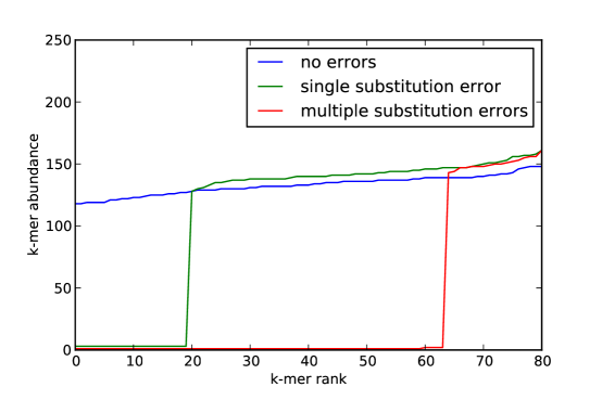
We may calculate a reference-free estimate of genome coverage by looking at the k-mer abundance distribution within individual reads. First, observe that k-mers, DNA words of a fixed length $k$, tend to have similar abundances within a read: this is a well-known property of k-mers that stems from each read originating from a single source molecule of DNA. The more times a region is sequenced, the higher the abundance of k-mers from that region would be. In the absence of errors, average k-mer abundance could be used as an estimate of the depth of coverage for a particular read (Figure 1, “no errors” line). However, when reads contain random substitution or indel errors from sequencing, the k-mers overlapping these errors will be of lower abundance; this feature is often used in k-mer based error correction approaches [24]. For example, a single substitution will introduce $k$ low-abundance k-mers within a read. (Figure 1, “single substitution error” line). However, for small $k$ and reads of length $L$ where $L>3k-1$, a single substitution error will not skew the median k-mer abundance. Only when multiple substitution errors are found in a single read will the median k-mer abundance be affected (Figure 1, “multiple substitution errors”).

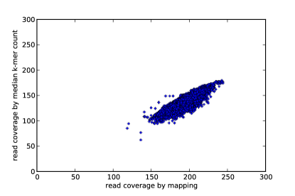
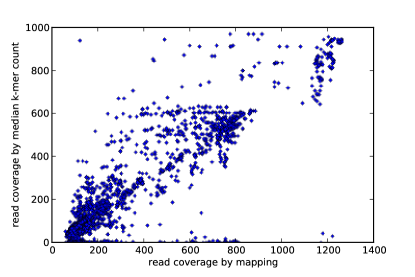
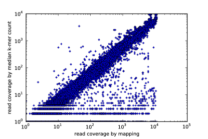
Using a fixed-memory CountMin Sketch data structure to count k-mers (see Methods and [27]), we find that median k-mer abundance correlates well with mapping-based coverage for artificial and real genomic data sets. There is a strong correlation between median k-mer abundance and mapping-based coverage both for simulated 100-base reads generated with 1% error from a 400kb artificial genome sequence ($r^{2}=0.79$; also see Figure 2a), as well as for real short-read data from E. coli ($r^{2}=0.80$, also see Figure 2b). This correlation also holds for simulated and real mRNAseq data: for simulated transcriptome data, $r^{2}=0.93$ (Figure 3a), while for real mouse transcriptome data, $r^{2}=0.90$ (Figure 3b). Thus the median k-mer abundance of a read correlates well with mapping-based estimates of read coverage.

Eliminating redundant reads reduces variation in sequencing depth

Deeply sequenced genomes contain many highly covered loci. For example, in a human genome sequenced to 100x average coverage, we would expect 50% or more of the reads to have a coverage greater than 100. In practice, we need many fewer of these reads to assemble the source locus.

Using the median k-mer abundance estimator discussed above, we can examine each read in the data set progressively to determine if it is high coverage. At the beginning of a shotgun data set, we would expect many reads to be entirely novel and have a low estimated coverage. As we proceed through the data set, however, average coverage will increase and many reads will be from loci that we have already sampled sufficiently.

Suppose we choose a coverage threshold $C$ past which we no longer wish to collect reads. If we only keep reads whose estimated coverage is less than $C$, and discard the rest, we will reduce the average coverage of the data set to $C$. This procedure is algorithmically straightforward to execute: we examine each read’s estimated coverage, and retain only those whose coverage is less than $C$. The following pseudocode provides one approach:

   for read in dataset:
      if estimated_coverage(read) < C:
         accept(read)
      else:
         discard(read)

where accepted reads contribute to the $\tt estimated\_coverage$ function. Note that for any data set with an average coverage $>2C$, this has the effect of discarding the majority of reads. Critically, low-coverage reads, especially reads from undersampled regions, will always be retained.

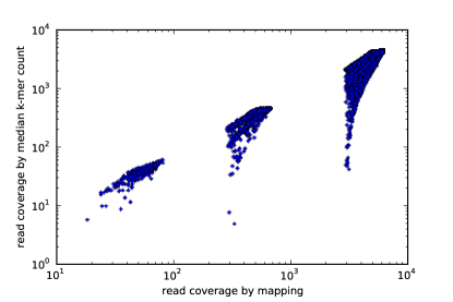
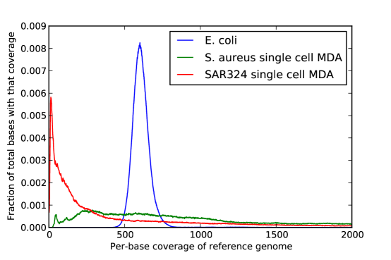
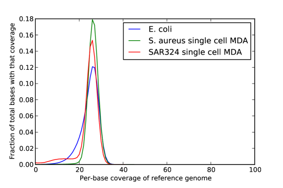
The net effect of this procedure, which we call digital normalization, is to normalize the coverage distribution of data sets. In Figure 4a, we display the estimated coverage of an E. coli genomic data set, a S. aureus single-cell MD-amplified data set, and an MD-amplified data set from an uncultured Deltaproteobacteria, calculated by mapping reads to the known or assembled reference genomes (see [19] for the data source). The wide variation in coverage for the two MDA data sets is due to the amplification procedure [28]. After normalizing to a k-mer coverage of 20, the high coverage loci are systematically shifted to an average mapping coverage of 26, while lower-coverage loci remain at their previous coverage. This smooths out coverage of the overall data set.

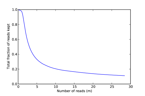
At what rate are sequences retained? For the E. coli data set, Figure 5 shows the fraction of sequences retained by digital normalization as a function of the total number of reads examined when normalizing to C=20 at k=20. There is a clear saturation effect showing that as more reads are examined, a smaller fraction of reads is retained; by 5m reads, approximately 50-100x coverage of E. coli, under 30% of new reads are kept. This demonstrates that as expected, only a small amount of novelty (in the form of either new information, or the systematic accumulation of errors) is being observed with increasing sequencing depth.

Digital normalization retains information while discarding both data and errors

The 1-2% per-base error rate of next-generation sequencers dramatically affect the total number of k-mers. For example, in the simulated genomic data of 200x, a 1% error rate leads to approximately 20 new k-mers for each error, yielding 20-fold more k-mers in the reads than are truly present in the genome (Table 1, row 1). This in turn dramatically increases the memory requirements for tracking and correcting k-mers [4]. This is a well-known problem with de Bruijn graph approaches, in which erroneous nodes or edges quickly come to dominate deep sequencing data sets.

When we perform digital normalization on such a data set, we eliminate the vast majority of these k-mers (Table 1, row 1). This is because we are accepting or rejecting entire reads; in going from 200x random coverage to 20x systematic coverage, we discard 80% of the reads containing 62% of the errors (Table 1, row 1). For reads taken from a skewed abundance distribution, such as with MDA or mRNAseq, we similarly discard many reads, and hence many errors (Table 1, row 2). In fact, in most cases the process of sequencing fails to recover more true k-mers (Table 1, middle column, parentheses) than digital normalization discards (Table 1, fourth column, parentheses).

The net effect of digital normalization is to retain nearly all real k-mers, while discarding the majority of erroneous k-mers – in other words, digital normalization is discarding data but not information. This rather dramatic elimination of erroneous k-mers is a consequence of the high error rate present in reads: with a 1% per-base substitution error rate, each 100-bp read will have an average of one substitution error. Each of these substitution errors will introduce up to $k$ erroneous k-mers. Thus, for each read we discard as redundant, we also eliminate an average of $k$ erroneous k-mers.

We may further eliminate erroneous k-mers by removing k-mers that are rare across the data set; these rare k-mers tend to result from substitution or indel errors [24]. We do this by first counting all the k-mers in the accepted reads during digital normalization. We then execute a second pass across the accepted reads in which we eliminate the 3’ ends of reads at low-abundance k-mers. Following this error reduction pass, we execute a second round of digital normalization (a third pass across the data set) that further eliminates redundant data. This three-pass protocol eliminates additional errors and results in a further decrease in data set size, at the cost of very few real k-mers in genomic data sets (Table 2).

Why use this three-pass protocol rather than simply normalizing to the lowest desired coverage in the first pass? We find that removing low-abundance k-mers after a single normalization pass to $C\approx 5$ removes many more real k-mers, because there will be many regions in the genome that by chance have yielded 5 reads with errors in them. If these erroneous k-mers are removed in the abundance-trimming step, coverage of the corresponding regions is eliminated. By normalizing to a higher coverage of 20, removing errors, and only then reducing coverage to 5, digital normalization can retain accurate reads for most regions. Note that this three-pass protocol is not considerably more computationally expensive than the single-pass protocol: the first pass discards the majority of data and errors, so later passes are less time and memory intensive than the first pass.

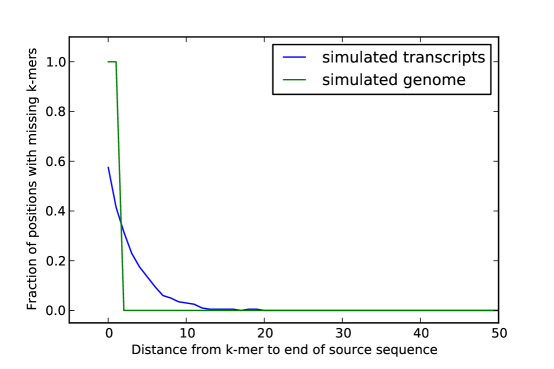
Interestingly, this three-pass protocol removed many more real k-mers from the simulated mRNAseq data than from the simulated genome – 351 of 48,100 (0.7%) real k-mers are lost from the mRNAseq, vs 4 of 399,981 lost (.000001%) from the genome (Table 2). While still only a tiny fraction of the total number of real k-mers, the difference is striking – the simulated mRNAseq sample loses k-mers at almost 1000-fold the rate of the simulated genomic sample. Upon further investigation, all but one of the lost k-mers were located within 20 bases of the ends of the source sequences; see Figure 6. This is because digital normalization cannot distinguish between erroneous k-mers and k-mers that are undersampled due to edge effects. In the case of the simulated genome, which was generated as one large chromosome, the effect is negligible, but the simulated transcriptome was generated as 100 transcripts of length 500. This added 99 end sequences over the genomic simulation, which in turn led to many more lost k-mers.

While the three-pass protocol is effective at removing erroneous k-mers, for some samples it may be too stringent. For example, the mouse mRNAseq data set contains only 100m reads, which may not be enough to thoroughly sample the rarest molecules; in this case the abundance trimming would remove real k-mers as well as erroneous k-mers. Therefore we used the single-pass digital normalization for the yeast and mouse transcriptomes. For these two samples we can also see that the first-pass digital normalization is extremely effective, eliminating essentially all of the erroneous k-mers (Table 1, rows 4 and 5.)

Digital normalization scales assembly of microbial genomes

We applied the three-pass digital normalization and error trimming protocol to three real data sets from Chitsaz et al (2011) [19]. The first pass of digital normalization was performed in 1gb of memory and took about 1 min per million reads. For all three samples, the number of reads remaining after digital normalization was reduced by at least 30-fold, while the memory and time requirements were reduced 10-100x.

Despite this dramatic reduction in data set size and computational requirements for assembly, both the E. coli and S. aureus assemblies overlapped with the known reference sequence by more than 98%. This confirms that little or no information was lost during the process of digital normalization; moreover, it appears that digital normalization does not significantly affect the assembly results. (Note that we did not perform scaffolding, since the digital normalization algorithm does not take into account paired-end sequences, and could mislead scaffolding approaches. Therefore, these results cannot directly be compared to those in Chitsaz et al. (2011) [19].)

The Deltaproteobacteria sequence also assembled well, with 98.8% sequence overlap with the results from Chitsaz et al. Interestingly, only 30kb of the sequence assembled with Velvet-SC in Chitsaz et al. (2011) was missing, while an additional 360kb of sequence was assembled only in the normalized samples. Of the 30kb of missing sequence, only 10% matched via TBLASTX to a nearby Deltaproteobacteria assembly, while more than 40% of the additional 360kb matched to the same Deltaproteobacteria sample. Therefore these additional contigs likely represents real sequence, suggesting that digital normalization is competitive with Velvet-SC in terms of sensitivity.

Digital normalization scales assembly of transcriptomes

We next applied single-pass digital normalization to published yeast and mouse mRNAseq data sets, reducing them to 20x coverage at k=20 [15]. Digital normalization on these samples used 8gb of memory and took about 1 min per million reads. We then assembled both the original and normalized sequence reads with Oases and Trinity, two de novo transcriptome assemblers (Table 4) [16, 15].

For both assemblers the computational resources necessary to complete an assembly were reduced (Table 4), but normalization had different effects on performance for the different samples. On the yeast data set, time and memory requirements were reduced significantly, as for Oases running on mouse. However, while Trinity’s runtime decreased by a factor of three on the normalized mouse data set, the memory requirements did not decrease significantly. This may be because the mouse transcriptome is 5-6 times larger than the yeast transcriptome, and so the mouse mRNAseq is lower coverage overall; in this case we would expect fewer errors to be removed by digital normalization.

The resulting assemblies differed in summary statistics (Table 5). For both yeast and mouse, Oases lost 5-10% of total transcripts and total bases when assembling the normalized data. However, Trinity gained transcripts when assembling the normalized yeast and mouse data, gaining about 1% of total bases on yeast and losing about 1% of total bases in mouse. Using a local-alignment-based overlap analysis (see Methods) we found little difference in sequence content between the pre- and post- normalization assemblies: for example, the normalized Oases assembly had a 98.5% overlap with the unnormalized Oases assembly, while the normalized Trinity assembly had a 97% overlap with the unnormalized Trinity assembly.

To further investigate the differences between transcriptome assemblies caused by digital normalization, we looked at the sensitivity with which long transcripts were recovered post-normalization. When comparing the normalized assembly to the unnormalized assembly in yeast, Trinity lost only 3% of the sequence content in transcripts greater than 300 bases, but 10% of the sequence content in transcripts greater than 1000 bases. However, Oases lost less than 0.7% of sequence content at 300 and 1000 bases. In mouse, we see the same pattern. This suggests that the change in summary statistics for Trinity is caused by fragmentation of long transcripts into shorter transcripts, while the difference for Oases is caused by loss of splice variants. Indeed, this loss of splice variants should be expected, as there are many low-prevalence splice variants present in deep sequencing data [29]. Interestingly, in yeast we recover more transcripts after digital normalization; these transcripts appear to be additional splice variants.

The difference between Oases and Trinity results show that Trinity is more sensitive to digital normalization than Oases: digital normalization seems to cause Trinity to fragment long transcripts. Why? One potential issue is that Trinity only permits k=26 for assembly, while normalization was performed at k=20; digital normalization may be removing 26-mers that are important for Trinity’s path finding algorithm. Alternatively, Trinity may be more sensitive than Oases to the change in coverage caused by digital normalization. Regardless, the strong performance of Oases on digitally normalized samples, as well as the high retention of k-mers (Table 1) suggests that the primary sequence content for the transcriptome remains present in the normalized reads, although it is recovered with different effectiveness by the two assemblers.

Discussion

Digital normalization dramatically scales de novo assembly

The results from applying digital normalization to read data sets prior to de novo assembly are extremely good: digital normalization reduces the computational requirements (time and memory) for assembly considerably, without substantially affecting the assembly results. It does this in two ways: first, by removing the majority of reads without significantly affecting the true k-mer content of the data set. Second, by eliminating these reads, digital normalization also eliminates sequencing errors contained within those reads, which otherwise would add significantly to memory usage in assembly [4].

Digital normalization also lowers computational requirements by eliminating most repetitive sequence in the data set. Compression-based approaches to graph storage have demonstrated that compressing repetitive sequence also effectively reduces memory and compute requirements [30, 11]. Note however that eliminating many repeats may also have its negatives (discussed below).

Digital normalization should be an effective preprocessing approach for most assemblers. In particular, the de Bruijn graph approach used in many modern assemblers relies on k-mer content, which is almost entirely preserved by digital normalization (see Tables 1 and 2) [2].

A general strategy for normalizing coverage

Digital normalization is a general strategy for systematizing coverage in shotgun sequencing data sets by using per-locus downsampling, albeit without any prior knowledge of reference loci. This yields considerable theoretical and practical benefits in the area of de novo sequencing and assembly.

In theoretical terms, digital normalization offers a general strategy for changing the scaling behavior of sequence assembly. Assemblers tend to scale poorly with the number of reads: in particular, de Bruijn graph memory requirements scale linearly with the size of the data set due to the accumulation of errors, although others have similarly poor scaling behavior (e.g. quadratic time in the number of reads) [2]. By calculating per-locus coverage in a way that is insensitive to errors, digital normalization converts genome assembly into a problem that scales with the complexity of the underlying sample - i.e. the size of the genome, transcriptome, or metagenome.

Digital normalization also provides a general strategy for applying online or streaming approaches to analysis of de novo sequencing data. The basic algorithm presented here is explicitly a single-pass or streaming algorithm, in which the entire data set is never considered as a whole; rather, a partial “sketch” of the data set is retained and used for progressive filtering. Online algorithms and sketch data structures offer significant opportunities in situations where data sets are too large to be conveniently stored, transmitted, or analyzed [31]. This can enable increasingly efficient downstream analyses. Digital normalization can be applied in any situation where the abundance of particular sequence elements is either unimportant or can be recovered more efficiently after other processing, as in assembly.

The construction of a simple, reference-free measure of coverage on a per-read basis offers opportunities to analyze coverage and diversity with an assembly-free approach. Genome and transcriptome sequencing is increasingly being applied to non-model organisms and ecological communities for which there are no reference sequences, and hence no good way to estimate underlying sequence complexity. The reference-free counting technique presented here provides a method for determining community and transcriptome complexity; it can also be used to progressively estimate sequencing depth.

More pragmatically, digital normalization also scales existing assembly techniques dramatically. The reduction in data set size afforded by digital normalization may also enable the application of more computationally expensive algorithms such as overlap-layout-consensus assembly approaches to short-read data. Overall, the reduction in data set size, memory requirements, and time complexity for contig assembly afforded by digital normalization could lead to the application of more complex heuristics to the assembly problem.

Digital normalization drops terminal k-mers and removes isoforms

Our implementation of digital normalization does discard some real information, including terminal k-mers and low-abundance isoforms. Moreover, we predict a number of other failure modes: for example, because k-mer approaches demand strict sequence identity, data sets from highly polymorphic organisms or populations will perform more poorly than data sets from low-variability samples. Digital normalization also discriminates against highly repetitive sequences. We note that these problems traditionally have been challenges for assembly strategies: recovering low-abundance isoforms from mRNAseq, assembling genomes from highly polymorphic organisms, and assembling across repeats are all difficult tasks, and improvements in these areas continue to be active areas of research [32, 33, 34]. Using an alignment-based approach to estimating coverage, rather than a k-mer based approach, could provide an alternative implementation that would improve performance on errors, splice variants, and terminal k-mers. Our current approach also ignores quality scores; a “q-mer” counting approach as in Quake, in which k-mer counts are weighted by quality scores, could easily be adapted [24].

Another concern for normalizing deep sequencing data sets is that, with sufficiently deep sequencing, sequences with many errors will start to accrue. This underlies the continued accumulation of sequence data for E. coli observed in Figure 5. Assemblers may be unable to distinguish between this false sequence and the error-free sequences, for sufficiently deep data sets. This accumulation of erroneous sequences is again caused by the use of k-mers to detect similarity, and is one reason why exploring local alignment approaches (discussed below) may be a good future direction.

Applying assembly algorithms to digitally normalized data

The assembly problem is challenging for several reasons: many formulations are computationally complex (NP-hard), and practical issues of both genome content and sequencing, such as repetitive sequence, polymorphisms, short reads and high error rates, challenge assembly approaches [35]. This has driven the development of heuristic approaches to resolving complex regions in assemblies. Several of these heuristic approaches use the abundance information present in the reads to detect and resolve repeat regions; others use pairing information from paired-end and mate-pair sequences to resolve complex paths. Digital normalization aggressively removes abundance information, and we have not yet adapted it to paired-end sequencing data sets; this could and should affect the quality of assembly results! Moreover, it is not clear what effect different coverage (C) and k-mer (k) values have on assemblers. In practice, for at least one set of k-mer size $k$ and normalized coverage $C$ parameters, digital normalization seems to have little negative effect on the final assembled contigs. Further investigation of the effects of varying $k$ and $C$ relative to specific assemblers and assembler parameters will likely result in further improvements in assembly quality.

A more intriguing notion than merely using digital normalization as a pre-filter is to specifically adapt assembly algorithms and protocols to digitally normalized data. For example, the reduction in data set size afforded by digital normalization may make overlap-layout-consensus approaches computationally feasible for short-read data [2]. Alternatively, the quick and inexpensive generation of contigs from digitally normalized data could be used prior to a separate scaffolding step, such as those supported by SGA and Bambus2 [14, 36]. Digital normalization offers many future directions for improving assembly.

Conclusions

Digital normalization is an effective demonstration that much of short-read shotgun sequencing is redundant. Here we have shown this by normalizing samples to 5-20x coverage while recovering complete or nearly complete contig assemblies. Normalization is substantially different from uniform downsampling: by doing downsampling in a locus-specific manner, we retain low coverage data. Previously described approaches to reducing sampling variation rely on ad hoc parameter measures and/or an initial round of assembly and have not been shown to be widely applicable [20, 21].

We have implemented digital normalization as a prefilter for assembly, so that any assembler may be used on the normalized data. Here we have only benchmarked a limited set of assemblers – Velvet, Oases, and Trinity – but in theory digital normalization should apply to any assembler. De Bruijn and string graph assemblers such as Velvet, SGA, SOAPdenovo, Oases, and Trinity are especially likely to work well with digital normalized data, due to the underlying reliance on k-mer overlaps in these assemblers.

Digital normalization is widely applicable and computationally convenient

Digital normalization can be applied de novo to any shotgun data set. The approach is extremely computationally convenient: the runtime complexity is linear with respect to the data size, and perhaps more importantly it is single-pass: the basic algorithm does not need to look at any read more than once. Moreover, because reads accumulate sub-linearly, errors do not accumulate quickly and overall memory requirements for digital normalization should grow slowly with data set size. Note also that while the algorithm presented here is not perfectly parallelizable, efficient distributed k-mer counting is straightforward and it should be possible to scale digital normalization across multiple machines [37].

The first pass of digital normalization is implemented as an online streaming algorithm in which reads are examined once. Streaming algorithms are useful for solving data analysis problems in which the data are too large to easily be transmitted, processed, or stored. Here, we implement the streaming algorithm using a fixed memory data “sketch” data structure, CountMin Sketch. By combining a single-pass algorithm with a fixed-memory data structure, we provide a data reduction approach for sequence data analysis with both (linear) time and (constant) memory guarantees. Moreover, because the false positive rate of the CountMin Sketch data structure is well understood and easy to predict, we can provide data quality guarantees as well. These kinds of guarantees are immensely valuable from an algorithmic perspective, because they provide a robust foundation for further work [31]. The general concept of removing redundant data while retaining information underlies “lossy compression”, an approach used widely in image processing and video compression. The concept of lossy compression has broad applicability in sequence analysis. For example, digital normalization could be applied prior to homology search on unassembled reads, potentially reducing the computational requirements for e.g. BLAST and HMMER without loss of sensitivity. Digital normalization could also help merge multiple different read data sets from different read technologies, by discarding entirely redundant sequences and retaining only sequences containing “new” information. These approaches remain to be explored in the future.

Methods

All links below are available electronically through ged.msu.edu/papers/2012-diginorm/, in addition to the archival locations provided.

Data sets

The E. coli, S. aureus, and Deltaproteobacteria data sets were taken from Chitsaz et al. [19], and downloaded from bix.ucsd.edu/projects/singlecell/. The mouse data set was published by Grabherr et al. [15] and downloaded from trinityrnaseq.sf.net/. All data sets were used without modification. The complete assemblies, both pre- and post-normalization, for the E. coli, S. aureus, the uncultured Deltaproteobacteria, mouse, and yeast data sets are available from ged.msu.edu/papers/2012-diginorm/.

The simulated genome and transcriptome were generated from a uniform AT/CG distribution. The genome consisted of a single chromosome 400,000 bases in length, while the transcriptome consisted of 100 transcripts of length 500. 100-base reads were generated uniformly from the genome to an estimated coverage of 200x, with a random 1% per-base error. For the transcriptome, 1 million reads of length 100 were generated from the transcriptome at relative expression levels of 10, 100, and 1000, with transcripts assigned randomly with equal probability to each expression group; these reads also had a 1% per-base error.

Scripts and software

All simulated data sets and all analysis summaries were generated by Python scripts, which are available at github.com/ged-lab/2012-paper-diginorm/. Digital normalization and k-mer analyses were performed with the khmer software package, written in C++ and Python, available at github.com/ged-lab/khmer/, tag ’2012-paper-diginorm’. khmer also relies on the screed package for loading sequences, available at github.com/ged-lab/screed/, tag ’2012-paper-diginorm’. khmer and screed are Copyright (c) 2010 Michigan State University, and are free software available for distribution, modification, and redistribution under the BSD license.

Mapping was performed with bowtie v0.12.7 [38]. Genome assembly was done with velvet 1.2.01 [9]. Transcriptome assembly was done with velvet 1.1.05/oases 0.1.22 and Trinity, head of branch on 2011.10.29. Graphs and correlation coefficients were generated using matplotlib v1.1.0, numpy v1.7, and ipython notebook v0.12 [39]. The ipython notebook file and data analysis scripts necessary to generate the figures are available at github.com/ged-lab/2012-paper-diginorm/.

Analysis parameters

The khmer software uses a CountMin Sketch data structure to count k-mers, which requires a fixed memory allocation [27]. In all cases the memory usage was fixed such that the calculated false positive rate was below 0.01. By default k was set to 20.

Genome and transcriptome coverage was calculated by mapping all reads to the reference with bowtie (-a --best --strata) and then computing the per-base coverage in the reference. Read coverage was computed by then averaging the per-base reference coverage for each position in the mapped read; where reads were mapped to multiple locations, a reference location was chosen randomly for computing coverage. Median k-mer counts were computed with khmer as described in the text. Artificially high counts resulting from long stretches of Ns were removed after the analysis. Correlations between median k-mer counts and mapping coverage were computed using numpy.corrcoef; see calc-r2.py script.

Normalization and assembly parameters

For Table 3, the assembly k parameter for Velvet was k=45 for E. coli; k=41 for S. aureus single cell; and k=39 for Deltaproteobacteria single cell. Digital normalization on the three bacterial samples was done with -N 4 -x 2.5e8 -k 20, consuming 1gb of memory. Post-normalization k parameters for Velvet assemblies were k=37 for E. coli, k=27 for S. aureus, and k=27 for Deltaproteobacteria. For Table 4, the assembly k parameter for Oases was k=21 for yeast and k=23 for mouse. Digital normalization on both mRNAseq samples was done with -N 4 -x 2e9 -k 20, consuming 8gb of memory. Assembly of the single-pass normalized mRNAseq was done with Oases at k=21 (yeast) and k=19 (mouse).

Assembly overlap and analysis

Assembly overlap was computed by first using NCBI BLASTN to build local alignments for two assemblies, then filtering for matches with bit scores $>$ 200, and finally computing the fraction of bases in each assembly with at least one alignment. Total fractions were normalized to self-by-self BLASTN overlap identity to account for BLAST-specific sequence filtering. TBLASTX comparison of the Deltaproteobacteria SAR324 sequence was done against another assembled SAR324 sequence, acc AFIA01000002.1.

Compute requirement estimation

Execution time was measured using real time from Linux bash ’time’. Peak memory usage was estimated either by the ’memusg’ script from stackoverflow.com, peak-memory-usage-of-a-linux-unix-process, included in the khmer repository; or by the Torque queuing system monitor, for jobs run on MSU’s HPC system. While several different machines were used for analyses, comparisons between unnormalized and normalized data sets were always done on the same machine.

Figure Legends

Figure 1: Representative rank-abundance distributions for 20-mers from 100-base reads with no errors, a read with a single substitution error, and a read with multiple substitution errors.

Figure 2: Mapping and k-mer coverage measures correlate for simulated genome data and a real E. coli data set (5m reads). Simulated data $r^{2}=0.79$; E. coli $r^{2}=0.80$.

Figure 3: Mapping and k-mer coverage measures correlate for simulated transcriptome data as well as real mouse transcriptome data. Simulated data $r^{2}=0.93$; mouse transcriptome $r^{2}=0.90$.

Figure 4: Coverage distribution of three microbial genome samples, calculated from mapped reads (a) before and (b) after digital normalization (k=20, C=20).

Figure 5: Fraction of reads kept when normalizing the E. coli dataset to C=20 at k=20.

Figure 6: K-mers at the ends of sequences are lost during digital normalization.

Tables

Table 1: Digital normalization to C=20 removes many erroneous k-mers from sequencing data sets. Numbers in parentheses indicate number of true k-mers lost at each step, based on reference.

Data set	True 20-mers	20-mers in reads	20-mers at C=20	% reads kept
Simulated genome	399,981	8,162,813	3,052,007 (-2)	19%
Simulated mRNAseq	48,100	2,466,638 (-88)	1,087,916 (-9)	4.1%
E. coli genome	4,542,150	175,627,381 (-152)	90,844,428 (-5)	11%
Yeast mRNAseq	10,631,882	224,847,659 (-683)	10,625,416 (-6,469)	9.3%
Mouse mRNAseq	43,830,642	709,662,624 (-23,196)	43,820,319 (-13,400)	26.4%

Table 2: Three-pass digital normalization removes most erroneous k-mers. Numbers in parentheses indicate number of true k-mers lost at each step, based on known reference.

Data set	True 20-mers	20-mers in reads	20-mers remaining	% reads kept
Simulated genome	399,981	8,162,813	453,588 (-4)	5%
Simulated mRNAseq	48,100	2,466,638 (-88)	182,855 (-351)	1.2%
E. coli genome	4,542,150	175,627,381 (-152)	7,638,175 (-23)	2.1%
Yeast mRNAseq	10,631,882	224,847,659 (-683)	10,532,451 (-99,436)	2.1%
Mouse mRNAseq	43,830,642	709,662,624 (-23,196)	42,350,127 (-1,488,380)	7.1%

Table 3: Three-pass digital normalization reduces computational requirements for contig assembly of genomic data.

Data set	N reads pre/post	Assembly time pre/post	Assembly memory pre/post
E. coli	31m / 0.6m	1040s / 63s (16.5x)	11.2gb / 0.5 gb (22.4x)
S. aureus single-cell	58m / 0.3m	5352s / 35s (153x)	54.4gb / 0.4gb (136x)
Deltaproteobacteria single-cell	67m / 0.4m	4749s / 26s (182.7x)	52.7gb / 0.4gb (131.8x)

Table 4: Single-pass digital normalization to C=20 reduces computational requirements for transcriptome assembly.

Data set	N reads pre/post	Assembly time pre/post	Assembly memory pre/post
Yeast (Oases)	100m / 9.3m	181 min / 12 min (15.1x)	45.2gb / 8.9gb (5.1x)
Yeast (Trinity)	100m / 9.3m	887 min / 145 min (6.1x)	31.8gb / 10.4gb (3.1x)
Mouse (Oases)	100m / 26.4m	761 min/ 73 min (10.4x)	116.0gb / 34.6gb (3.4x)
Mouse (Trinity)	100m / 26.4m	2297 min / 634 min (3.6x)	42.1gb / 36.4gb (1.2x)

Table 5: Digital normalization has assembler-specific effects on transcriptome assembly.

Data set	Contigs $>$ 300	Total bp $>$ 300	Contigs $>$ 1000	Total bp $>$ 1000
Yeast (Oases)	12,654 / 9,547	33.2mb / 27.7mb	9,156 / 7,345	31.2mb / 26.4mb
Yeast (Trinity)	10,344 / 12,092	16.2mb / 16.5mb	5,765 / 6,053	13.6 mb / 13.1mb
Mouse (Oases)	57,066 / 49,356	98.1mb / 84.9mb	31,858 / 27,318	83.7mb / 72.4mb
Mouse (Trinity)	50,801 / 61,242	79.6 mb / 78.8mb	23,760 / 24,994	65.7mb / 59.4mb

References

- 1. Metzker M (2010) Sequencing technologies - the next generation. Nat Rev Genet 11: 31-46.
- 2. Miller J, Koren S, Sutton G (2010) Assembly algorithms for next-generation sequencing data. Genomics 95: 315-27.
- 3. Gnerre S, Maccallum I, Przybylski D, Ribeiro F, Burton J, et al. (2011) High-quality draft assemblies of mammalian genomes from massively parallel sequence data. Proc Natl Acad Sci U S A 108: 1513-8.
- 4. Conway T, Bromage A (2011) Succinct data structures for assembling large genomes. Bioinformatics 27: 479-86.
- 5. Sboner A, Mu X, Greenbaum D, Auerbach R, Gerstein M (2011) The real cost of sequencing: higher than you think! Genome Biol 12: 125.
- 6. Stein L (2010) The case for cloud computing in genome informatics. Genome Biol 11: 207.
- 7. Trapnell C, Salzberg S (2009) How to map billions of short reads onto genomes. Nat Biotechnol 27: 455-7.
- 8. Simpson J, Wong K, Jackman S, Schein J, Jones S, et al. (2009) Abyss: a parallel assembler for short read sequence data. Genome Res 19: 1117-23.
- 9. Zerbino D, Birney E (2008) Velvet: algorithms for de novo short read assembly using de bruijn graphs. Genome Res 18: 821-9.
- 10. Li Y, Hu Y, Bolund L, Wang J (2010) State of the art de novo assembly of human genomes from massively parallel sequencing data. Hum Genomics 4: 271-7.
- 11. Simpson J, Durbin R (2012) Efficient de novo assembly of large genomes using compressed data structures. Genome Res 22: 549-56.
- 12. Iqbal Z, Caccamo M, Turner I, Flicek P, McVean G (2012) De novo assembly and genotyping of variants using colored de bruijn graphs. Nat Genet 44: 226-32.
- 13. Compeau P, Pevzner P, Tesler G (2011) How to apply de bruijn graphs to genome assembly. Nat Biotechnol 29: 987-91.
- 14. Simpson J, Durbin R (2010) Efficient construction of an assembly string graph using the fm-index. Bioinformatics 26: i367-73.
- 15. Grabherr M, Haas B, Yassour M, Levin J, Thompson D, et al. (2011) Full-length transcriptome assembly from rna-seq data without a reference genome. Nat Biotechnol 29: 644-52.
- 16. Schulz M, Zerbino D, Vingron M, Birney E (2012) Oases: robust de novo rna-seq assembly across the dynamic range of expression levels. Bioinformatics 28: 1086-92.
- 17. Namiki T, Hachiya T, Tanaka H, Sakakibara Y (2011) MetaVelvet: An extension of Velvet assembler to de novo metagenome assembly from short sequence reads. ACM Conference on Bioinformatics, Computational Biology and Biomedicine .
- 18. Peng Y, Leung H, Yiu S, Chin F (2011) Meta-idba: a de novo assembler for metagenomic data. Bioinformatics 27: i94-101.
- 19. Chitsaz H, Yee-Greenbaum J, Tesler G, Lombardo M, Dupont C, et al. (2011) Efficient de novo assembly of single-cell bacterial genomes from short-read data sets. Nat Biotechnol 29: 915-21.
- 20. Rodrigue S, Malmstrom R, Berlin A, Birren B, Henn M, et al. (2009) Whole genome amplification and de novo assembly of single bacterial cells. PLoS One 4: e6864.
- 21. Woyke T, Sczyrba A, Lee J, Rinke C, Tighe D, et al. (2011) Decontamination of mda reagents for single cell whole genome amplification. PLoS One 6: e26161.
- 22. Medvedev P, Scott E, Kakaradov B, Pevzner P (2011) Error correction of high-throughput sequencing datasets with non-uniform coverage. Bioinformatics 27: i137-41.
- 23. Chaisson M, Pevzner P, Tang H (2004) Fragment assembly with short reads. Bioinformatics 20: 2067-74.
- 24. Kelley D, Schatz M, Salzberg S (2010) Quake: quality-aware detection and correction of sequencing errors. Genome Biol 11: R116.
- 25. Bonaldo M, Lennon G, Soares M (1996) Normalization and subtraction: two approaches to facilitate gene discovery. Genome Res 6: 791-806.
- 26. Soares M, Bonaldo M, Jelene P, Su L, Lawton L, et al. (1994) Construction and characterization of a normalized cdna library. Proc Natl Acad Sci U S A 91: 9228-32.
- 27. Cormode G, Muthukrishnan S (2004) An improved data stream summary: the count-min sketch, and its applications. Journal of Algorithms .
- 28. Spits C, Caignec CL, Rycke MD, Haute LV, Steirteghem AV, et al. (2006) Whole-genome multiple displacement amplification from single cells. Nat Protoc 1: 1965-70.
- 29. Pickrell J, Pai A, Gilad Y, Pritchard J (2010) Noisy splicing drives mrna isoform diversity in human cells. PLoS Genet 6: e1001236.
- 30. Pinho A, Pratas D, Garcia S (2012) Green: a tool for efficient compression of genome resequencing data. Nucleic Acids Res 40: e27.
- 31. Muthukrishnan S (2005) Data streams: algorithms and applications. Foundations and trends in theoretical computer science. Now Publishers. URL http://books.google.com/books?id=415loiMd_c0C.
- 32. Do H, Choi K, Preparata F, Sung W, Zhang L (2008) Spectrum-based de novo repeat detection in genomic sequences. J Comput Biol 15: 469-87.
- 33. Novak P, Neumann P, Macas J (2010) Graph-based clustering and characterization of repetitive sequences in next-generation sequencing data. BMC Bioinformatics 11: 378.
- 34. Gu W, Castoe T, Hedges D, Batzer M, Pollock D (2008) Identification of repeat structure in large genomes using repeat probability clouds. Anal Biochem 380: 77-83.
- 35. Nagarajan N, Pop M (2009) Parametric complexity of sequence assembly: theory and applications to next generation sequencing. J Comput Biol 16: 897-908.
- 36. Koren S, Treangen T, Pop M (2011) Bambus 2: scaffolding metagenomes. Bioinformatics 27: 2964-71.
- 37. Schatz M (2009) Cloudburst: highly sensitive read mapping with mapreduce. Bioinformatics 25: 1363-9.
- 38. Langmead B, Trapnell C, Pop M, Salzberg S (2009) Ultrafast and memory-efficient alignment of short dna sequences to the human genome. Genome Biol 10: R25.
- 39. Pérez F, Granger BE (2007) IPython: a System for Interactive Scientific Computing. Comput Sci Eng 9: 21-29.