On the Stability of Contention Resolution Diversity Slotted ALOHA

Abstract

In this paper a Time Division Multiple Access (TDMA) based Random Access (RA) channel with Successive Interference Cancellation (SIC) is considered for a finite user population and reliable retransmission mechanism on the basis of Contention Resolution Diversity Slotted ALOHA (CRDSA). A general mathematical model based on Markov Chains is derived which makes it possible to predict the stability regions of SIC-RA channels, the expected delays in equilibrium and the selection of parameters for a stable channel configuration. Furthermore the model enables the estimation of the average time before reaching instability. The presented model is verified against simulations and numerical results are provided for comparison of the stability of CRDSA versus the stability of traditional Slotted ALOHA (SA). The presented results show that CRDSA has not only a high gain over SA in terms of throughput but also in its stability.

I Introduction

While the application of RA techniques for data transmissions is appealing in many application scenarios such as sensor networks, signalling or unpredictable and bursty low duty cycle user traffic, often concerns are expressed about the limitations in terms of spectral efficiency and the risk of RA channel instability, leading to a zero throughput and a correspondingly infinite transmission delay. While recently significant improvements of the spectral efficiency have been achieved by introducing SIC and coding techniques (e.g. [1], [2] and [3]), the stability behaviour of these new schemes has not been fully analyzed yet. In [4] a first analysis of the stability of CRDSA as SIC representative was done and a mathematical model for the prediction of the channel stability was derived, which is used as baseline for the work presented in this paper and therefore recalled in the following.

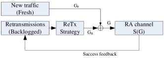
Figure 1: Feedback loop of a RA channel.

The source of channel instability in a RA channel is the natural occurrence of collisions among the packet transmission and the presence of mechanisms which attempt the retransmission of lost packets. In principle collided packets could be simply discarded, but doing so would adversely affect the Quality of Service (QoS) experienced by the user or may be entirely unacceptable for critical signalling information, such as log-on messages. RA schemes thus usually attempt to retransmit the lost packets, either until they are successfully received or until a maximum number of retransmissions has been reached. In order to make retransmissions possible, the users need to receive feedback whether their transmission attempt was successful, e.g., by means of acknowledgements. The instantaneous throughput of the RA channel $S(G)$ is then dependent on the total load $G$, being the sum of the load due to new transmissions $G_{F}$ and the load due to retransmissions $G_{B}$. In this sense the RA channel forms a feedback loop as is illustrated in Fig. 1. It is an inherent property of closed-loop feedback systems, that the feedback can lead to amplifying self-excitation. Here this results in an increase of the overall load due to the additional retransmissions.

The throughput curves of ALOHA, SA [5], and CRDSA [1] all have in common that for increasing load $G$ the throughput $S(G)$ first increases until reaching a maximum throughput $S_{max}$. For further increasing load, $S(G)$ decreases again and asymptotically approaches zero.

If due to retransmission attempts of lost packets the total load exceeds a critical threshold, then even more packets experience a collision and get lost, resulting in an even higher retransmission load. In the end the channel is driven into total saturation in the area of having very high load and very low throughput. To reduce this amplification effect a retransmission strategy is used, which shall limit the load due to retransmissions and reduce the risk of getting more collisions (see Fig. 1). Many different retransmission strategies that try to achieve this goal are known from literature. In [6] the selection of the time of retransmission with uniform probability within a parameterizable interval $t\in[0,\,...,\,K]$ is proposed. In [5] a strategy is described where the decision for a retransmission attempt is taken with a probability $p_{r}$ in every slot (for SA) resulting in a geometric distribution. In [7] the selection of the retransmission time from an interval, which grows exponentially with every collision (Binary Exponential Backoff), is proposed. Finally the so called splitting algorithms (see e.g., [5], [8]) iteratively split the set of collided users into two sets and stabilize the system this way. Furthermore two different types of user population are distinguished, finite and infinite user populations. For a finite user population, every user that experienced a collision is backlogged, which means that he is not generating any new traffic until the collided packet has been successfully transmitted. The infinite user population on the other hand refers to either an infinite number of users or a finite number of users that generate new traffic independently of whether another retransmission is still pending or not. While some retransmission strategies assume a visibility of the channel activities by all users, here we assume that every user has no instant visibility of other users activity (as is the case in satellite systems with directive links and long propagation delays) and only receives feedback about the success of his own transmission attempt from the receiving end system. The retransmission mechanisms using a uniform and geometric retransmission probability have in common that the probability of retransmission is a fixed parameter and does not change dynamically. For the binary exponential backoff and tree splitting algorithm, the actual retransmission probability may change over time dependent on the situation. In the remainder of this paper the focus is on a geometrically distributed retransmission mechanism, since it was shown in [9] that the channel performance of SA is mainly dependent on the average retransmission delay and largely independent of the retransmission probability distribution.

II Review of SIC-based Random Access Techniques

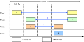
Figure 2: SIC principle of CRDSA. Numbers at arrows indicate the step in the iteration process.

Over the last years the recently regained popularity of RA schemes resulted in the definition of new RA protocols. In particular a recent enhancement of the SA protocol, named CRDSA [1], [10], using SIC techniques over a set of slots (denoted frame) to improve the throughput and Packet Loss Rate (PLR) behaviour of SA, has been studied showing an impressive gain over SA increasing the maximum throughput from $S_{max,SA}=0.36\frac{pkt}{slot}$ to $S_{max,CRDSA}=0.55\frac{pkt}{slot}$. Up to now however the consequences for the system stability of this new access scheme have not been analyzed yet. The fundamental concept of CRDSA is to generate a replica burst for every transmission burst within a set of $N_{S}$ slots, called frame, see also Fig. 2. While the generation of a redundant copy of a burst is similar to previous proposals such as Diversity Slotted ALOHA (DSA) [11], the fundamental difference here is that every burst contains a pointer to the location of its replica. In case a clean replica arrives, meaning that the burst could be decoded and received successfully, the channel is estimated from it and the interference that this burst introduces to other users is removed for all replica-burst locations.

In the example in Fig. 2 the first burst of user 1 is received successfully since not interfered. As consequence of the SIC process, the interference that the replica of user 1 introduces to the second burst of user 2 is removed so that this burst of user 2 can be decoded in the next round. This process is then iteratively repeated. In the example in Fig. 2 all replicas can be recovered this way.

II-A Characterization of the Packet Loss Rate in CRDSA

For classical SA, the necessary condition to have a successful reception is that only a single transmission must occur in a timeslot, otherwise the burst is lost. Let us denote by $M$ the total user population of the system and $p_{0}$ the probability that a user attempts a transmission in a time slot, then the probability that a user successfully receives a packet gets $p_{succ,SA}=p_{0}\cdot(1-p_{0})^{M-1}$. Increasing the overall number of users $M\to\infty$, the totally transmitted packets can be modeled as Poisson process with arrival rate $\lambda$ [12]. The probability for a successful transmission then results in the well known equation $p_{succ,SA}=\lambda\cdot T_{p}\cdot e^{-\lambda\cdot T_{p}}$, whereas $T_{p}$ denotes the slot duration. This simple closed form expression is conveniently suited to describe the throughput surfaces, which are used for the stability investigation done e.g., by Kleinrock [13]. The preconditions in CRDSA are however different due to the iterative SIC process. As was shown by Liva in [2] and [14], the SIC process can be interpreted as an erasure decoding process in a bipartite graph, such as for Low Density Parity Check Codes (LDPC) codes [15]. For this purpose, every slot in a frame is represented as a sum node and every transmitted burst by a burst node. The edges in the graph then connect the burst nodes to the sum nodes. In [2] an expression for the average erasure probabilities for every iteration are derived for the asymptotic case of infinitely long frames, resulting in an upper bound of the achievable throughput. An expression for neither the exact nor the average erasure probabilities in a non-asymptotic case with finite frame lengths however can be expressed accurately by these bounds or another closed form expression. For this reason the stability analysis in this work relies on simulated CRDSA packet success probabilities and throughput for the case of having one additional replica (degree $d=2$), a frame consisting of $N_{S}=100$ slots and a limitation of the number of SIC iterations to $I_{max}=10$. The presented framework is however flexible to be used as well for other configurations of CRDSA, always requiring only that the average throughput curve is known.

II-B Stability Definition

The issue of stability in RA systems was already identified in the very early days of the ALOHA proposal. Abramson [16] and Roberts [17] both addressed this issue for plain ALOHA. After the evolution of ALOHA towards SA, many publications have dealt with the investigation of the stability behaviour of SA, for instance [5], [18], [12] and [13]. Stability is commonly defined as the ability of a system to maintain equilibrium or return to the initial state after experiencing a distortion. In the context of RA, the term stability is used in different ways in literature. In the definition given by Abramson in [16], the ALOHA channel was defined instable if the average number of retransmissions becomes unbounded. Within [5] a channel was defined stable if the expected delay per packet is finite. Kleinrock defined in [13] a channel as stable if the SA equilibrium contour (i.e., throughput is equal to the channel input rate) is nontangentially intersected by the load line in exactly one place. In the strict mathematical definition of stability of autonomous systems, this corresponds to a sufficient condition for a global equilibrium point. In the terminology used by Kleinrock, a SA channel is instable if the load line intersects the equilibrium contour in more than one point. In the mathematical sense also then the system can have a locally stable equilibrium point, so the definition of stability by Kleinrock refers to the criterion of having a single globally stable equilibrium point. In the remainder of this work, the definitions given in [13] are followed also here, meaning that a channel is denoted as stable if it has a single globally stable equilibrium point and instable otherwise.

III Stability in CRDSA

Within this section, the derivation of a Markov model for a finite user population is described and the mathematical formulations for throughput and drift are derived, which form the core of the stability framework presented afterwards. This section concludes with a stability analysis for a representative CRDSA configuration.

Let the RA channel under consideration be populated by a total of $M$ users (finite user population). Every user resides either in a so called fresh (F) state or backlogged (B) state. In the beginning all $M$ users are in state F. Every user in state F attempts a new transmission in the current frame with probability $p_{0}$. It is further assumed that all users receive feedback about the success of their transmission at the end of a frame. In case the transmission attempt was successful, the user remains in state F. In case a packet is lost, the user enters state B. A user in state B attempts a retransmission of the lost packet with probability $p_{r}$ in the current frame. In case the retransmission is successful the user then returns to state F, otherwise the user remains in state B. Let $X_{\alpha}^{l}$ denote the number of users in state $\alpha\in\left\{F,B\right\}$ in frame $l$, then the discrete-time Markov chain can be fully described by either $X_{B}^{l}$ or $X_{F}^{l}$, since both are connected by $X_{F}^{l}=M-X_{B}^{l}$. In the following $X_{B}^{l}$ is chosen as the Markov state variable. Given the initial state $X_{B}^{0}=0$ and the state transition probability $P(x^{\prime}|x)$, which is the probability to move within one frame from backlog state $x$ to state $x^{\prime}$, the Markov chain is then fully described. One major difference to the SA analysis done by Kleinrock is that the backlog state for SA can at maximum decrease by 1 user per slot (otherwise there would be a collision), while the backlog state $X_{B}$ for CRDSA can decrease by $[1,\,\ldots,\,X_{B}]$ in a frame. Since no closed form expression for the success probability of a user in CRDSA is known in literature, the probability $q_{d,N_{s},I_{\text{max}}}(\tau,\upsilon)$ is introduced, which is the probability that out of $\tau$ users who attempt a transmission in the frame exactly $\upsilon$ users are successful. The success probability $q$ is dependent on the CRDSA configuration, consisting of the repetition degree $d$, the number of slots in the frame $N_{s}$ and the maximum number of iterations $I_{max}$. Here, this probability was derived numerically by simulations and averaging over the results for every offered load $G$. For sake of simplicity, the subscripts will be omitted in the following, using $q(\tau,\upsilon)$. When changing state, let $\upsilon_{l}$ be a random variable denoting the number of successful transmissions in frame $l$, $\varphi_{l}$ a random variable denoting the number of fresh transmission attempts in the frame and $\rho_{l}$ the number of retransmission attempts in a frame.

Let $FS_{l}$ denote the number of fresh users, which transmit successfully in frame $l$. Let $FU_{l}$ be the number of fresh users who attempted a transmission but were unsuccessful. In the same way, $BS_{l}$ denominates all backlogged users who attempt a retransmission and were successful and $BU_{l}$ those backlogged users, whose retransmission attempt was unsuccessful. The following equations (1)-(3) can be derived:

$$\varphi_{l}=FS_{l}+FU_{l},$$ (1)

$$\rho_{l}=BS_{l}+BU_{l},$$ (2)

$$\upsilon_{l}=FS_{l}+BS_{l}.$$ (3)

The joint probability mass function, conditioned on state $X^{l}=x_{B}$ is then given by Eq. (4).

$$P(\varphi,\rho,\upsilon|x_{B})={}$$ (4)

$${}=\binom{x_{F}}{\varphi}p_{0}^{\varphi}(1-p_{0})^{x_{F}-\varphi}\cdot\binom{x_{B}}{\rho}p_{r}^{\,\rho}(1-p_{r})^{x_{B}-\rho}$$

$${}\qquad\cdot q(\varphi+\rho,\upsilon)=$$

$${}=\binom{M-x_{B}}{\varphi}p_{0}^{\varphi}(1-p_{0})^{M-x_{B}-\varphi}$$

$${}\qquad\cdot\binom{x_{B}}{\rho}p_{r}^{\,\rho}(1-p_{r})^{x_{B}-\rho}$$

$${}\qquad\cdot q(\varphi+\rho,\upsilon).$$

With Eqs. (1)-(3) the change in number of backlogged users $\Delta x_{B}=x_{B,l+1}-x_{B,l}=x_{B}^{\prime}-x_{B}=FU-BS$ can be easily reformulated into:

$$\upsilon=\varphi+x_{B}-x_{B}^{\prime}$$ (5)

The state transition probability $P(x^{\prime}_{B}|x_{B})$ can then be formulated by combining (4) and (5) into (6):

$$P(x^{\prime}_{B}|x_{B})={}$$ (6)

$${}=\sum_{\varphi,\rho}P(\varphi,\rho,\varphi+x_{B}-x^{\prime}_{B}|x_{B})=$$

$${}=\sum_{\varphi,\rho}\binom{M-x_{B}}{\varphi}p_{0}^{\varphi}(1-p_{0})^{M-x_{B}-\varphi}$$

$${}\qquad\cdot\,\binom{x_{B}}{\rho}p_{r}^{\,\rho}(1-p_{r})^{x_{B}-\rho}$$

$${}\qquad\cdot q(\varphi+\rho,\varphi+x_{B}-x^{\prime}_{B}).$$

With (6) in principle the entire Markov chain can be described with all its transition probabilities. In practice the computational cost of computing all transition probabilities is however enormous, mainly due to the nested summations over a large range of possible values for $\varphi$ and $\rho$. To avoid this computational complexity, the stability analysis in the following makes use of a drift analysis, in reminiscence of [13] and [19]. The change of the backlog state forms a differential equation, whereas the drift corresponds to the change of the state variable $d_{B}=\frac{dx_{B}}{dt}$. For the drift analysis the change in backlog $x_{B}$ over time is analyzed in the following and the stability of the equilibrium points is computed by using the tools known from differential calculus. In the style of [19] and [20], the drift is here defined as the expectation of the change of the backlog state $X_{B}^{l}$ frame by frame as given by:

$$d(x_{B})=d_{B}=E\left\{X_{B}^{l+1}-X_{B}^{l}\,|\,X_{B}^{l}\right\}={}$$ (7)

$${}=\sum_{x^{\prime}_{B}}(x^{\prime}_{B}-x_{B})\cdot P(x^{\prime}_{B}\,|\,x_{B}).$$

whereas $E\{.\}$ denotes the expectation value $E_{x|y}\{f(x)\}=\sum f(x)\cdot p(x|y)$.

With (5) and (6) this can be reformulated into:

$$d(x_{B})=\sum_{\varphi,\rho,\upsilon}(\varphi-\upsilon)\cdot P(x^{\prime}_{B}\,|\,x_{B})={}$$ (8)

$${}=\sum_{\varphi,\rho,\upsilon}(\varphi-\upsilon)\cdot\sum_{\varphi,\rho}P(\varphi,\rho,\upsilon\,|\,x_{B})=$$

$${}=\sum_{\varphi,\rho,\upsilon}(\varphi-\upsilon)\cdot P(\varphi,\rho,\upsilon\,|\,x_{B})=$$

$${}=E\left\{\Phi\right\}-E\left\{\Upsilon\right\}.$$

whereas $\Phi$ denotes the random variable taking the values $\varphi$ and $\Upsilon$ the random variable taking the values $\upsilon$.

From (4) it is clear that $\varphi$ is binomial distributed so:

$$E\{\Phi\}=(M-x_{B})\cdot p_{0}.$$ (9)

The second expectation value $E\{\Upsilon\}$ is related to the throughput $S(x_{B})$ of the system by (10), i.e., the expected number of successful packets per slot in frame $l$:

$$S(x_{B})=\frac{1}{N_{S}}E\{\Upsilon\}={}$$ (10)

$${}=\frac{1}{N_{S}}\cdot\sum_{\varphi,\rho,\upsilon}\upsilon\cdot P(\varphi,\rho,\upsilon\,|\,x_{B})=$$

$${}=\frac{1}{N_{S}}\cdot\sum_{\varphi,\rho,\upsilon}\upsilon\binom{M-x_{B}}{\varphi}p_{0}^{\varphi}(1-p_{0})^{M-x_{B}-\varphi}$$

$${}\cdot\binom{x_{B}}{\rho}p_{r}^{\,\rho}(1-p_{r})^{x_{B}-\rho}\cdot q(\varphi+\rho,\upsilon).$$

The expected throughput $S(x_{B})$ can also be expressed via the average success probability $\overline{P}_{s}(x)$, i.e. the probability of a successful transmission in a frame when attempting $x$ transmissions:

$$S(x_{B})=\left[(M-x_{B})p_{0}+x_{B}p_{r}\right]\cdot\overline{P}_{s}((M-x_{B})p_{0}+x_{B}p_{r}).$$ (11)

With (9), (10) and (11) the drift $d_{B}$ becomes:

$$d_{B}=(M-x_{B})\cdot p_{0}-N_{S}\cdot S(x_{B}).$$ (12)

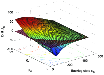
Figure 3: Drift backlog surface for $M=500$, $p_{r}=0.78$.

With (12) it is now possible to fully describe the stability of the CRDSA system for the case of having a user population $M$, a probability $p_{0}$ of fresh users generating new packets and a retransmission trial probability of $p_{r}$. Intuitively, the drift represents the tendency of the system to change over time and gives the direction of change of the backlog size. This means that for positive drifts the size of the backlog tends to increase by $d_{B}$ (i.e., more users experience lost packets and get backlogged). For negative drifts, the length of backlog decreases, which means that backlogged users successfully retransmit and get fresh again. A drift of 0 corresponds to an equilibrium point, which may be locally stable or instable. Fig. 3 shows the dynamics of the channel with the drift-backlog surface for the scenario $M=500$, $p_{r}=0.78$ and for varying $p_{0}$. The surface can be classified into three different areas: In the first area for $0\leq p_{0}\leq 0.01$ the drift-backlog-surface does not intersect the zero-drift plane and gets the tangent plane for $p_{0}=0.01$. In the second area for $0.01<p_{0}\leq 0.11$ the drift-backlog-surface intersects the zero-drift plane in three equilibrium points. In the third area for $0.11<p_{0}\leq 1$ the drift-backlog-surface intersects the zero-drift plane in a single equilibrium point which is located at the saturation point where all or almost all $M$ users are backlogged.

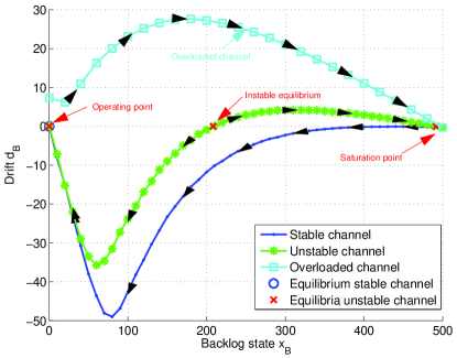
Figure 4: Backlog drift for a stable channel with $M=500$, $p_{r}=0.78$ and $p_{0}=0.01$, an instable channel with $M=500$, $p_{r}=0.78$ and $p_{0}=0.04$ and an overloaded channel with $M=500$, $p_{r}=0.78$ and $p_{0}=0.12$.

Fig. 4 shows the backlog drift of the three areas for three representative values of $p_{0}$, i.e. the intersection of the drift-backlog surface from Fig. 3 with the planes $p_{0}=\left\{0.01,0.04,0.12\right\}$.

As can be seen here, the drift for the stable configuration ($p_{0}\leq 0.01$) is always negative independent of the backlog state $x_{B}$ and approaches asymptotically a drift $d_{B}=0$, which means that the system always shows the tendency to lower the current backlog state until reaching the initial state. There is thus only one equilibrium point (globally stable) close to the initial state.

For the instable configuration ($0.01<p_{0}=0.04\leq 0.11$) it can be seen that after the initial equilibrium point (locally stable) and the following area of negative drift (up to $x_{B}\approx 209$) a second, locally instable equilibrium point is reached at $x_{B}=209$. When reaching this point the system can either fall back into the negative drift region for $x_{B}<209$ or enter the region of positive drift $x_{B}>209$. In the latter case the positive drift means that any movement to a higher backlog state (which is a consequence of the positive drift) results in an accelerated increase in number of backlogged users. This behavior then persists until reaching the third and final equilibrium point (locally stable) at $x_{B}\approx 500=M$. In this third equilibrium point now all or almost all $M$ users are backlogged and the system has reached the point of maximum load and minimum throughput. In case some of the users get unbacklogged, the drift is anyway positive and drives the channel back into the saturation. While there is a low probability that the channel returns in the high throughput region, the probability is fairly small and it can be expected that a very long time passes before this happens. For the overloaded configuration $0.11\leq p_{0}=0.12\leq 1.0$ the drift-backlog surface intersects the zero drift plane only once at the saturation point where all or almost all $M$ users are backlogged. Since there are no equilibria before and the drift is always positive, it can be expected that the system moves straight towards the saturation point after being started. An instable system may remain for some time in the desirable high throughput region of the operating point before getting instable and entering the low throughput region around the saturation point. For an overloaded configuration the channel moves directly to the saturation point.

From this observation the conclusion can be drawn that for a given system configuration $\Omega=\{d,N_{s},I_{max}\}$ the maximum traffic generation probability $p_{0}$ for which the system is still always stable is the one resulting in a drift contour which intersects the straight line $d_{B}=0$ at most once (Fig. 4). The resulting single equilibrium point is then locally and globally stable. For all other cases the channel is instable (e.g., instable configuration with $p_{0}=0.04$ in Fig. 4), meaning that earlier or later the backlog will increase into the total saturation point. If the single equilibrium point coincides with the saturation point, the system is overloaded. While it is - mathematically speaking - also stable in this scenario (locally and globally stable equilibrium) it is in total saturation with very low throughput and high delay. Since an operating point in this region is not viable for a communication system, in the remainder of this paper stable refers only to having one equilibrium point in the high throughput region.

With this framework, it is now possible to predict the stability of a channel with a certain set of parameters or to derive a set of parameters for which the channel is guaranteed to be stable. In [4] the validity of this model was verified against simulations in different scenarios.

IV Average Delay

From the stability model defined in the previous section it can be observed that the stability of a system with fixed $p_{0}$ benefits from a reduction of the retransmission probability $p_{r}$. Or in other words a configuration which is instable can always be stabilized by decreasing $p_{r}$. This comes however at the cost of a higher delay since reducing $p_{r}$ means increasing the average time before attempting a retransmission. On the one hand a low average delay (i.e. requiring $p_{r}$ to be as high as possible) is important for achieving a good QoS perception for the user. On the other hand remaining stable is important for user satisfaction as well, since an instable system will be driven into total saturation with asymptotically zero throughput and infinite delay. For a stable configuration however it is beneficial to have a $p_{r}$ as small as possible. The retransmission probability $p_{r}$ is thus a design parameter which can be optimized to achieve a delay as low as possible while being selected high enough to ensure a stable system operation. For this reason it is important to derive an analytical framework that makes it possible to compute the expected delay for a given system configuration in order to find the optimum choice for the design parameter $p_{r}$, e.g., to minimize the delay while remaining stable, but also for optimizing the maximum allowable packet generation probability $p_{0}$ or the maximum allowable user population $M$ which is treated in section V. While the stability model derived in the previous sections provides the mathematical framework to derive the overall set of parameters for which the RA is stable, this section deals with the computation of the expected delay for any set of parameters.

The analysis of SA in [13] followed the fundamental principles of Markov theory and derives the expected delay $D_{b}$ via Little’s theorem. According to this well known theorem, the average number of packets in a queuing system in stable conditions is the product of the packet arrival rate and the average dwell time in the queue. Applied to the stability analysis, the expected dwell time in the queue corresponds to the transmission delay $D_{b}$ of every packet (i.e. the time the packet remains in the channel until it is successfully received). The average number of packets in the channel is given by the expected backlog length $\overline{N}$ since every backlogged user has one pending transmission. In equilibrium the traffic arrival rate is equal to the serving rate, or in other words the channel throughput $S_{0}$ is equal to the offered load $G_{0}$. Following this analogy, the expected delay in a random access channel computes with Little’s theorem to:

$$D_{b}=\frac{\overline{N}}{S_{out}}$$ (13)

whereas

$$S_{out}=\sum_{n=0}^{M}S_{out}(n,p_{0})\cdot P_{n}$$

and $P_{n}$ is the probability of being in state $n$. Similarly the expected backlog length $\overline{N}$ can be computed as:

$$\overline{N}=\sum_{n=1}^{N}n\cdot P_{n}.$$

As it has been shown in [13] by numerical simulations, the values for $S_{out}$ and $\overline{N}$ can be closely approximated by the equilibrium point throughput $S_{0}$ and backlog state $n_{0}$, i.e. $S_{out}\approx S_{0}$ and $\overline{N}\approx n_{0}$. With this and (13) the expected delay $D_{b}$ gets:

$$D_{b}=\frac{n_{0}}{S_{0}}.$$ (14)

In order to show that the approximations of $S_{out}$ and $\overline{N}$ claimed by Kleinrock for SA are also valid in the case of CRDSA, the theoretical expected $D_{b}$ and the measured delay $D_{b}^{sim}$ have been compared for a representative CRDSA configuration $\Psi=\{M,p_{0},p_{r},d,N_{s},I_{max}\}=\{200,0.9,\frac{1}{60},2,100,10\}$.

The channel is stable in this configuration with an equilibrium point at $n_{0}=149.06$ and an average throughput of $S_{0}=0.46$. With (14) the expected delay gets $D_{b}=324.04\,\text{slots}=3.2404\,\text{frames}$. The average delay obtained by simulations is $D_{b}^{sim}=328.64\,\text{slots}=3.2864\,\text{frames}$, which is fairly close to $D_{b}$ and thus confirms firstly that the approximation for $S_{out}=S_{0}$ and $\overline{N}=n_{0}$ are also valid in the case of CRDSA, and secondly that the presented framework is suitable to estimate the average delay for a given channel configuration $\Psi$.

V Stability Comparison of SA and CRDSA for Stable Channels

With the ability to compute the expected delay for a given configuration $\Psi$, the stability of CRDSA can now be compared to the stability of SA. The stability of SA was deeply investigated in [13]. The comparison of the two stabilities is of particular interest since CRDSA offers much higher throughput rates, also for higher offered traffic loads but the question arises whether this gain comes at the cost of lower stability, or not. For comparing the two RA schemes it needs to be ensured that the conditions are comparable. For the stability and performance of the RA schemes a tradeoff exists between the total user population $M$, probability of traffic generation $p_{0}$ for unbacklogged users (user activity) and retransmission probability $p_{r}$ for backlogged users. As it was explained earlier, the RA channel for a finite user population can always be stabilized by choosing a low enough retransmission probability $p_{r}$. The selection of $p_{r}$ on the other hand impacts the delay, as shown before, e.g., a lower value of $p_{r}$ will have a positive impact on the stability of the system but results in longer delays. For comparing the SA and CRDSA stability the following optimization criteria can be chosen now:

1. Minimize the average delay $D_{b}$ for fixed user population $M$ and fixed traffic generation probability $p_{0}$

2. Maximize the size of the user population $M$ for fixed $p_{0}$ and average delay $D_{b}$

3. Maximize the supported traffic generation probability $p_{0}$ for fixed $M$ and $D_{b}$

In the following analysis of these three criteria, CRDSA configurations are specified by the set $\Psi$ whereas the SA configurations are denoted by the set $\Xi=\{M,p_{0},p_{r}\}$. It should be noted that the traffic generation probability $p_{0}$ refers to the probability of generating a packet in a transmission frame for CRDSA whereas it refers to the probability of generating a packet in a time slot for SA. To ensure a fair comparison among the two, i.e., having the same overall traffic generation, $p_{0}$ for SA is chosen to (15) in the following.

$$p_{0}^{SA}=\frac{p_{0}^{CRDSA}}{N_{s}}$$ (15)

V-A Comparison of Achievable Delay $D_{b}$

The design parameter $p_{r}$ impacts the stability of the system as well as the resulting average delay. For a given user population $M$ and traffic generation probability $p_{0}$ this forms an optimization problem of selecting the optimum $p_{r}^{*}$ which is low enough to guarantee a stable operation of the channel, while it should be as high as possible at the same time to provide a low average delay. This optimization problem can be formulated for CRDSA in the following way:

$$p_{r}^{*}=\underset{p_{r}\in[0,\dots,1]}{\operatorname{argmin}}\,D_{b}(\Psi,p_{r}).$$ (16)

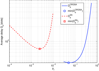
Figure 5: Comparison of minimum achievable delay for SA and CRDSA and $\Psi^{\prime}=\{M=400,p_{0}=0.263,p_{r},d=2,N_{S}=100,I_{max}=10\}$ and $\Xi^{\prime}=\{M=400,p_{0}=2.63\cdot 10^{-3},p_{r}\}$.

Fig. 5 illustrates this optimization problem. As it can be seen, the argument resulting in the minimum achievable delay for CRDSA and configuration $\Psi^{\prime}=\{M=400,p_{0}=0.263,p_{r},d=2,N_{s}=100,I_{max}=10\}$ gets:

$$p_{r,CRDSA}^{*}=\underset{p_{r}\in[0\dots 1]}{\operatorname{argmin}}\,D_{b}(\Psi^{\prime},p_{r})=5\cdot 10^{-2}$$

and the resulting minimum average delay computes to:

$$D_{b,\Psi^{\prime}}^{min}(p_{r}=p_{r,CRDSA}^{*}=5\cdot 10^{-2})=3.68\,\text{frames}\equiv 368\,\text{slots}.$$

For SA and comparable configuration $\Xi^{\prime}=\{M=400,p_{0}=2.63\cdot 10^{-3},p_{r}\}$ the optimization for the minimum achievable delay results in the optimum retransmission probability $p_{r,SA}^{*}=2.5\cdot 10^{-3}$ and an average delay of:

$$D_{b,\Xi}^{min}(p_{r}=p_{r,SA}^{*}=2.5\cdot 10^{-3})=707\,\text{slots}\equiv 7.07\,\text{frames}$$

While naturally the gain in terms of delay of the two different schemes changes with the other configuration parameters in $\Psi$ and $\Xi$, the results above show that in the given configuration CRDSA can save $48\%$ of the delay compared to SA in same conditions and guaranteeing a stable channel.

V-B Comparison of Supported User Population

The second optimization criterion is to determine the maximum user population $M$ which can be supported with the same average transmission delay $D_{b}$ while guaranteeing the stability of the channel. Finding the maximum user population $M^{*}$ for achieving an average delay $D_{b}^{0}$ forms an implicit optimization problem of $D_{b}(p_{r},M)$ with side condition (17):

$$g(p_{r},M)=D_{b}(p_{r},M)-D_{b}^{0}=0.$$ (17)

The solution of this optimization problem can be easily found with a Lagrange auxiliary function (18):

$$L(p_{r},M,\lambda)=D_{b}(p_{r},M)+\lambda[D_{b}(p_{r},M)-D_{b}^{0}].$$ (18)

The maximum supported user population $M^{*}$ for retransmission probability $p_{r}^{*}$ is then given simply by solving the set of equations:

$$\nabla L(p_{r},M,\lambda)=\left(\begin{array}[]{l}\frac{\partial L(p_{r},M,\lambda)}{\partial p_{r}}\\ \frac{\partial L(p_{r},M,\lambda)}{\partial M}\\ \frac{\partial L(p_{r},M,\lambda)}{\partial\lambda}\end{array}\right)=\underline{0}.$$

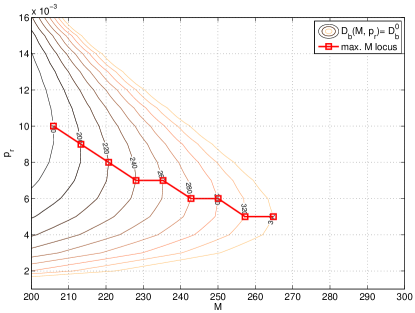
Figure 6: Locus for $D_{b}(M,p_{r})=D_{b}^{0}$ with $D_{b}^{0}\in[180\dots 340]\,\text{slots}$ for SA and locus of max. supported user population $M(D_{b}^{0})$.

resulting in the locus of tuples $(M^{*}(D_{b}^{0});p_{r}^{*}(D_{b}^{0}))$ shown in Fig. 6 for SA with $\Xi=\{M,2.63\cdot 10^{-3},p_{r}\}$ and for different values of $D_{b}^{0}$.

As it can be seen, the maximum user population, which can be supported at a maximum delay of $D_{b}^{0}=300\,\text{slots}$ gets $M^{*}_{SA}=250$ for an optimum $p_{r,SA}^{*}=6\cdot 10^{-3}$.

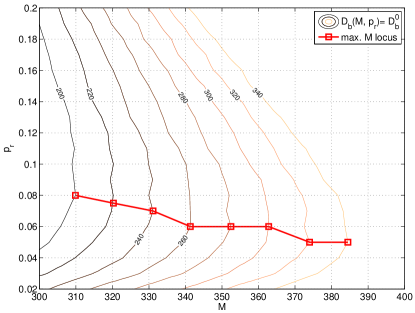
Figure 7: Locus for $D_{b}(M,p_{r})=D_{b}^{0}$ with $D_{b}^{0}\in[200\dots 340]\,\text{slots}$ for CRDSA and locus of max. supported user population $M(D_{b}^{0})$.

Fig. 7 shows the solution of the same optimization problem for CRDSA. The traffic generation probability was set to the equivalent value $p_{0}^{CRDSA}=2.63\cdot 10^{-1}$ in order to get the comparable traffic generation probability as in SA, resulting in the configuration $\Psi=\{M,2.63\cdot 10^{-1},p_{r},2,100,10\}$. As it can be seen here, the joint optimization results in $M^{*}_{CRDSA}=363$ for a retransmission probability $p_{r,CRDSA}^{*}=0.06$.

The comparison for this configuration shows that CRDSA can support 45% more users than SA while achieving the same average delay and being also guaranteed stable.

V-C Comparison of Supported Traffic Generation Probability

For the third optimization criterion, the user population is fixed together with the average delay to be achieved while guaranteeing at the same time that the channel remains stable. The optimization problem here is very similar to the previous one in section V-B and consists in finding the retransmission probability $p_{r}^{*}$ for which the the traffic generation probability $p_{0}^{*}$ is maximized for given user population $M$. Defining the Lagrange auxiliary function: (19)

$$L(p_{r},p_{0},\lambda)=D_{b}(p_{r},p_{0})+\lambda[D_{b}(p_{r},p_{0})-D_{b}^{0}]$$ (19)

and solving the set of equations given by:

$$\nabla\,L(p_{r},p_{0},\lambda)=\underline{0}$$

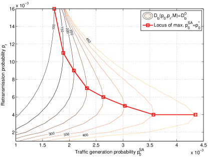
Figure 8: Joint optimization of $p_{0}$ and $p_{r}$ to achieve $D_{b}^{0}\,\text{slots}$ for SA with $\Xi=\{250,p_{0},p_{r}\}$.

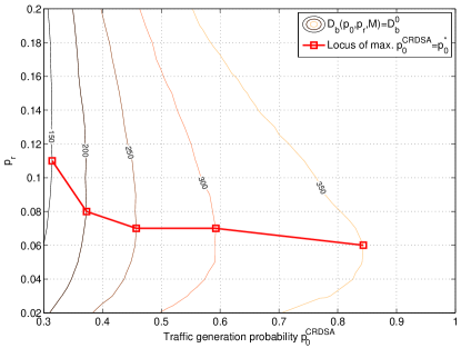
Figure 9: Locus for $D_{b}(p_{0},p_{r})=D_{b}^{0}$ with $D_{b}^{0}\in[150\dots 350]\,\text{slots}$ for CRDSA and locus of max. supported user population $M(D_{b}^{0})$.

provides the locus of optimum tuples $(p_{0}^{*},p_{r}^{*})$ shown in Fig. 8 for SA and in Fig. 9 for CRDSA and different $D_{b}^{0}$.

As it can be seen by comparing SA and CRDSA for e.g. $D_{b}^{0}=350\,\text{slots}$, the traffic generation probability supported by CRDSA is with $p_{0,CRDSA}^{*}=0.84$ a factor 2.8 higher than the one for SA with $p_{0,SA}^{*}=3\cdot 10^{-3}$. CRDSA thus allows users to generate traffic with a 2.8 times higher traffic generation probability than SA.

VI Average time before failure for CRDSA

The previous sections were focused on the investigation of stable channels. In many application scenarios instability may be acceptable if the time before getting instable is only sufficiently high. In stable channel conditions, the performance comparison of RA schemes could be done by comparing the minimum achievable delay $D_{b}$, the maximum number of supported users $M$ or the maximum traffic generation probability $p_{0}$. But for an instable channel configuration, these criteria do not apply anymore. In an instable channel the operating point will sooner or later reach the locally stable but undesired equilibrium point $n_{s}$ in the low throughput region, which can also coincide with the total saturation point, where all users are backlogged and the delay $D_{b}$ grows to infinity. Also the maximum user population $M$ or maximum traffic generation probability $p_{0}$ are no suitable measures. In an instable channel, $M$ and/or $p_{0}$ can grow arbitrarily while the channel will always remain instable. What changes is the time to reach $n_{s}$ which will be shorter with growing $M$ and $p_{0}$. With this in mind, the average time before the channel enters the instable region for the first time can be used as a suitable measure for comparing the behaviour of different RA schemes in instability.
Once the undesired operating point $n_{s}$ in the high load/low throughput area is entered, the channel may remain there potentially for a very long time (unless it is being reset). There is only a very small, but non-zero, probability to get out of this undesired operating point which depends on the configuration $\Psi$. As explained and shown in section III an instable system has three operating points, two of them locally stable and one locally instable. Among the two locally stable ones, one resides in the low load area (desired operating point) whereas the other one resides in the high-load/low throughput region (i.e. high number or all users backlogged). When in the locally instable operating point, the system has a chance to fall back into the desired region but the same chance to enter the undesired region, ending up in the low throughput operating point. In the SA analysis done by Kleinrock [13], this instable operating point is also denoted as the critical system state $n_{c}$. A measure for comparing the stability of different RA channels is then the average time before the critical state $n_{c}$ is reached for the first time, assuming further that the system will fall into the low throughput region, once $n_{c}$ is reached. In the Markov chain representation, the state $n_{c}+1=n_{u}$ is modeled as an absorbing state in order to simplify the analytical analysis. It should be noted that this is clearly only a model since in a real system the probability of leaving the high backlog state is non-zero, while it gets zero when using an absorbing state. In this work the focus is only to derive the time until the system is entering the instable state for the first time without looking at the time until it would leave the instability region again. The average first entry time $\overline{T}_{i}$ into state $i$ can be expressed recursively by

$$\overline{T}_{i}=1+\sum_{j=0}^{n_{c}}p_{ij}\cdot\overline{T}_{j}$$ (20)

whereas $p_{ij}$ denotes the state transition probability from state $i$ to state $j$

$$p_{ij} = Prob\left[N^{t+1}=j|N^{t}=i\right]=p_{x_{B},x_{B}^{\prime}}=$$ (21)

$$= \sum_{s,t}\binom{M-x_{B}}{\varphi}\cdot p_{0}^{\varphi}\cdot(1-p_{0})^{M-x_{B}-\varphi}\cdot$$

$$\binom{x_{B}}{\rho}\cdot p_{r}^{\,\rho}\cdot(1-p_{r})^{x_{B}-\rho}\cdot$$

$$q(\varphi+\rho,\varphi+x_{B}-x^{\prime}_{B})$$

For the computation of the First Entry Times (FET), it is now of interest to know the average time until reaching the critical state $n_{c}$ for the first time when starting from the initial state $x_{b}^{0}=0$, i.e., $\overline{T}_{0}^{n_{c}}$. The recursive formulation in (20) yields a set of linear equations:

$$\left[\begin{array}[]{c}\overline{T}_{0}\\ \overline{T}_{1}\\ \vdots\\ \overline{T}_{n_{c}}\\ \end{array}\right]=\left[\begin{array}[]{c}1\\ 1\\ \vdots\\ 1\\ \end{array}\right]+\left[\begin{array}[]{cccc}p_{00}&p_{01}&\ldots&p_{0{n_{c}}}\\ p_{10}&&&\\ \vdots&&&\\ p_{{n_{c}}0}&&&p_{{n_{c}}{n_{c}}}\\ \end{array}\right]\cdot\left[\begin{array}[]{c}\overline{T}_{0}\\ \overline{T}_{1}\\ \vdots\\ \overline{T}_{n_{c}}\\ \end{array}\right]\\$$

which can be expressed in matrix vector notation by Eq. (22)

$$\mathbf{t}=\mathbf{e}+\mathbf{P}\cdot\mathbf{t}$$ (22)

whereas $\mathbf{e}$ is the unity vector. The vector of interest with all the FETs for every state $i$ gets then

$$\mathbf{t}=\left(\mathbf{I}-\mathbf{P}\right)^{-1}\cdot\mathbf{e}$$ (23)

with $\mathbf{I}$ being the identity matrix and $\mathbf{e}$ the unity vector. For the stability measure of the channel the entry of interest is the first entry in $\mathbf{t}$ which represents the time $\overline{T}_{0}^{n_{c}}$ to reach $n_{c}$ starting from the initial state $x_{B}=0$.

VI-A Validation of the Model

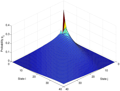
Figure 10: Markov state transition probabilities $p_{ij}$ for $\Psi_{0}$.

In order to illustrate the validity of the derived model, the markov state transition matrix and the FET is computed for a representative example here. The considered scenario is $\Psi_{0}=\{300,\,0.19,\,0.7,\,2,\,100,\,10\}$ which was chosen to result in an instable CRDSA channel with equilibrium points at $n_{0}=20$ (locally stable desired operating point), $n_{c}=40$ (locally instable equilibrium) and $n_{s}=247$ (locally stable undesired operating point). Since $n_{u}=n_{c}+1$ is an absorbing state it is sufficient to compute the Markov state transition probabilities in the range of states from $[0\dots n_{u}]$. Fig. 10 and 11 show the computed and simulated Markov state transition matrix $\mathbf{P}$ for $\Psi_{0}$.

As it can be seen from the two graphs, the transition probabilities resulting from the simulations match very well with the ones derived by numerical computation.
By solving the set of linear equations from (23), the computed FET time in this example results in $FET_{comp}=14.57\,\text{frames}$, where the average simulative FET reaches $FET_{sim}=13.59\,\text{frames}$, which is very close to the expected FET derived by computation.

VII FET comparison between CRDSA and SA

For a fair comparison between the FET of CRDSA and SA, configurations need to be selected which have the same initial conditions, i.e., the same user population $M$ and traffic generation probability $p_{0}$. The average delay $D_{b}$ cannot be used here since the average delay $D_{b}$ is infinite for an instable channel by definition as the channel will enter the saturation point with close to zero throughput.

A difficulty here consists in the fact that for an instable CRDSA configuration, the SA channel is getting overloaded.

On the other hand an instable SA configuration for which three equilibria exist results in a CRDSA configuration which is stable so no FET can be computed.

Fig. 12 shows the FET times for different configurations of CRDSA and SA for a user population of $M=500$.

As it can be seen, the FET for CRDSA and $p_{0}^{CRDSA}=10^{-1}$ is up to a factor 20 higher than for the equivalent SA configuration. It should be noted that SA is already in overload for a $p_{0}^{SA}=10^{-3}$. For this reason the SA FET curve does not show the time until reaching the critical state $n_{c}$ but the time until reaching the saturation point $n_{s}$ instead.

Fig. 12 furthermore shows the FET curve for CRDSA until reaching the saturation point $n_{s}$. The FETs for this curve are slightly higher than for $n_{c}$ as could be expected. This result also confirms the assumption to compute the FET times by modeling $n_{c}$ as an absorbing state instead of computing the full Markov chain up to $n_{s}$, since once $n_{c}$ is reached also $n_{s}$ is reached very fast. The SA curve in Fig. 12 could arise the impression that the FET curve is flat and has a qualitatively different shape than the CRDSA curve. This is actually not the case and the $\overline{T}_{0}^{n_{c}}$ for $p_{r}=0.5$ is indeed higher than for $p_{r}=0.9$ with a value of $\overline{T}_{0}^{n_{c}}(p_{r}=0.5)=6809.04\,\text{slots}$ and $\overline{T}_{0}^{n_{c}}(p_{r}=0.9)=6798.45\,\text{slots}$. In this configuration the SA channel is already so overloaded that also a large decrease of the retransmission probability $p_{r}$ does not have a significant impact anymore. Once the traffic generation probability $p_{0}^{SA}$ is lowered, the impact of $p_{r}$ gets more visible as it can be seen from the last curve in Fig. 12, which was computed for $p_{0}^{SA}=3.57\cdot 10^{-4}$. Also for this lower $p_{0}^{SA}$ the $\overline{T}_{0}^{n_{c}}$ is much lower than for CRDSA with a higher $p_{0}^{CRDSA}=10^{-1}$, showing that for an instable configuration CRDSA is remaining stable much longer than SA.

VIII Summary and Conclusions

In this paper, a theoretical model for the stability of CRDSA as representant for SIC RA schemes was developed. With this model it is possible to draw qualitative and quantitative conclusions about the stability of the communication channel. The presented framework enables the estimation of the average delays experienced in stable channel configurations. The stable CRDSA and SA RA channels were optimized for achieving a minimum delay, maximizing the user population while achieving a delay target or deriving the maximum traffic generation probability for a given user population and delay target for which the channel is stable. Numerical results were presented which allow a direct comparison of the performance of CRDSA and SA. These results have shown that CRDSA does not only provide a higher throughput and lower PLR than SA but is also capable to achieve lower delays and higher user population and traffic generation probabilities than SA while being stable. Finally the stability framework was extended towards instable channel configurations of CRDSA and makes possible to predict the average time before reaching instability. The derived model for CRDSA was validated against simulations and the stability behaviour of CRDSA was compared to the one of SA for instable channels. Also here CRDSA showed a much better performance by reaching way higher average times before failure than SA. Besides the analysis of the stability behaviour of a channel, the presented framework enables the computation of the optimum design parameters, in particular $p_{r}$ for which the channel either remains guaranteed stable while minimizing the average delay or the $p_{r}$ for an instable channel, which results in the desired FET time.

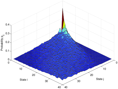
Figure 11: Simulated Markov state transition probabilities $p_{ij}$ for $\Psi_{0}$ (1000 runs).

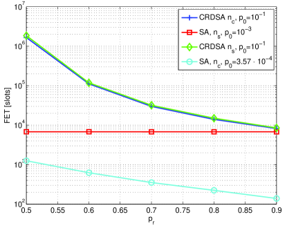
Figure 12: FET times for CRDSA and SA.

References

- [1] E. Casini, R. De Gaudenzi, and O. Herrero, “Contention resolution diversity slotted ALOHA (CRDSA): An enhanced random access scheme for satellite access packet networks,” Wireless Communications, IEEE Transactions on, vol. 6, no. 4, pp. 1408 –1419, April 2007.
- [2] G. Liva, “A slotted aloha scheme based on bipartite graph optimization,” in Source and Channel Coding (SCC), 2010 International ITG Conference on, Siegen, Germany, April 2010, pp. 1 –6.
- [3] E. Paolini, G. Liva, and M. Chiani, “High throughput random access via codes on graphs: Coded slotted aloha,” in Communications (ICC), 2011 IEEE International Conference on, Kyoto, Japan, June 2011, pp. 1 –6.
- [4] C. Kissling, “On the stability of contention resolution diversity slotted aloha (CRDSA),” in (GC), 2011 Global Communications Conference, Houston, TX, USA, December 2011, pp. 1–6.
- [5] D. Bertsekas and R. Gallager, Data Networks, 2nd ed. Prentice Hall.
- [6] L. Kleinrock and S. S. Lam, “Packet-switching in a slotted satellite channel,” in Proceedings of the June 4-8, 1973, national computer conference and exposition, ser. AFIPS ’73. New York, NY, USA: ACM, 1973, pp. 703–710.
- [7] R. M. Metcalfe and D. R. Boggs, “Ethernet: distributed packet switching for local computer networks,” Commun. ACM, vol. 19, pp. 395–404, July 1976.
- [8] J. Capetanakis, “Tree algorithms for packet broadcast channels,” Information Theory, IEEE Transactions on, vol. 25, no. 5, pp. 505 – 515, September 1979.
- [9] S. S. Lam, “Packet switching in a multi-access broadcast channel with application to satellite communication in a computer network,” S.S. Lam, Department of Computer Science, University of California, Los Angeles, March 1974, also in Tech. Rep. UCLA-ENG-7429, April 1974.
- [10] O. del Rio Herrero and R. D. Gaudenzi, “A high-performance MAC protocol for consumer broadband satellite systems,” IET Conference Publications, vol. 2009, no. CP552, pp. 512–512, 2009.
- [11] G. Choudhury and S. Rappaport, “Diversity aloha–a random access scheme for satellite communications,” Communications, IEEE Transactions on, vol. 31, no. 3, pp. 450 – 457, March 1983.
- [12] N. Abramson, “The throughput of packet broadcasting channels,” Communications, IEEE Transactions on, vol. 25, no. 1, pp. 117 – 128, January 1977.
- [13] L. Kleinrock and S. Lam, “Packet switching in a multiaccess broadcast channel: Performance evaluation,” Communications, IEEE Transactions on, vol. 23, no. 4, pp. 410 – 423, April 1975.
- [14] G. Liva, “Graph-based analysis and optimization of contention resolution diversity slotted aloha,” Communications, IEEE Transactions on, vol. 59, no. 2, pp. 477–487, February 2011.
- [15] R. G. Gallager, “Low-density parity-check codes,” MA: M.I.T. Press, 1963.
- [16] N. Abramson, “The aloha system: Another alternative for computer communications,” in Proceedings of the 1970 Fall Joint Comput. Conf., AFIPS Conf., vol. 37, Montvale, N. J., 1970, pp. 281–285.
- [17] L. G. Roberts, “Aloha packet system with and without slots and capture,” SIGCOMM Comput. Commun. Rev., vol. 5, pp. 28–42, April 1975.
- [18] R. Gallager, “A perspective on multiaccess channels,” Information Theory, IEEE Transactions on, vol. 31, no. 2, pp. 124 – 142, March 1985.
- [19] R. Murali and B. Hughes, “Random access with large propagation delay,” Networking, IEEE/ACM Transactions on, vol. 5, no. 6, pp. 924 –935, December 1997.
- [20] A. Carleial and M. Hellman, “Bistable behavior of aloha-type systems,” Communications, IEEE Transactions on, vol. 23, no. 4, pp. 401 – 410, April 1975.