TRIGGERED STAR FORMATION SURROUNDING WOLF-RAYET STAR HD 211853

Abstract

The environment surrounding Wolf-Rayet (W-R) star HD 211853 is studied in molecular, infrared, as well as radio, and Hi emission. The molecular ring consists of well-separated cores, which have a volume density of 10³ cm^-3 and kinematic temperature $\sim$20 K. Most of the cores are under gravitational collapse due to external pressure from the surrounding ionized gas. From the spectral energy distribution modeling toward the young stellar objects, the sequential star formation is revealed on a large scale in space spreading from the W-R star to the molecular ring. A small-scale sequential star formation is revealed toward core ”A”, which harbors a very young star cluster. Triggered star formations are thus suggested. The presence of the photodissociation region, the fragmentation of the molecular ring, the collapse of the cores, and the large-scale sequential star formation indicate that the collect and collapse process functions in this region. The star-forming activities in core ”A” seem to be affected by the radiation-driven implosion process.

1 Introduction

The feedback of massive stars is expected to strongly influence their surrounding interstellarmedium (ISM) through stellar radiation, energetic wind, and the ejection of the elemental composition. The shock front (SF) that emerges as bubbles around massive stars expand can compress the ISM and trigger star formation in very dense layers (Chen et al. 2007).

Two models have been proposed to explain the effect of massive stars on star formation: collect and collapse (Elmegreen & Lada 1977) and radiation-driven implosion (RDI; Lefloch & Lazareff 1994; Ogura 2010). The former takes place in a larger spatial size ($\sim$10 pc) with a longer timescale (a few Myr), whereas the latter takes place in a smaller spatial size ($\sim$1 pc) with a shorter timescale (0.5 Myr; Ogura 2010). In the ”collect and collapse” scenario, the ionization front (IF) generated from the Hii region gathers molecular gases and collects a dense shell between the IF and the SF. The gas and dust in the collected layer collapse to form stars when they reach the critical density (Chen et al. 2007; Ogura 2010). This process can selfpropagate and lead to sequential star formation (Elmegreen & Lada 1977). Star formation induced through the ”collect and collapse” process has been revealed in the borders of several Hii regions (Deharveng et al. 2003, 2005, 2008; Zavagno et al. 2006, 2007; Pomar‘es et al. 2009; Petriella et al. 2010;Brand et al. 2011). The so-called RDI process has been proposed to account for the evolution of bright-rimmed clouds whose surfaces are ionized by the UV photons from massive stars and trigger the star formation therein (Bertoldi 1989; Bertoldi & McKee 1990; Hester & Desch 2005; Miao et al. 2009; Gritschneder et al. 2009; Bisbas et al. 2011; Haworth & Harries. 2012). The IFs generate a shock that compresses into the cloud and causes the dense clumps to collapse (Chen et al. 2007). Candidates for star formation by RDI have been found in many bright rimmed clouds associated with IRAS point sources (Sugitani et al. 1991; Sugitani & Ogura 1994; Urquhart et al. 2004, 2006, 2007; Morgan et al. 2010).

The Wolf.Rayet (W-R) stars, initially more massive than $\sim$40M_☉, have typical mass-loss rates of 10^-5 M_☉ yr^-1 and strong stellar winds faster than 1000 km s^-1. They can blow stellar wind bubbles with radii of $\sim$10 to $\sim$100 pc and expanding velocities of several km s^-1 (Marston 1996;Martín-Pintado et al. 1999). The expanding bubbles can push away the molecular gas and create molecular layers that fragment into condensations well separated in due time. The ”collect and collapse” process is expected to happen in the shells swept up by such expanding stellar wind bubbles (Whitworth et al. 1994). However, the samples of triggered star formation surrounding W-R stars are rare and few previous works have focused on star-forming activities in such regions. In this paper, we provide a sample region where triggered star formation is witnessed.

HD 211853 is located at the center of an optically bright region named shell B in the Hii region Sh2-132 (Sharpless 1959; Harten et al. 1978). The Hii region linked to shell B is excited by a massive O-type star BD+55.2722 and the W-R starHD211853 (Vasquez et al. 2010). While it is the main ionizing source of the ring nebula (Cappa et al. 2008), the W-R star HD 211853 (WR 153ab) is a binary system. The spectral types of the two W-R components are WN6 and WCE+06 (Nishimaki et al. 2008). The velocity of its stellar wind is as high as 1500.1800 km s.1, leading to a high mass-loss rate of 10^-4.5 M_☉ yr^-1 (Nishimaki et al. 2008). A ring nebula associated with HD 211853 is easily identified in radio emission, in polycyclic aromatic hydrocarbon (PAH) emission, and in molecular emission (Vasquez et al. 2010; Cappa et al. 2008). Figure 1 presents a composite color image of this region. Blue corresponds to the DSS-R optical emission, green to the radio emission detected in the Canadian Galactic Plane Survey (CGPS; Taylor et al. 2003) at 1420 MHz, and red to 8.3 $\micron$ emission detected at the Midcourse Space Experiment (MSX) A band.

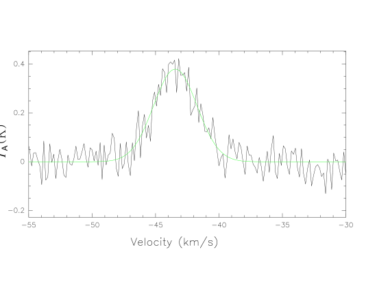
Figure 2: Spectrum of ¹²CO (1-0) at the position of the Wolf-Rayet star HD 211853 averaged over 1$\arcmin$. The green solid line is the Gaussian fit curve.

It can be seen that the radio emission is embraced by the 8.3 $\micron$ emission, which forms a ring-like structure. A photodissociated region (PDR) has been identified, and possible triggered star formation in this region is suggested (Vasquez et al. 2010). As shown in Figure 2 of Saurin et al. (2010), three star clusters, ”Teutsch 127,” ”SBB 1,” and ”SBB 2,” have been found in this region; the hierarchical structure and age distribution of the star clusters show evidence of triggered star formation (Saurin et al. 2010). However, studies of the star-forming activities in this region are far from mature. In this paper, through detailed analysis of molecular emission and characteristics of young stellar objects (YSOs), we have revealed the picture of triggered star formation in this region.

2 Observations and Database

The observations of ¹²CO (1-0), ¹³CO (1-0), and C¹⁸O (1-0) were carried out with the Purple Mountain Observatory (PMO) 13.7 m radio telescope in 2011 January. The new 9-beam array receiver system in single-sideband (SSB) mode was used at the front end. The array pixels are sideband separation SIS mixers yielding 18 independent IF outputs. The properties of the Solid-State Imaging Spectrometer (SIS) mixers are introduced in Shan et al. (2009). ¹²CO (1-0) was observed at the upper sideband, while ¹³CO (1-0) and C¹⁸O (1-0) were observed simultaneously at the lower sideband. FFTS spectrometers were used as back ends, which have a total bandwidth of 1 GHz and 16384 channels, corresponding to a velocity resolution of 0.16 km s^-1 for ¹²CO (1-0) and 0.17 km s^-1 for ¹³CO (1-0) and C¹⁸O (1-0). The half-power beam width was 56$\arcsec$, and the main beam efficiency was $\sim 0.5$ during our observation period. The pointing accuracy of the telescope was better than 4$\arcsec$. The typical system temperature (T_sys) in SSB mode was around 110 K and varied about 10% for each beam. The On-The-Fly (OTF) observing mode was applied. The antenna continuously scanned a region of 22$\arcmin\times 22\arcmin$ centered on the Wolf-Rayet star HD 211853 with a scan speed of 20$\arcsec$ s^-1. The OTF data were then converted to three-dimensional cube data with a grid spacing of 30$\arcsec$. Because the edges of the OTF maps are very noisy, only the central 14$\arcmin\times 14\arcmin$ region was selected to be analyzed. The typical rms noise level was 0.2 K in T${}_{A}^{*}$ for ¹²CO (1-0), and 0.1 K for ¹³CO (1-0) and C¹⁸O (1-0). For the data analysis, the GILDAS software package including CLASS and GREG was employed (Guilloteau & Lucas, 2000).

Neutral hydrogen (HI) 21 cm line data were from CGPS with intensities shown as brightness temperature T_mb. The synthesized beam and rms bright temperature in a 0.82 km s^-1 channel were $\sim 1\arcmin$ and 3 K, respectively. Radio continuum data and images at 1420 MHz were extracted from the CGPS (Taylor et al., 2003) and the NRAO Very Large Array (VLA) Sky Survey (NVSS, Condon et al. (1998)). The positions and fluxes of the NVSS sources were obtained from the NVSS catalog (Condon et al., 1998). The CGPS 1420 MHz data had a synthesized beam of $\sim 50\arcsec$ and a noise level of $\sim 3$ mJy beam^-1. The NVSS image had a spatial resolution of 45$\arcsec$ and an rms brightness fluctuation of $\sim 0.45$ mJy beam^-1 (Stoke I). MSX A-band data were extracted from the MSX Galactic Plane Survey (Price et al., 2001), which has a spatial resolution of $\sim 18\arcsec.3$. Spitzer IRAC data and Two Micron All Sky Survey (2MASS) data were obtained from Qiu et al. (2008), both of which have good spatial resolutions of $\sim 2\arcsec$. We also obtained SCUBA 450 $\micron$ and 850 $\micron$ continuum data from the SCUBA Legacy Catalogues (Di Francesco et al., 2008). At 850 and 450 $\micron$, the resolutions of SCUBA data are of $\sim 14\arcsec$ and $\sim 9\arcsec$, respectively.

3 Results

3.1 Molecular emission

The ¹²CO (1-0), ¹³CO (1-0), and C¹⁸O (1-0) emissions were observed simultaneously. However we did not detect any C¹⁸O (1-0) emission in this region above 3$\sigma$ (0.3 K), which indicates low column density in this region. ¹²CO (1-0) emission was detected in almost the whole region even at the position of the Wolf-Rayet star HD 211853. ¹³CO (1-0) emission was only detected in the ring-like region, but not within it. The detailed analysis of the molecular emission is described below.

3.1.1 The systemic velocity of the molecular clumps

In Figure 2, we present the 1$\arcmin$ averaged spectrum of ¹²CO (1-0) at the position of the Wolf-Rayet star. ¹²CO (1-0) emission is significantly detected. From the gaussian fit, the peak antenna temperature is 0.38$\pm$0.02 K, about 8$\sigma$ level (1$\sigma$ equal to 0.05 K estimated from the baseline). It has a line width of 4.1$\pm$0.2 km s^-1 and a peak velocity of -43.4$\pm$0.01 km s^-1.

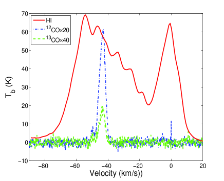
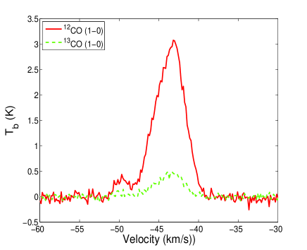
Figure 3: Left: Spectra of ¹²CO (1-0), ¹³CO (1-0) and HI averaged over an area of 14$\arcmin\times 14\arcmin$ centered at the Wolf-Rayet star HD 211853. Right: Zoomed in averaged spectra of ¹²CO (1-0), and ¹³CO (1-0).

The left panel of Figure 3 presents the 14$\arcmin\times 14\arcmin$ averaged spectra of the HI 21 cm line, line ¹²CO (1-0) and line ¹³CO (1-0). The right panel of Figure 3 shows the zoomed in averaged spectra of the ¹²CO (1-0) and ¹³CO (1-0) lines. There are two components in the ¹²CO (1-0) and ¹³CO (1-0) emission, which was also noticed by Vasquez et al. (2010). The narrow one peaks at -50 km s^-1, while the other broader one ranges from -48 km s^-1 to -39 km s^-1.

Are both components related to this region? We argue that the -50 km s^-1 maybe a foreground cold cloud, rather than part of this region based on the following two aspects.

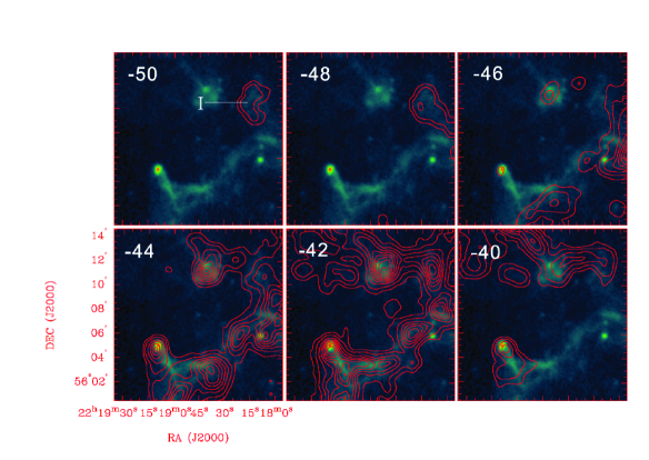
Figure 5: Channel maps of ¹²CO (1-0). The middle velocities are plotted on the upper-right corners of each panel. The integrated velocity interval in each panel is 2 km s^-1. The contours are from 20% to 90% of the peak intensity (4.6 K$\cdot$km s^-1). The background image shows the 8.3 $\micron$ emission detected at the MSX A band. The position of core ”I” is marked in the -50 km s^-1 panel.

(1). The integrated emission of ¹²CO (1-0) in the first two panels of Figure 5 is concentrated in an isolated and compact core (denoted as core ”I”) north-west of HD 211853. We did not detect this component in the other positions. Additionally, from the P-V diagrams in Figure 6, one can see that the -50 km s^-1 component is also not connected to the other component in velocity space. Vasquez et al. (2010) argued that the ¹²CO (1-0) emission between -53.4 and -46.0 km s^-1 is also associated with the ring nebula. However, their conclusion may be misleading because their integrated map is contaminated by the emission between -48 to -46 km s^-1. As the channel map shows, the emission in their clouds E and F is dominated by the emission between -48 and -39 km s^-1, rather than the -50 km s^-1 component.

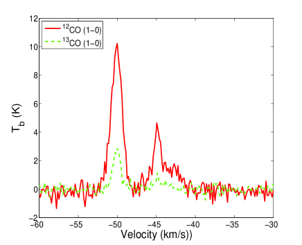
Figure 4: Left: Spectra of ¹²CO (1-0), ¹³CO (1-0) and HI taken from the emission peak of the component at -50 km/s (core ”I”). Right: Zoomed in spectra of ¹²CO (1-0), and ¹³CO (1-0) at core ”I”.

(2). The left panel of Figure 4 presents the spectra of the HI 21 cm line, ¹²CO (1-0) and ¹³CO (1-0) lines at the peak of core ”I”. The right panel of Figure 4 shows the zoomed in spectra of the ¹²CO (1-0) and ¹³CO (1-0) lines. One can see that the HI emission at the peak of core ”I” has a very narrow absorption dip. Together with the narrow line width of the molecular emission, an HI Narrow Self-Absorption (HINSA) system can be identified, suggesting that core ”I” is more likely a foreground cold cloud (Li & Goldsmith, 2003). As shown in Table 2, the kinematic temperature of core ”I” (14.6$\pm$0.3 K) is much lower than that of core ”F” (21.7$\pm$1.0 K), indicating that core ”I” is more quiescent than core ”F”.

In conclusion, the -50 km s^-1 molecular component is more likely from a foreground cold cloud, rather than a part of the molecular environment surrounding HD 211853. However because the -50 km s^-1 molecular component is very near the ring nebular in the spatial and velocity space, it may also interact with the expanding molecular ring, which needs further observations to confirm.

From the Gaussian fit, the averaged ¹³CO (1-0) spectrum peaks at -43.6$\pm$0.1 km s^-1, very similar to that of the ¹²CO (1-0) emission taken from the central Wolf-Rayet star (-43.4$\pm$0.01 km s^-1). Thus, we adopt -43.5 km s^-1 as the overall systemic velocity of the molecular emissions in this region.

3.1.2 The properties of molecular cores

Figure 5 displays the channel maps of ¹²CO (1-0) emission in contours overlaid on the 8.3 $\micron$ emission in the MSX A band. The middle velocities of each panel are plotted on the upper-right corners. In each panel, the integrated velocity interval is 2 km s^-1. The contours are from 20% to 90% of the peak intensity in each panel. It can be seen that the ¹²CO (1-0) emission is very clumpy. The blue shifted gas (-46 km s^-1 panel) distributes in the western and southern regions, while the red shifted gas (-40 km s^-1 panel) is mainly in the northern and eastern regions, indicating a velocity gradient from north-east to south-west. The gas at -42 and -44 km s^-1 forms a ring-like structure harboring several well separated cores. The ring-like molecular structure perfectly coincides with the 8.3 $\micron$ emission in the MSX A band.

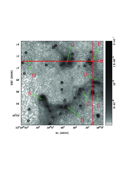
Figure 7: ¹³CO (1-0) integrated intensity map overlayed on MSX A band emission. The contours are from 10% to 90% of the peak (7.8 K$\cdot$ km s^-1). ”Triangles” represent MSX point sources, ”boxes” IRAS point sources, and ”stars” AKARI point sources. The Wolf-Rayet star is drawn as ”cross”. The molecular cores are denoted from ”A” to ”H”. The horizon and vertical dashed lines represent the directions of the P-V cuts in Figure 6.

Figure 6 presents the P-V cuts along two orientations denoted by the red dashed lines in Figure 7. From the P-V diagrams, it is clear that the -50 km s^-1 component is separated with the -43.5 km s^-1 component. An amazing aspect of the P-V cuts is that the relative velocity of the gas increases with the distance to the WR star from near to far, following a ”Hubble law” like distribution, as denoted by the dashed lines.

Figure 7 displays the integrated intensity map of ¹³CO (1-0) overlaid on the 8.3 $\micron$ emission in gray scale, which is integrated from -48 to -39 km s^-1. The contours are from 10% ($\sim 8\sigma$) to 90% of the peak emission. Eight cores are identified and denoted from ”A” to ”H”. The Wolf-Rayet star HD 211853 is drawn as a ”cross”. IRAS, MSX and AKARI point sources are marked with ”boxes”, ”triangles,” and ”stars”, respectively. However, one should keep in mind that many of these point sources may be not real; rather, they may correspond to some variations of brightness in the infrared emission along the filamentary structures. More observations are needed to constrain their properties. For convenience, we still call them ”point sources” in the following text. These cores form a ring-like structure surrounding HD 211853, and they are associated with the 8.3 $\micron$ emission in the MSX A band. Most of the infrared point sources are distributed in the molecular ring. Core ”A” is associated with an IRAS source ”IRAS 22172+5549”, while the emission peaks of the other cores seem to be separated from the infrared point sources, which will be discussed later in Section 4.3.

Taking into account the effect of beam smearing, the radii of the cores are calculated as R=$\frac{\sqrt{4A/\pi-\theta_{b}^{2}}}{2}$, where A is the projected area of each core and $\theta_{b}$ is the beam width. Adopting a distance of 3 kpc (Cappa et al., 2008), the radii of the cores are calculated and listed in the fourth column of Table 1. The average radius is 1 pc.

Figure 8 presents the spectra of ¹²CO (1-0), ¹³CO (1-0), and C¹⁸O (1-0) at the emission peaks of the cores. The spectra at core ”E” are totally blue shifted, while at core ”H” the spectra are red-shifted. The peak velocities of the other cores coincide with or slightly deviate from the systemic velocity. The results of the Gaussian fit to these spectra are listed in Table 1. Core ”G” has the largest line width and antenna temperatures, while core ”H” has the smallest ones. The line width of ¹³CO (1-0) ranges from 1.3 to 2.6 km s^-1 with a mean value of 2.1 km s^-1.

Assuming ¹²CO (1-0) emission is optically thick and ¹³CO (1-0) is optically thin, we derived the parameters of the cores including the excited temperatures T_ex, column densities of H₂, N${}_{H_{2}}$, and optical depth of ¹³CO (1-0) lines under the local thermal equilibrium (LTE) assumption following Garden et al. (1991). Typical abundance ratios [H₂]/[¹²CO]=$10^{4}$ and [¹²CO]/[¹³CO]=60 were used in the calculations (Deharveng et al., 2008). The volume density of H₂ is calculated as n${}_{H_{2}}$=N${}_{H_{2}}$/2R. Then the core mass can be derived as M=$\frac{4}{3}\pi\cdot R^{3}\cdot n_{H_{2}}\cdot m_{H_{2}}\cdot\mu_{g}$, where $m_{H_{2}}$ is the mass of a hydrogen molecule and $\mu_{g}$=1.36 is the mean atomic weight of the gas. The derived parameters are listed from Columns 3-7 in Table 2. The N${}_{H_{2}}$ ranges from $1.8\times 10^{21}$ to $1.4\times 10^{22}$ cm^-2. The optical depth of ¹³CO (1-0) is around 0.3. The core masses range from 21 M_☉ (”H”) to 1061 M_☉ (”G”) with a mean value of 400 M_☉.

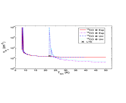
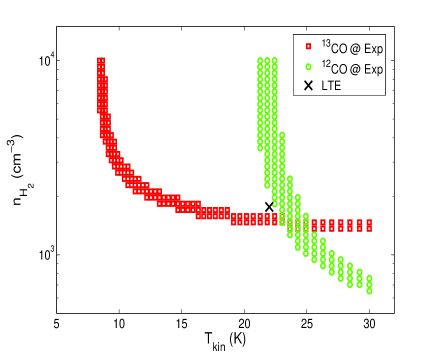
Figure 9: Non-LTE model fitting of ¹²CO (1-0) and ¹³CO (1-0) at the emission peak of core ”A”. Left: parameters run through T_kin of [5,50] K and n${}_{H_{2}}$ of [10²,10⁶] cm^-3 in log space. Right: parameters run through T_kin of [8,30] K and n${}_{H_{2}}$ of [2.5$\times$10²,10⁴] cm^-3 in log space.

We also applied RADEX (Van der Tak et al., 2007), a one-dimensional non-LTE radiative transfer code, which uses the escape probability formulation assuming an isothermal and homogeneous medium without large-scale velocity fields, to constrain the physical conditions, such as density and kinetic temperature, of the cores. In the first running, we explored a range of H₂ volume densities and temperatures of [10²,10⁶] cm^-3 and [5,50] K. The molecular column densities, which are also input parameters required, are fixed according to the H₂ volume densities as N(X)=n${}_{H_{2}}\cdot$2R$\cdot$X(x), where X(x) is the relative abundance ratio of the molecule. For ¹²CO (1-0), X(x)=10^-4, and for ¹³CO (1-0), X(x) is adopted as 1.67$\times 10^{-6}$. The model parameters were selected to satisfy $\mid T_{mod}-T_{obs}\mid\leq 3\sigma$, where $T_{mod}$ and $T_{obs}$ are the modeled and observed brightness temperature of the molecule transition, respectively. As shown in the left panel of Figure 9, the kinematic temperatures and H₂ volume densities can be well constrained by modeling both the ¹²CO (1-0) and ¹³CO (1-0) lines. Two geometries, static spherical and expanding spherical (similar to large velocity gradient (LVG) approximation), were chosen in this running. It can be seen that both geometry assumptions give nearly the same results for ¹³CO (1-0) lines, while for ¹²CO (1-0) lines, static spherical models give slightly higher volume densities than expanding spherical at higher kinematic temperatures. However, in the overlapping region, the deviations of the two geometries are small enough to be ignored. We narrowed the parameter space in the second running assuming the expanding spherical geometry. The range H₂ volume densities and temperatures in the second running are [2.5$\times$10²,10⁴] cm^-3 and [8,30] K, respectively. As shown in the right panel of Figure 9, the kinematic temperatures and volume densities of H₂ can be well constrained in the overlapping region of ¹²CO (1-0) and ¹³CO (1-0) tracks. The best physical parameters from RADEX are obtained by averaging the parameters in the overlapping region and are displayed from Columns 7-14 in Table 2.

It is interesting to note that the excitation temperatures of ¹²CO (1-0) obtained from RADEX are perfectly consistent with those calculated under LTE assumption. The excitation temperatures of ¹³CO (1-0) are much lower than those of ¹²CO (1-0). The optical depths of ¹³CO (1-0) obtained from RADEX are larger than those obtained from LTE conditions. The kinematic temperatures are always larger than the excitation temperatures of ¹²CO (1-0). The volume densities of H₂ and core masses calculated in RADEX roughly agree with those from LTE calculations.

3.2 Radio continuum emission, HI emission and PAH emission

From the radio emission detected in CGPS at 1420 GHz, Vasquez et al. (2010) obtained an rms n_e=20 cm^-3 and M_HII=1500 M_☉ in this region. As shown in the upper panels of Figure 10, nine NVSS radio sources (shown in blue dashed contours) are located in this region, and most of them are bordered by the 8.3 $\micron$ emission ring shown in red solid contours. The nine radio sources are not individual HII regions, but are instead high brightness components of the large HII region. They reflect the fluctuation and non-uniformity of the ionized gas distribution within the large HII region. The Wolf-Rayet star is associated with NVSS source ”1”, and the molecular core ”A” is associated with NVSS source ”5”. Following Panagia & Walmsley (1978), the electron densities, emission measures and masses of ionized hydrogen of these NVSS sources are derived by assuming an electronic temperature of 8000 K. However, those parameters listed in Table 3 can only be treated as lower limits due to the missing flux of VLA. NVSS ”4”, ”5” and ”2” in the yellow dashed box show very high electronic densities and form an ionization front interacting with the molecular ring. NVSS ”1” and ”3” seem to interact with the northern part of the molecular ring, mainly with core ”G”.

We integrated HI emission from -48 km s^-1 to -39 km s^-1 and displayed the integrated intensity map in gray scale in the upper panel of Figure 10. The HI emission is very diffuse with an integrated intensity gradient in the N-S orientation. The HI emission also has a shell-like appearance in the southern part, which is associated with the 8.3 $\micron$ emission. An HI cavity is found within the yellow dashed box, where the ionization front exists. Assuming that the HI 21 cm line is optically thin and spin temperature $T_{s}\gg h\nu/k$, the average column density of HI can be calculated as $N_{HI}=1.82\times 10^{18}\times\int\overline{T_{b}}dv$ (cm^-2). Based on the averaged spectrum of HI shown in the left panel of Figure 3, the average column density of HI in the whole region of shell B is about $9.4\times 10^{20}$ cm^-2. The total mass of HI is estimated to be 1100 M_☉, which is comparable to the total mass of HII ($\sim$1500 M_☉) (Vasquez et al., 2010).

The ring-like feature of the 8.3 $\micron$ emission in MSX A band was been revealed by Cappa et al. (2008); Vasquez et al. (2010). It clearly shown as red contours in the upper-panel of Figure 10 in this paper. The 8.3 $\micron$ emission is dominated by PAH emission and indicates the presence of PDRs (Vasquez et al., 2010). IRAC 8 $\micron$ emission shown in color scale in the lower panel of Fig.10 also reveals a shell-like structure of PAH emission.

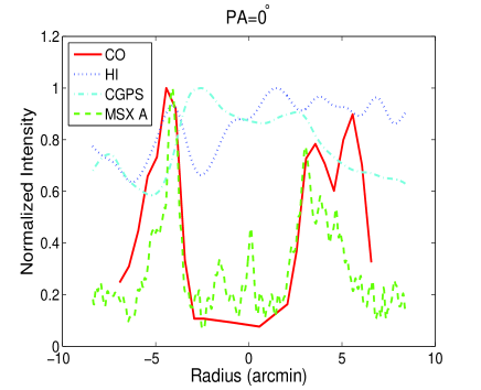
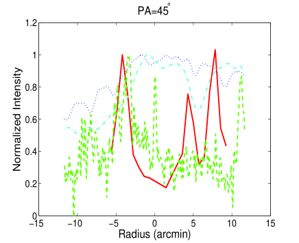
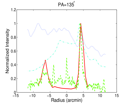
Figure 11: Normalized intensity distributions of CO, HI, 1420 MHz radio emission detected in CGPS and 8.3 $\micron$ emission detected in the MSX A band along four orientations centered on the Wolf-Rayet star.

In Figure 11, we analyze the distribution of the normalized intensities of ¹²CO (1-0) emission, HI emission, 1.4 GHz radio emission observed by CGPS and PAH emission revealed by MSX A band along four orientations centered on the Wolf-Rayet star HD 211853. At first glance, one can see that ¹²CO (1-0) emission and PAH emission encircle a hollow with an angular radius of $\sim 5\arcmin$ in each panel, where their emissions are suppressed but 1.4 GHz radio emission is enhanced, indicating that the central region is filled with UV radiation that has photodissociated and ionized the molecular and atomic gas. The central Wolf-Rayet star is surrounded by the ionized gas and shows strong continuum emission at 8.3 $\micron$. The HI emission always shows distribution opposite to the 1.4 GHz radio emission. In other words, the peaks and troughs of HI emission always correspond to the troughs and peaks of the 1.4 GHz radio emission, respectively. This anti-correlation is more significant in the PA=0$\arcdeg$ plot. However, we also noticed that the HI emission is also high in some regions filled with ionized gas, such as in NVSS 1 and 3. This may be caused by the non-uniform distribution of HI gas, or by the projection of the atomic gas located at the outer layer of the expanding bubble. The peaks of ¹²CO (1-0) emission generally are located outside of PAH emission. The fact that PAH emission is located at the interface between the ionized and molecular material suggests that molecular gas is being photodissociated by the UV photons, i.e., the presence of PDRs (Vasquez et al., 2010). At the radius of $\sim 5\arcmin$ in the PA=135$\arcdeg$ panel, ¹²CO (1-0), HI, 1.4 GHz radio and PAH emissions nearly all reach their maximum emissions. This position corresponds to molecular core ”A”, which is a bright Rimmed cloud and is forming the youngest star cluster in this region (Saurin et al., 2010).

3.3 Spectral Energy Distributions (SEDs) of YSOs

Qiu et al. (2008) identified tens of Young Stellar Objects (YSOs) in the south-east of this region. We selected 64 of these sources for analysis. The others are beyond 5$\arcmin$ from the Wolf-Rayet star HD 211853 and are mostly classified as class II objects. The SEDs of these YSOs were then modeled using an online two-dimensional radiative transfer tool developed by Robitaille et al. (2006, 2007). As input parameters, the distances of these YSOs and the visual extinction A_v were explored in a parameter space of [2.75,3.25] kpc and [2,2.5] mag, respectively. The adopted input A_v is similar to that of HD 211853 (2.28 mag) and BD+55$\arcdeg$2722 (2.26 mag) (Vasquez et al., 2010). The SED models that satisfy the criterion of $\chi^{2}-\chi_{best}^{2}<3\times n_{data}$, where $n_{data}$ is the number of data points, were accepted and analyzed. Figure 12 shows the SEDs of ten stars.

Following Grave & Kumar (2009), a weighted mean and standard deviation are derived for all the physical parameters of each source from the selected models, with the weights being the inverse of the $\chi^{2}$ of each model. The fitting results are listed in Table 4. The various columns in Table 4 are as follows: Column 1, the name of the star; Columns 2 and 3, the coordinates of the star; Column 4, the number of models averaged; Column 5, the weighted $\chi^{2}$; Column 6, the distance of the star; Column 7, the interstellar extinction; Column 8, the age of the star; Column 9, the mass of the star; Column 10, the total luminosity of the star; Column 11, the envelope mass; Column 12, the envelope accretion rate; Column 13, the disk mass; and Column 14, the disk accretion rate. The evolutionary stages of these YSOs are defined as follows (Robitaille et al. 2006): Stage 0/I objects are those with $\dot{M}_{env}/M_{*}>10^{-6}yr^{-1}$, Stage II objects are those with $\dot{M}_{env}/M_{*}<10^{-6}yr^{-1}$ and $M_{disk}/M_{*}>10^{-6}$, and Stage III objects are those with $\dot{M}_{env}/M_{*}<10^{-6}yr^{-1}$ and $M_{disk}/M_{*}<10^{-6}$. The identifications of the evolutionary stages are listed in the last column of Table 4. ”Y14” and ”Y20” are badly fitted with $\chi^{2}$ much larger than 1000, indicating that they may not connect to this region. We exclude them in the following analysis. The SED of ”Y27”, which was once classified as a class II YSO by Qiu et al. (2008), is more likely from the atmosphere of an evolved star rather than from YSOs. It can be well modeled by a stellar atmosphere with temperature of 7500 K and log(g) of 0.5. The last panel of Figure 12 presents its SED. Among the other YSOs, 40% of them are younger than 10⁶ yr and 44 have masses smaller than 2 M_☉. The youngest and most massive YSOs are found associated with molecular core ”A”.

One should be careful with these results for individual young stars due to the limit of bands used in fitting. More data, especially at long wavelengths, are required to better constrain the properties of these young stars. However, the present results can provide us clues as to the age and the mass distribution of these young stars spreading in this region. To investigate the reliability of the age and mass distribution of these YSOs in the SED fitting, we fit the SEDs again by loosing the parameter space of A_v, which is explored in [0,2.5] mag. Figure 13 compares the ages and masses of the YSOs in the two runnings. One can find that they coincide with each other very well. We therefore believe that even if the parameters of the individual stars need to be further constrained, the trend of the age and mass spatial distribution of these YSOs is reliable in statistics.

3.4 The properties of core A / IRAS 22172+5549

Molecular core ”A” is associated with IRAS 22172+5549, which is an externally heated rimmed cloud (Qiu et al., 2008). The lower panel of Figure 10 displays the 850 $\micron$ emission in red solid contours from SCUBA, which shows a compact dust core. We collected data from IRAS, AKARI and SCUBA, and modeled the SED with wavelength longer than 60 $\micron$, whose emission is mainly from a cool dust envelope, with a simple isothermal gray-body dust model. In the optically thin case, the gray-body dust model can be written as (Zhu et al. 2010, and references therein):

$$S_{\nu}\approx\frac{M_{tot}\kappa_{\nu}B_{\nu}(T_{d})}{gD^{2}}$$ (1)

where S_ν is the continuum emission flux at the frequency $\nu$, M_tot is the total mass of the gas and dust, $\kappa_{\nu}$ is the dust opacity per unit dust mass, g=100 is the density ratio of the gas to dust, D is the distance, and B_ν(T_d) is the Planck function with a dust temperature of T_d.

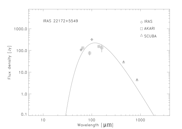
Figure 14: SED of molecular core ”A” (IRAS 22172+5549). The solid curve represents the best fit.

For a typical dust coagulation timescale $\tau_{coag}=10^{5}$ yr, in the molecular core ”A” $n_{H}\times\tau_{coag}\sim 10^{8}$ cm^-3yr$<10^{9}$ cm^-3yr, indicating that coagulation does not have a considerable effect on the dust opacity in core ”A” (Ossenkopf & Henning, 1994). Thus, the dust opacity of the initial dust distribution (without dust coagulation) with thin ice mantles can be used in the SED fitting (Ossenkopf & Henning, 1994). The dust opacity at wavelength $\lambda$ can be derived as $\kappa_{\nu}=0.797\times(\frac{\lambda}{1000\micron})^{-1.86}$, which is from fitting the data in Table 1 of Ossenkopf & Henning (1994). Figure 14 shows the SED of IRAS 22172+5549 overlaid by the best fit curve. The dust temperature from the best fit is 26.0$\pm$0.6 K, which is larger than the kinematic temperature derived from the CO emission, suggesting the dust emission traces a more innermost part than CO gas. The total mass of gas and dust traced by dust emission is 102$\pm$13 M_☉, which is much smaller than that traced by CO gas. The bolometric luminosity integrated from 20 to 3000 $\micron$ is 2200 L_☉. The dust temperature and the bolometric luminosity obtained here are consistent with the dust temperature (28$\pm$5 K) and IR luminosity (2700 L_☉) calculated using only the measured flux densities at 60 and 100 $\micron$ (Vasquez et al., 2010).

An embedded infrared cluster ”SBB1” is found in this molecular core (Saurin et al., 2010). From SED modeling, there are found to be associated with this molecular core nine YSOs younger than $5\times 10^{5}$ yr, three of which are even younger than $5\times 10^{4}$ yr, indicating that ”SBB1” is a very young star cluster. As shown in Figure 12, all nine YSOs have large infrared excesses. The three most massive ones are ”Y54”, ”Y55” and ”Y56”, which have stellar mass $\geq 6$ M_☉. The other six sources have stellar mass $\leq 3$ M_☉. The infall rate of these nine YSOs is found larger than $\sim 1\times 10^{-5}~{}M_{\sun}\cdot yr^{-1}$. ”Y57” has the largest infall rate of $\sim 1\times 10^{-3}~{}M_{\sun}\cdot yr^{-1}$. All rates indicate that young stars are forming in core ”A”.

4 Discussion

4.1 The geometry of the ring nebular

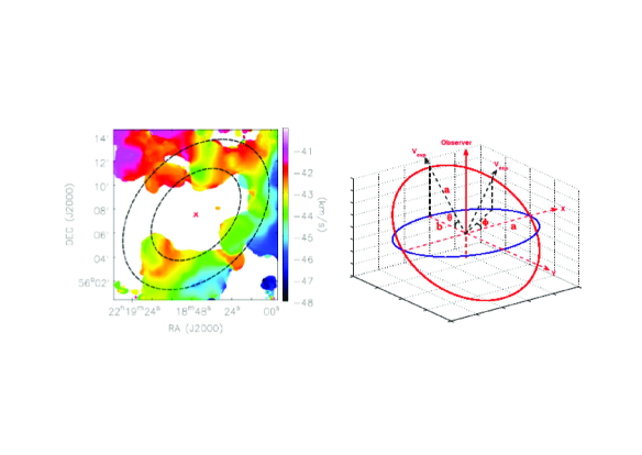
Figure 15: Left: first moment map of ¹²CO (1-0). Two ellipses are drawn for reference, to mark the boundaries of the interior and exterior of the molecular ring. Right: Coordinate system for describing the orientation in the sky of the ring nebular. The axes x and y lie on the plane of the sky. The WR star HD 211853 is located at the origin. The ring nebular is shown as a red circle. The projection of the ring nebular in the sky plane is shown as a blue ellipse. The lengths of the semimajor and semiminor axis of the ellipse are denoted as ”a” and ”b”. The angle $\theta$ is the inclination angle between the plane of the ring nebular and the sky plane. The angle $\phi$ is the position angle measured from the major axis.

The geometry of the ring nebular is important to understanding the interaction between the central Wolf-Rayet star and its environment. In this section, we argue that the molecular ring surrounding HD 211853 is more likely flattened rather than spherical. First, there is less molecular emission within the interior of the molecular ring, which excludes the spherical shell hypothesis. Second, from the first moment map of ¹²CO (1-0) in the left panel of Figure 15, one can find that the velocity distribution of the molecular gas is not spherical. The gas is redshifted and blueshifted in the north-east and south-west, respectively. But the gas along the NW-SE direction is much less shifted, indicating that the molecular gas is distributed in a ring with a thickness much smaller than the size of the bubble. The plane in which the molecular ring lies has an inclination angle with respect to the sky plane, leading to the velocity gradient of the molecular gas along NE-SW direction. Finally, as shown in Figure 2, the spectrum of ¹²CO (1-0) at the position of the WR star only has one velocity component, which excludes the two expanding layer hypothesis. The geometry and the formation of molecular rings surrounding the expanding bubbles were discussed in detail by Beaumont & Williams (2010). In their interpretation, the morphology of molecular rings naturally arises if the host molecular clouds are oblate, even sheetlike, with thicknesses of a few parsecs. The central massive stars can clear out a cavity in the flattened molecular cloud and create the molecular ring surrounding them. This is only in the case of the molecular ring surrounding HD 211853.

A simple geometric model is sketched in the right panel of Figure 15. The axes x and y lie on the plane of the sky. The WR star HD 211853 is located at the origin. The ring nebular is shown as a red circle. The projection of the ring nebular in the sky plane is shown as a blue ellipse. The lengths of the semimajor and semiminor axis of the ellipse are denoted as ”a” and ”b”. The angle $\theta$ is the inclination angle between the plane of the ring nebular and the sky plane. The angle $\phi$ is the position angle (P.A.) measured from the major axis. From this simple geometric model, the inclination angle $\theta$ can be inferred from:

$$\cos\theta=\frac{b}{a}$$ (2)

The observed velocity, $V_{obs}$ of a point on the ellipse is given by:

$$V_{obs}=V_{exp}\cdot\delta\cdot\sin\theta\sqrt{\frac{1}{1+\cos^{2}\theta\cdot\cot^{2}\phi}}+V_{sys}$$ (3)

where $V_{sys}$ is the systemic velocity, $V_{exp}$ is the expanding velocity, $\delta$=1 when $0\arcdeg\leq\phi\leq 180\arcdeg$ and $\delta$=-1 when $180\arcdeg\leq\phi\leq 360\arcdeg$. The two dashed ellipses in the left panel of Figure 15 approximately mark the boundary of the interior and exterior of the molecular ring. The inner and outer ellipses are of $4\arcmin.5\times 3\arcmin$ and $7\arcmin\times 5\arcmin$ in diameter. Thus the inclination angle between the plane of the ring nebular and the sky plane turns out to be $\sim 44\arcdeg-48\arcdeg$. From the left panel of Figure 15, the maximum value of $\mid V_{obs}-V_{sys}\mid$ is found to be 3.5 km s^-1 along the direction of the minor axis, indicating an expanding velocity of $\sim 5$ km s^-1.

As shown in Figure 1, the ring nebular surrounding HD 211853 is part (shell B) of the large HII region Sh2-132. Although shell B is mainly ionized and created by HD 211853, its interaction with the other part (shell A) cannot be ignored. The formation of shell B should be affected by the expansion of shell A, especially in the west, where the molecular ring is not closed. In the above model, we did not take into account the interaction with shell A, which needs more detailed modeling. However, the simple model can roughly depict the ring structure surrounding HD 211853 and explain the spatial and velocity distribution of the molecular gas in the ring nebular.

4.2 Gravitational stability of the molecular cores

The gravitational stability of the molecular cores can be investigated by comparing their core masses with virial masses and Jeans masses. Assuming that the cloud core is a gravitationally bound isothermal sphere with uniform density and is supported solely by random motions, the virial mass M_vir can be calculated following Ungerechts et al. (2000) as following:

$$\frac{M_{vir}}{M_{\sun}}=2.10\times 10^{2}(\frac{R}{pc})(\frac{\Delta V}{km~{}s^{-1}})$$ (4)

where R is the radius of the core and $\Delta V$ is the line width of ¹³CO (1-0). The virial masses are listed in the 15th column of Table 2.

Many factors, including thermal pressure, turbulence, and magnetic field, support the gas against gravity collapse in molecular cores. Taking into account the thermal and turbulent support, the Jeans mass can be expressed as (Hennebelle & Chabrier, 2008):

$$M_{J}=a_{J}\frac{C_{s,eff}^{3}}{\sqrt{G^{3}\rho}}$$ (5)

where $a_{J}$ is a dimensionless parameter of order unity which takes into account the geometrical factor, $\rho$ is the mass density and $C_{s,eff}$ is an effective sound speed including turbulent support,

$$C_{s,eff}=[(C_{s})^{2}+(\sigma_{NT})^{2}]^{1/2}$$ (6)

where $C_{s}$ is the thermal sound speed and $\sigma_{NT}$ is the non-thermal one dimensional velocity dispersion. The thermal sound speed is related with the kinematic temperature as following: $C_{s}=(kT_{k}/\mu_{g}m_{H_{2}})^{1/2}$, where $\mu_{g}$=1.36 is the mean atomic weight of the gas. The non-thermal one dimensional velocity dispersion $\sigma_{NT}$ can be calculated as follows:

$$\sigma_{NT}=\sqrt{\sigma_{{}^{13}CO}^{2}-\frac{kT_{k}}{m_{{}^{13}CO}}}$$ (7)

and

$$\sigma_{{}^{13}CO}=\frac{\Delta V}{\sqrt{8ln(2)}}$$ (8)

with $m_{{}^{13}CO}$ being the mass of ${}^{13}CO$. By introducing an effective kinematic temperature $T_{eff}=\frac{C_{s,eff}^{2}\mu_{g}m_{H_{2}}}{k}$, equation (5) can be rewritten in a form similar to Equation (18) in Hennebelle & Chabrier (2008),

$$M_{J}\approx 1.0a_{J}(\frac{T_{eff}}{10~{}K})^{3/2}(\frac{\mu}{2.33})^{-1/2}(\frac{n}{10^{4}~{}cm^{-3}})^{-1/2}M_{\sun}$$ (9)

where n is the volume density of H₂ calculated with RADEX, and $\mu$ is the mean molecular weight of the gas. The Jeans masses calculated are listed in the 16th column of Table 2.

The core masses of cores ”C”, ”E”, and ”H” are found to be much smaller than their viral masses and Jeans masses, while the core masses of the other cores are comparable with their virial masses and Jeans masses. Keeping this in mind, we did not consider the external pressure from their ionized boundary layers in calculating the virial masses and Jeans masses above. It seems that these cores are gravitationally stable against collapse without external pressure. However, the rising external pressure surrounding them can significantly change their stabilities and induce collapse in them (Thompson et al., 2004). The external pressure from the ionized layer is (Morgan et al., 2004):

$$\frac{P_{ext}}{k}=2\rho_{i}C_{i}^{2}=4n_{e}T_{e}$$ (10)

The effective electron temperature $T_{e}$ is assumed to be 8000 K. The electron densities $n_{e}$ in the ionized boundary layers surrounding cores ”A”, ”B”, and ”G” are taken as the values of NVSS sources 5, 4, and 1, respectively. For the other cores, we assume $n_{e}$ to be 20 cm^-3 (Vasquez et al., 2010). The calculated external pressure from the ionized layers can be found in the 18th column in Table 2. Molecular pressure inside the clouds can be expressed as:

$$\frac{P_{mol}}{k}=nT_{eff}$$ (11)

The inferred $P_{mol}$ can be found in the last column of Table 2. We can see for all the cores that external pressure from the surrounding ionized gas is much greater than the molecular pressure, indicating that the photoionization-induced shocks can penetrate the interiors of the molecular cores and compress materials inside (Morgan et al., 2004). To explore the stabilities of these cores subject to non-negligible external pressure, we calculated the ”pressurized virial mass” as (Thompson et al., 2004):

$$M_{pv}\simeq 5.8\times 10^{-2}\frac{(\Delta V)^{4}}{G^{3/2}P_{ext}^{1/2}}$$ (12)

where G is the gravitational constant and $\Delta V$ is the line width of ¹³CO (1-0) lines. The calculated ”pressurised virial masses” are listed in the 17th column of Table 2. The molecular cores with core masses exceeding their ”pressurized virial masses” are unstable against gravitational collapse (Thompson et al., 2004). Core ”C”, ”E” and ”H” have core masses smaller than their ”pressurized virial masses”, indicating they are stable even under external pressure. For the other cores, their core masses are much larger than their ”pressurized virial masses”, suggesting that they are likely to be unstable against collapse. It can be seen the high external pressure has a great destabilizing effect upon the gravitational stabilities of the cores.

4.3 The effect of the Wolf-Rayet star on the molecular distribution

It is expected that the current WR stars and their previous main sequence phases should greatly influence their associated clouds. Vasquez et al. (2010) has demonstrated that the mechanical energy released by the Wolf-Rayet star HD 211853 can shape the ring-like structure of the molecular and PAH distributions.

From Equation (3), one can see that the gases distributed along a direction of a given P.A. should have the same observed velocity. However, this is not true in the first moment map in the left panel of Figure 15. Instead, one can notice that the expanding velocity increases with the distance from the origin, especially for the gases along the NE-SW direction. This situation can also be found in the P-V diagrams in Figure 6, where the velocity distribution shows a ”Hubble law”. Such a velocity gradient was also noticed in the molecular clouds surrounding O stars (Dent et al., 2009). It seems that the expansion of the ionized gas can constantly accelerate the molecular gas. However, the acceleration is not significant toward the dense cores as shown in Figure 8. The dense molecular cores seem to have slight velocity deviation from the systemic velocity, which can be explained by the fact that the expansion of the ionized gas is decelerated by the resistance of the dense cores due to their large column densities. HD 211853 has a significant effect on its surrounding molecular gas by sweeping, photodissociating, reshaping and possibly collecting.

We also noticed that the infrared point sources in the molecular ring are always separated from the molecular cores. This effect is more significant toward cores ”C” and ”F”, where the infrared sources are located in front of the molecular core and face the central Wolf-Rayet system, indicating that the molecular cores have different expanding velocities with the infrared point sources. This separation indicates that stellar wind has different effects on the dust and gas. However, such separation maybe caused by the separation of the formed stars from their parent clouds during evolution or by inducing new cores by those formed stars. Detailed analysis and observations are needed to settle this problem.

4.4 Sequential star formation in the vicinity of core ”A”

4.4.1 Large-Scale sequential star formation

YSOs with various ages are drawn with different markers in Figure 16 overlaid on the column density of H₂ in gray scale and excitation temperature of ¹²CO (1-0) in contours. The interesting thing is that the age gradient of the YSOs appears in a large-scale. The oldest YSOs with ages larger than $2\times 10^{6}$ yr are scatted in a large area from the Wolf-Rayet system to the molecular ring. The younger ones with ages greater than 5$\times 10^{5}$ yr but smaller than 10⁶ yr are located in the midway, while the youngest ones are found associated with molecular core ”A”. Such an age gradient can also be identified in panel (i) of Figure 2 in Qiu et al. (2008). In their paper, the evolutionary stages of the YSOs in this region are identified in color-color diagrams.

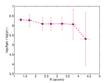
Figure 17: Distribution of $0\arcmin.5$ bin averaged ages of YSOs located between HD 211853 and core ”A” as a function of radii from the WR star. The errorbars represent the standard deviation in each bin.

We averaged the ages of the YSOs in each 0$\arcmin$.5 radius bin and present the radial age distribution in Figure 17. The projection effect was not taken into account. Since the YSOs are mainly distributed in the vicinity of core ”A”, the projection effect should not greatly affect the trend of the age distribution. We find that the YSOs within 2$\arcmin$ from the Wolf-Rayet system are as old as 2$\times 10^{6}$ yr. Those between 2$\arcmin$ and 4$\arcmin$ are aged $\sim 1.2\times 10^{6}$ yr. The youngest stars are beyond 4$\arcmin$ and have an average age of $\sim 2\times 10^{5}$ yr. It is clear that the nearer YSOs are older than the farther ones, indicating a stellar age gradient. The stellar age distribution suggests that at least three generations of stars have been forming in this region. The oldest generation is closer to the Wolf-Rayet system, while the youngest one is located in the molecular ring. In addition, the three star clusters in this region have different ages (Saurin et al., 2010). The ”Teutsch 127”, which includes the O-type star BD+55$\arcdeg$2722 and near the Wolf-Rayet star HD 211853, is the oldest one ($\sim$5 Myr). The ”SBB 2” is as old as $\sim$2 Myr. The age of the youngest cluster ”SBB 1” is about 1 Myr. The age gradient of these three star cluster also indicates sequential star formation on a large scale. Such ”relay star formation” hints at trigged star formation due to the expansion of bubbles created by stellar wind of massive stars (Chen et al., 2007).

4.4.2 Small-Scale sequential star formation

As shown in Figure 16, a small-scale age gradient is found to be associated with molecular core ”A,” a bright rimmed cloud. The older and less massive YSOs embrace the molecular core, while the youngest and more massive stars reside deeper in the core. This picture is in accordance with the so-called ”radiation-driven implosion” (RDI) process as depicted in Figure 1 of Ogura (2006), which is proposed for triggered star formation in a bright rimmed cloud (Bertoldi, 1989; Bertoldi & McKee, 1990). In the model, the surface layer of the cloud is ionized by the UV photons from massive stars and then the cloud is compressed and collapsed due to the shock generated from the ionization front. As discussed in Section 4.2, core ”A” is likely to collapse due to external pressure from the ionized boundary layer. Recent simulation suggests that there is a range of ionizing fluxes in the RDI model, that trigger star formation in the bright rimmed cloud (Bisbas et al., 2011). This range is about $10^{9}$cm^-2s${}^{-1}\lesssim\Phi_{LyC}\lesssim 3\times 10^{11}$cm^-2s^-1. If the ionizing flux is larger than $10^{9}$cm^-2s^-1, the shock front preceding the D-type ionization front can propagate into the cloud, compress it, and trigger star formation therein (Bisbas et al., 2011). However large ionizing flux can rapidly disperse the cloud without triggering star formation (Bisbas et al., 2011). The ionizing fluxes surrounding core ”A” can be estimated as (Morgan et al., 2004):

$$\Phi_{LyC}=1.24\times 10^{10}S_{\nu}T_{e}^{0.35}\nu^{0.1}\theta^{-2}$$ (13)

where $S_{\nu}$ is the integrated radio flux in mJy, $T_{e}$ is the effective electron temperature of the ionized gas in K, $\nu$ is the frequency in GHz and $\theta$ is the angular diameter over which the emission is integrated in arcseconds. Assuming $T_{e}=8000$ K, the ionizing flux in NVSS 5 is inferred as $1.1\times 10^{10}$cm^-2s^-1, which is taken as the value in the ionizing boundary layer surrounding core ”A”. This value is moderate, indicating that triggered star formation can take place in core ”A”. In the simulation of Bisbas et al. (2011), however, the RDI model favors the formation of low mass stars in the clouds, which contradicts the situation in core ”A”, where YSOs with masses larger than 6 M_☉ are found. We noticed that the initial cloud mass in their simulation is much smaller than the mass of the core ”A”, which may be responsible for the contradiction. Additionally, other processes such as ”collect and collapse” may also play important roles in star formation in core ”A”, which will be discussed in the next section.

4.5 Collect and Collapse scenario

The ring-like structure of dust and gas distribution and the existence of PDR indicate that the star formation in this region favors the ”collect and collapse” scenario (Deharveng, Zavagno, & Caplan, 2005; Vasquez et al., 2010). The molecular ring is composed of well separated, dense and massive cores, most of which are collapsing. Such regular spacing rule of the cores could not be pre-existing clumps but are formed by external triggering, which is a strong evidence for the ”collect and collapse” process (Deharveng, Zavagno, & Caplan, 2005; Ogura, 2010). This situation contradicts the RDI model, in which the dense clumps into which the radiatively induced shocks drive are pre-existing. Additionally, the large scale sequential star formation discussed in Section 4.4.1 also favors the ”collect and collapse” process rather than the ”RDI” model (Elmegreen & Lada, 1977; Ogura, 2010).

However, as discussed in Section 4.4.2, the bright rimmed nebular core ”A” also seems to favor the ”RDI” model. The ”collect and collapse” process and the ”Radiation Driven Implosion” process cannot take place at the same time and place. To resolve this contradiction, we propose that these two processes may function at different times in this region. First, neutral materials are collected and accumulated into a dense shell between the ionization front (IF) and shock front (SF) generated by the expanding HII region. Second, the compressed shocked layer becomes gravitationally unstable and fragments into regularly spaced massive clumps on a long timescale. These two steps mirror the ”collect and collapse” process. Third, the clumps are illuminated and eroded by the ionization front, leading to the formation of bright rims and/or cometary globules that collapse to form stars due to the external pressure as discussed in Section 4.2. This third step is like the ”RDI” process. Besides, the ionization front illuminating the bright rimmed nebular core ”A” is more likely generated from young cluster ”SBB 2” rather than from the central Wolf-Rayet star (Saurin et al., 2010). Relatively speaking, core ”A” is pre-existing compared with the ionization front generated from the older cluster. In addition, a possible bow-shock seems to have been generated in the cluster ”SBB 2” and seems to have an impact on ”SBB 1” (Saurin et al., 2010). We therefore suggest that the star formation in core ”A” may also be affected by the older cluster ”SBB 2” through a process like ”RDI”, leading to the formation of the youngest embedded star cluster ”SBB 1”.

4.6 Comparison with the other star forming regions

It is necessary to compare the characteristics of the molecular cores in this region with those of the other star forming regions. The line width of ¹³CO (1-0) ranges from 1.3 to 2.6 km s^-1 with a mean value of 2.1 km s^-1, which is very similar to that of the intermediate-mass star forming regions ($\sim$2 km s^-1) (Liu et al., 2011; Sun et al., 2006). It is larger than that of the low-mass star forming regions ($\sim$1.3 km s^-1) (Myers, Linke & Benson, 1983), but much smaller than that of the high-mass star forming regions associated with IRAS sources ($>$ 3 km s^-1) (Wang et al., 2009; Wu et al., 2003, 2001) or methanal masers ($\sim$4.5 km s^-1) (Liu et al., 2010). Judging from the line width of ¹³CO (1-0) in this region, the molecular cores where the triggered star formations possibly take place favor formation of intermediate-mass YSOs, which is confirmed by SED modeling of the YSOs in molecular core A. As discussed in Section 4.4.2, core A is suggested to suffer an RDI process. A tendency toward HAeBe stars forming deeper in the cloud is expected in RDI model (Ogura, 2006; Chen et al., 2007). Liu et al. (2011) found that the regions harboring HAeBe stars younger than 10⁶ yr have an average column density of $\sim 5\times 10^{21}$ cm^-2, slightly smaller than that in most cores of this region. They also have an average excitation temperature of $\sim$16 K in those HAeBe regions younger than 10⁶ yr, which is slightly lower than that of the molecular cores of this region ($\sim$20 K), indicating the influence of external heating.

5 Summary

We studied the environment surrounding Wolf-Rayet star HD 211853 in molecular, infrared, radio and HI emission. The SEDs of the YSOs that are located in the south-east part of this region are modeled with an online YSO SED fitting tool. The triggered star formation is discussed. The main findings of this paper are as follows:

(1). The molecular emission has two components. One peaks at $-50$ km s^-1, which is likely from a foreground cold cloud. The other one has a systemic velocity of $-43.5$ km s^-1, whose ¹³CO (1-0) emission forms a ring-like structure with several well separated molecular cores. The line width of ¹³CO (1-0) ranges from 1.3 to 2.6 km s^-1 with a mean value of 2.1 km s^-1, which is very similar to that of intermediate-mass star forming regions.

(2). The properties of the molecular cores are analyzed under the LTE assumption as well as with non-LTE models in RADEX. Both LTE and non-LTE analysis give the same excitation temperatures for ¹²CO (1-0) ($\sim$20 K). The excitation temperatures of ¹³CO (1-0) calculated with RADEX are much smaller than those of ¹²CO (1-0). The core masses calculated under LTE and non-LTE are similar, ranging from $\sim 10^{2}$ to $\sim 10^{3}$ M_☉. The volume densities of H₂ in this cores are $\sim 10^{3}$ cm^-3.

(3). The molecular emission is associated with 8.3$\micron$ emission in the MSX A band. We also witnessed structures like cavities and shells in HI emission. Radio emission at 1.4 GHz is embraced by the molecular and dust ring. Ionization fronts easily can be identified between the radio and molecular emission especially in the south-east part.

(4). We find that the molecular gas surrounding HD 211853 is not spherically expanding. The molecular gas distributes in a ring-like structure with a thickness much smaller than the size of the bubble. The inclination angle between the plane of the ring nebular and the sky plane turns out to be $\sim 44\arcdeg-48\arcdeg$. The expanding velocity of the ring nebular is about $\sim 5$ km s^-1. The expanding velocity seems to increase with the distance from the WR star.

(5). The molecular cores are well separated along the ring. It seems that these cores are gravitationally stable against collapse without external pressure. However the high external pressure from the ionized gas has a great destabilizing effect upon the gravitational stabilities of the cores. Core ”C”, ”E” and ”H” have core masses smaller than their ”pressurized virial masses”, indicating that they are stable even under external pressure. For the other cores, their core masses are much larger than their ”pressurized virial masses”, suggesting that they are likely to be unstable against collapse.

(5). From the SED modeling of the YSOs located in the south-east of HD 211853, a stellar age gradient is found across a large scale in space from the Wolf-Rayet star to the molecular ring. The presence of PDR, the fragmentation of the molecular ring, the collapse of the cores, and the large scale sequential star formation indicate that the ”collect and collapse” process can work in this region.

(6). Molecular core ”A” is forming a star cluster as young as $\sim 10^{5}$ yr. Core ”A” is embraced by the ionization front and older less massive YSOs. More massive YSOs are forming deeper in core A. The ionizing flux from the ionized boundary layer surrounding core ”A” is moderate enough to generate a leading shock, which propagates into the cloud, compresses it, and triggers star formation therein. This is very similar to the picture depicted by the ”Radiation-Driven Implosion” models.

In conclusion, star formation in the molecular ring is induced by the Wolf-Rayet star HD 211853 through the interaction between the expanding ionizing gas and the ISM. The evolution of the molecular ring and the triggered star formation may be affected by both the ”collect and collapse” and the ”Radiation-Driven Implosion” processes. Generally speaking, the materials in the host molecular cloud surrounding the WR star are collected into a molecular ring. Then the ring fragments into well separated cores that favor the ”collect and collapse” process. The cores are unstable due to the external pressure and collapse inside to form stars. The ionization front proceeded by a shock front generated from the older star cluster (like ”SBB 2”) can propagate into the cloud (core ”A”) and compress it and trigger star formations therein as depicted by the ”radiation-driven implosion” process.

Figure 1: Composite color image in this region: DSS2-R optical emission is blue, 1420 GHz radio emission detected in CGPS is green, and 8.3 $\micron$ emission detected at MSX A band is red. The larger ”star” shows the location of the WR star HD 211853 and the small ”star” represents the position of the massive O-type star BD+55$\arcdeg$2722. The yellow dashed ”box” shows the region of shell B, on which we focus in this paper.

Figure 6: P-V diagrams of ¹²CO (1-0) cut along the orientations denoted in Figure 7. The contours are from 0.6 K (3$\sigma$) in steps of 1 K.

Figure 8: Spectra of ¹²CO (1-0) are red, those of ¹³CO (1-0) are green and those of C¹⁸O (1-0) are blue. The core names are labeled on the upper-left corners of each panel. The dashed black lines indicate the systemic velocity of -43.5 km s^-1.

Figure 10: Upper: NVSS 1.4 GHz emission is shown in green dashed contours (0.45 mJy (1 $\sigma$) $\times$ 3,6,9,…), MSX A band emission is shown in red solid contours (from 10% to 90%), and HI emission integrated from -48 km s^-1 to -39 km s^-1 is in gray scale. Lower: NVSS 1.4 GHz emission is shown in green dashed contours, SCUBA 850 $\micron$ emission is in red solid contours (from 10% to 90%) and IRAC 8 $\micron$ emission is in color scale.

Figure 12: First nine panels present SEDs of the YSOs associated with core A. The filled circles represent the observed points. The black solid line represents the best fit to the data, while the gray solid lines represent the fits with $\chi^{2}-\chi_{best}^{2}<3\times n_{data}$, where $n_{data}$ is the number of data points. The dashed lines represent photospheric contributions, including the effect of foreground extinction. The last panel shows the SED of Y27, which favors a stellar photosphere fit rather than a YSO SED fit.

Figure 13: Comparison of the stellar mass and age of the YSOs in two runnings of the SED modeling. Left: Age comparison; Right: Mass comparison. The solid lines represent the linear fits. Age_1 and Mass_1 are the stellar age and mass obtained in the first running by exploring A_V in [2,2.5] mag. Age_2 and Mass_2 are the stellar age and mass obtained in the second running by exploring A_v in [0,2.5] mag.

Figure 16: T_ex in contours overlaid on the column density of H₂ in gray scale. The contour levels are from 20% to 90% of the peak (24 K). The young stars in different age intervals are denoted as different markers on the plot as shown in the lower-left corner. The upper age of each interval is shown in the lower-left corner. The nine YSOs associated with core ”A” are shown as color markers. The three most massive YSOs are shown as markers with red edges. The other six less massive ones are presented as markers with blue edges.

Table 1: Observed parameters of ¹³CO cores

Core	RA (J2000)	DEC (J2000)	R	Vlsr	TA(13CO)	$\Delta$V(13CO)	TA(12CO)	$\Delta$v(12CO)
	(h m s)	($\arcdeg~{}\arcmin~{}\arcsec$)	(pc)	(km s-1)	(K)	(km s-1)	(K)	(km s-1)
A	22:19:09.4	56:04:46.5	1.0	-43.8(0.3)	2.6(0.1)	2.4(0.2)	9.2(0.3)	3.4(0.2)
B	22:18:38.4	56:03:25.4	1.4	-44.2(0.1)	2.2(0.1)	2.2(0.1)	7.5(0.1)	2.7(0.2)
C	22:18:20.1	56:06:00	0.9	-43.7(0.2)	1.2(0.1)	2.5(0.1)	8.5(0.2)	2.6(0.1)
D	22:18:03.1	56:08:07.6	1.0	-43.3(0.2)	2.5(0.1)	1.7(0.2)	7.6(0.3)	2.6(0.2)
E	22:18:03.1	56:05:42.7	0.8	-46.1(0.2)	1.8(0.2)	2.0(0.2)	7.9(0.2)	2.5(0.2)
F	22:18:08.8	56:11:17.3	1.1	-42.7(0.1)	2.1(0.2)	1.9(0.2)	7.7(0.3)	2.8(0.2)
G	22:18:39.1	56:11:17.3	1.3	-43.3(0.1)	2.9(0.1)	2.6(0.2)	10.1(0.2)	3.5(0.1)
H	22:19:26.6	56:11:17.3	0.5	-42.0(0.1)	1.0(0.1)	1.3(0.2)	3.7(0.2)	2.1(0.1)
I	22:18:17.6	56:12:23.4	1.0	-50.1(0.1)	1.4(0.1)	1.1(0.1)	4.9(0.1)	1.6(0.1)

Table 2: Derived parameters of ¹³CO cores

	LTE					non-LTE
Core	$\tau$ (13CO)	Tex	N${}_{H_{2}}$	n${}_{H_{2}}$	Mcore		Tkin	N${}_{H_{2}}$	n${}_{H_{2}}$	Tex (12CO)	$\tau$ (12CO)	Tex (13CO)	$\tau$ (13CO)	Mcore	Mvir	MJ	Mpv	Pext / k	Pmol / k
		(K)	(1021 cm-2)	(103 cm-3)	(M☉)		(K)	(1021 cm-2)	(103 cm-3)	(K)		(K)		(M☉)	(M☉)	(M☉)	(M☉)	(106 cm-3K)	(105 cm-3K)
A	0.3	22	10.9	1.8	501		24.0(0.8)	9.0(0.4)	1.4(0.1)	21.7(0.5)	10.6(0.8)	15.6(0.5)	0.5	410(22)	504	544	199	5.8	5.1
B	0.3	18.5	7.3	0.8	661		20.4(0.3)	7.8(0.3)	0.9	18.5(0.2)	15.6(0.7)	10.8(0.2)	0.9	701(30)	647	523	174	3.8	2.8
C	0.2	20.5	5.2	0.9	193		26.5(1.1)	3.9(0.2)	0.7	20.5(0.4)	7.1(0.5)	9.9(0.4)	0.5	145(10)	473	870	703	0.6	2.8
D	0.3	17.8	7.0	1.1	322		20.4(0.9)	6.9(0.3)	1.1(0.1)	18.6(0.5)	14.3(1.2)	12.2(0.3)	0.8	319(16)	357	232	150	0.6	2.1
E	0.2	19	4.3	0.9	127		22.1(0.8)	5.0(0.5)	1.0(0.1)	19.3(0.4)	10.3(1.1)	11.6(0.6)	0.6	149(16)	336	383	288	0.6	2.6
F	0.3	18.8	6.4	0.9	356		21.7(1.0)	6.1(0.6)	0.9(0.1)	18.9(0.5)	11.5(1.2)	11.1(0.5)	0.8	339(323)	439	350	235	0.6	2.1
G	0.3	23.6	13.7	1.7	1061		26.2(0.6)	11.3(0.4)	1.4(0.1)	23.6(0.4)	11.2(0.6)	16.7(0.4)	0.6	877(36)	710	687	631	1.1	6.0
H	0.3	11.2	1.8	0.6	21		11.7(0.6)	2.4(0.2)	0.8(0.1)	10.8(0.4)	15.8(1.9)	6.5(0.2)	0.9	27(3)	137	121	51	0.6	0.9
I	0.3	13.2	2.2	0.3	99		14.6(0.3)	3.2(0.2)	0.5	13.2(0.2)	19.9(1.2)	7.0(0.2)	1.3	149(10)	231	103	27	0.6	0.4

Table 3: Parameters of NVSS radio sources

Number	name	RA (J2000)	DEC (J2000)	S1.4	a	b	$\theta_{R}$	ne	EM	MHII
		(h m s)	($\arcdeg~{}\arcmin~{}\arcsec$)	(mJy)	($\arcsec$)	($\arcsec$)	($\arcmin$)	(cm-3)	(pc cm-6)	(M☉)
1	221840+560824	22:18:40.77	+56:08:24.1	32.9$\pm$4.1	125.9	110.0	1.0	34	1322	1.6
2	221846+560534	22:18:46.86	+56:05:34.6	4.0$\pm$0.5	$<$80.5	$<$43.7	$<$0.5	$<$33	$<$633	$<$0.2
3	221856+560954	22:18:56.55	+56:09:54.6	20.3$\pm$2.5	83.7	65.7	0.6	54	2055	0.6
4	221852+560404	22:18:52.33	+56:04:04.0	103.4$\pm$4.1	103.0	56.1	0.6	117	9961	1.5
5	221905+560442	22:19:05.13	+56:04:42.5	87.6$\pm$3.4	98.6	29.3	0.4	181	16879	0.8
6	221826+561307	22:18:26.97	+56:13:07.7	10.0$\pm$1.4	71.7	$<$50.6	$<$0.5	$<$52	$<$1534	$<$0.3
7	221900+560045	22:19:00.72	+56:00:45.0	18.0$\pm$1.8	52.4	47.5	0.4	92	4026	0.3
8	221929+561202	22:19:29.67	+56:12:02.9	15.2$\pm$1.0	27.5	$<$31.8	$<$0.2	$<$185	$<$9675	$<$0.1
9	221912+560045	22:19:12.79	+56:00:45.0	38.2$\pm$2.7	83.2	64.5	0.6	75	3962	0.9

Table 4: The SED fitting results of the YSOs.

Name	RA (J2000)	DEC (J2000)	Number	$\chi^{2}$	log(d)	Aν	log(Age)	M∗	L∗	log(Menv)	log($\dot{M}_{env}$)	log(M${}_{disk})$	log($\dot{M}_{disk}$)	Stage
	(h m s)	($\arcdeg~{}\arcmin~{}\arcsec$)			log(kpc)	(mag)	log(yr)	M☉	L☉	log(M☉)	log(M☉yr-1)	log(M☉)	log(M☉yr-1)
Y1	22:18:45.18	+56:04:49.3	35	20.8(1.5)	0.48	2.33(0.04)	6.07(0.08)	1.54(0.20)	8(2)	-1.36(0.42)	-5.72(0.35)	-1.90(0.11)	-7.13(0.11)	0/I
Y2	22:18:45.73	+56:03:52.6	100	12.3(1.0)	0.48(0.01)	2.29(0.06)	5.43(0.45)	1.18(0.26)	20(9)	-0.62(0.34)	-5.02(0.15)	-1.76(0.22)	-6.20(0.41)	0/I
Y3	22:18:46.31	+56:05:03.4	306	10.5(0.8)	0.47(0.01)	2.26(0.07)	5.88(0.24)	0.44(0.14)	1	-2.00(0.32)	-5.93(0.31)	-2.83(0.29)	-8.56(0.39)	0/I
Y4	22:18:47.26	+56:05:58.4	37	12.6(1.7)	0.47(0.01)	2.28(0.06)	5.40(0.10)	2.08(0.36)	37(18)	-0.56(0.26)	-4.71(0.34)	-1.95(0.27)	-6.68(0.31)	0/I
Y5	22:18:47.54	+56:05:11.2	107	8.0(1.1)	0.47(0.01)	2.27(0.08)	5.95(0.33)	0.24(0.07)	1	-1.26(0.62)	-5.48(0.37)	-2.52(0.20)	-7.64(0.42)	0/I
Y6	22:18:48.01	+56:05:02.9	1	58.1	0.46	2.00	5.18	1.98	31	-1.08	-4.74	-1.35	-6.75	0/I
Y7	22:18:49.37	+56:05:46.5	1	130.1	0.46	2.46	5.54	1.30	17	-1.11	-5.75	-1.20	-5.88	0/I
Y8	22:18:49.40	+56:04:31.0	1172	5.6(1.4)	0.47(0.01)	2.28(0.10)	5.86(0.42)	0.47(0.28)	4(7)	-0.61(1.36)	-4.94(1.00)	-2.36(0.54)	-7.25(0.97)	0/I
Y9	22:18:49.86	+56:06:18.5	879	14.3(0.6)	0.48(0.01)	2.25(0.06)	6.26(0.12)	1.04(0.16)	2(1)	-2.05(0.65)	-6.14(0.58)	-2.59(0.31)	-8.22(0.82)	III
Y10	22:18:50.13	+56:03:40.8	24	11.7(1.8)	0.47(0.01)	2.20(0.06)	6.29(0.18)	2.41(0.35)	28(8)	-0.73(0.28)	-4.99(0.24)	-1.49(0.17)	-6.69(0.31)	0/I
Y11	22:18:50.78	+56:05:06.8	835	5.1(1.4)	0.48(0.01)	2.26(0.10)	6.12(0.29)	0.52(0.19)	1(1)	-1.77(0.60)	-5.79(0.54)	-2.66(0.33)	-8.01(0.64)	0/I
Y12	22:18:52.22	+56:06:13.7	306	7.4(1.1)	0.48(0.01)	2.25(0.08)	5.78(0.40)	0.55(0.25)	4(4)	-1.09(0.50)	-5.24(0.35)	-2.42(0.24)	-7.64(0.25)	0/I
Y13	22:18:52.49	+56:06:48.8	550	12.3(1.1)	0.48(0.01)	2.28(0.06)	6.06(0.16)	0.71(0.15)	2(3)	-1.34(1.35)	-5.43(1.83)	-2.37(0.28)	-7.86(1.87)	0/I
Y14	22:18:52.69	+56:06:05.1	1	30154.2	0.51	2.00	6.09	3.39	36	-2.98	-8.68	-2.20	-7.59	III
Y15	22:18:53.62	+56:06:24.8	465	15.0(1.2)	0.48(0.01)	2.34(0.05)	5.92(0.14)	0.64(0.12)	2	-1.46(0.58)	-5.63(0.42)	-2.33(0.20)	-8.14(0.24)	0/I
Y16	22:18:54.35	+56:04:59.6	81	6.9(1.3)	0.48(0.01)	2.29(0.08)	5.26(0.70)	0.42(0.14)	4(2)	-0.70(0.24)	-4.96(0.20)	-2.14(0.29)	-6.00(0.47)	0/I
Y17	22:18:55.39	+56:05:12.9	259	5.1(1.5)	0.48(0.01)	2.26(0.10)	6.12(0.30)	0.95(0.30)	3(2)	-1.06(0.78)	-5.30(0.57)	-2.40(0.30)	-7.81(0.36)	0/I
Y18	22:18:55.67	+56:05:16.3	44	7.6(1.3)	0.47(0.01)	2.22(0.07)	6.08(0.24)	1.53(0.42)	11(7)	-0.55(0.44)	-4.91(0.39)	-2.07(0.19)	-7.37(0.30)	0/I
Y19	22:18:55.67	+56:04:55.4	2584	1.7(1.9)	0.47(0.02)	2.22(0.16)	5.98(0.57)	0.36(0.28)	1(1)	-1.89(2.11)	-5.87(0.83)	-2.91(0.89)	-8.45(4.77)	0/I
Y20	22:18:56.14	+56:05:48.6	1	2131.5	0.48	2.00(0.01)	5.61	4.42	63	-1.10	-5.32	-2.86	-9.64	0/I
Y21	22:18:56.27	+56:05:32.3	894	7.1(1.2)	0.48(0.01)	2.27(0.08)	6.19(0.23)	0.83(0.25)	2(1)	-1.43(0.59)	-5.56(0.48)	-2.46(0.31)	-8.06(0.39)	0/I
Y22	22:18:57.18	+56:05:02.0	1	162.5	0.48	2.00	6.38	3.13	128	-2.63		-7.27	-13.27	III
Y23	22:18:57.62	+56:07:07.0	43	46.7(0.8)	0.48	2.32(0.03)	5.84(0.08)	1.19(0.10)	6(1)	-1.22(0.14)	-5.34(0.20)	-1.99(0.10)	-7.54(0.09)	0/I
Y24	22:18:57.71	+56:04:27.5	1084	4.5(1.7)	0.48(0.01)	2.28(0.10)	6.11(0.35)	0.45(0.24)	2(5)	-1.05(2.14)	-5.28(1.84)	-2.50(0.36)	-7.52(1.26)	0/I
Y25	22:18:57.82	+56:05:52.6	270	16.0(0.8)	0.47(0.01)	2.27(0.06)	5.34(0.47)	0.44(0.18)	5(5)	-0.42(0.65)	-4.90(0.50)	-2.29(0.39)	-6.84(1.40)	0/I
Y26	22:18:58.38	+56:04:23.3	24	15.1(1.4)	0.48	2.34(0.06)	6.88(0.04)	2.24(0.28)	46(29)	0.16(0.39)	-6.38(0.39)	-2.21(0.25)	-7.46(0.37)	III
Y27	22:18:58.68	+56:07:23.6	1	19476.0	0.51	2.50	6.11	14.60	19200	-7.86		-8.04	-9.44	III
Y28	22:18:58.71	+56:04:54.5	53	5.3(1.6)	0.48(0.01)	2.24(0.09)	5.50(0.76)	0.55(0.39)	6(8)	-0.55(0.95)	-4.99(0.75)	-2.41(0.67)	-7.32(0.35)	0/I
Y29	22:18:58.76	+56:05:18.8	1106	4.6(1.6)	0.47(0.01)	2.26(0.10)	5.55(0.38)	0.26(0.15)	1(1)	-1.61(0.67)	-5.60(0.62)	-2.85(0.42)	-8.17(1.60)	0/I
Y30	22:18:59.21	+56:05:00.6	62	2.9(2.1)	0.47(0.01)	2.27(0.10)	5.46(0.77)	0.56(0.25)	3(4)	-1.07(0.43)	-5.23(0.51)	-2.19(0.34)	-7.95(0.56)	0/I
Y31	22:18:59.72	+56:05:13.9	1	128.7	0.49	2.02	4.58	1.67	33	-0.33	-4.82	-1.24	-6.01	0/I
Y32	22:19:00.08	+56:03:14.8	314	18.4(0.7)	0.48(0.01)	2.31(0.04)	6.88(0.02)	2.36(0.06)	31(3)	-3.63(0.21)		-3.06(0.29)	-7.99(0.52)	III
Y33	22:19:00.18	+56:05:34.7	55	6.0(1.5)	0.47(0.01)	2.22(0.08)	6.01(0.36)	0.32(0.11)	2(1)	-1.17(0.39)	-5.29(0.40)	-2.35(0.21)	-7.26(0.43)	0/I
Y34	22:19:00.26	+56:06:41.4	178	4.4(1.6)	0.48(0.01)	2.22(0.09)	5.59(0.57)	0.71(0.35)	6(8)	-0.72(0.60)	-5.03(0.42)	-2.36(0.35)	-7.50(0.56)	0/I
Y35	22:19:02.01	+56:07:08.5	7	22.0(1.2)	0.47	2.15(0.04)	6.43(0.09)	2.30(0.11)	12(2)	-1.65(0.23)	-5.96(0.24)	-1.85(0.19)	-7.75(0.24)	0/I
Y36	22:19:02.01	+56:08:00.7	1391	7.8(1.1)	0.48(0.01)	2.27(0.08)	5.85(0.33)	0.34(0.16)	1(2)	-1.32(1.17)	-5.48(1.20)	-2.64(0.34)	-7.68(1.05)	0/I
Y37	22:19:02.18	+56:07:25.8	1174	3.7(1.7)	0.48(0.01)	2.28(0.11)	5.98(0.41)	0.65(0.33)	2(2)	-1.25(0.74)	-5.41(0.61)	-2.44(0.37)	-7.78(0.39)	0/I
Y38	22:19:02.26	+56:06:36.5	320	3.7(1.7)	0.48(0.01)	2.28(0.10)	6.25(0.26)	1.02(0.34)	3(2)	-1.25(1.46)	-5.58(0.97)	-2.41(0.46)	-8.06(0.43)	0/I
Y39	22:19:02.62	+56:06:17.3	706	4.2(1.7)	0.47(0.01)	2.26(0.11)	6.13(0.33)	0.44(0.25)	2(5)	-1.05(2.41)	-5.23(2.22)	-2.61(0.42)	-7.79(1.71)	0/I
Y40	22:19:02.77	+56:05:40.6	116	14.9(1.2)	0.48(0.01)	5.03(0.53)	6.27(0.12)	1.85(0.27)	20(10)	-1.25(0.60)	-5.66(0.48)	-2.27(0.18)	-8.16(0.31)	0/I
Y41	22:19:03.80	+56:05:10.3	81	12.1(1.2)	0.47(0.01)	2.27(0.06)	5.85(0.36)	0.68(0.22)	4(2)	-1.04(0.46)	-5.26(0.28)	-2.07(0.13)	-7.21(0.24)	0/I
Y42	22:19:04.36	+56:05:50.8	395	7.1(1.2)	0.48(0.01)	2.29(0.08)	5.94(0.41)	0.74(0.36)	11(12)	0.00(0.86)	-4.59(0.56)	-2.04(0.48)	-6.49(0.77)	0/I
Y43	22:19:04.46	+56:05:36.0	1	113.3	0.48	2.42	6.09	3.39	36	-2.98	-8.68	-2.20	-7.59	III
Y44	22:19:04.50	+56:05:07.8	215	6.3(1.4)	0.47(0.01)	2.26(0.09)	5.62(0.52)	0.68(0.34)	10(10)	-0.32(0.70)	-4.72(0.58)	-2.19(0.43)	-6.68(1.48)	0/I
Y45	22:19:05.21	+56:08:25.8	10	46.4(0.9)	0.49	2.31(0.03)	5.42(0.04)	0.85(0.08)	7(1)	-0.66(0.14)	-4.92(0.14)	-2.01(0.07)	-7.22(0.08)	0/I
Y46	22:19:05.72	+56:04:52.7	218	6.7(1.3)	0.48(0.01)	2.27(0.09)	5.30(0.59)	2.07(0.69)	62(37)	0.18(0.60)	-4.60(0.26)	-1.42(0.37)	-6.17(0.36)	0/I
Y47	22:19:05.79	+56:07:05.9	138	10.9(0.9)	0.48(0.01)	2.29(0.06)	5.87(0.12)	0.68(0.15)	2	-1.87(0.62)	-6.15(0.31)	-2.58(0.22)	-8.21(0.31)	III
Y48	22:19:05.82	+56:05:18.8	10	108.1(0.6)	0.47	2.29(0.02)	5.06(0.03)	2.51(0.19)	74(13)	0.72(0.06)	-4.08(0.04)	-2.22(0.04)	-7.37(0.08)	0/I
Y49	22:19:05.94	+56:05:41.7	262	4.9(1.6)	0.48(0.01)	2.27(0.09)	5.89(0.31)	0.71(0.31)	5(8)	-0.74(0.95)	-4.83(1.21)	-2.45(0.75)	-7.32(2.15)	0/I
Y50	22:19:06.02	+56:05:55.3	1	41.0	0.51	2.00	5.77	3.58	24	-1.46	-5.25	-5.07	-10.84	0/I
Y51	22:19:07.65	+56:05:28.6	22	14.5(1.6)	0.48(0.01)	2.23(0.06)	5.68(0.30)	3.09(0.40)	67(25)	-0.42(0.13)	-4.60(0.15)	-1.61(0.27)	-6.47(0.42)	0/I
Y52	22:19:08.03	+56:04:11.1	1	130.6	0.44	2.00	6.31	4.80	408	-5.15		-0.82	-7.62	III
Y53	22:19:08.30	+56:05:11.0	2	387.4(0.6)	0.45	2.16(0.01)	4.51(0.02)	2.93(0.03)	98(1)	0.07(0.01)	-4.41(0.01)	-1.14(0.03)	-5.57(0.03)	0/I
Y54	22:19:08.45	+56:05:28.7	72	9.4(1.8)	0.48(0.01)	2.27(0.07)	5.51(0.35)	1.28(0.43)	18(10)	0.27(0.49)	-4.42(0.27)	-1.61(0.18)	-6.42(0.17)	0/I
Y55	22:19:09.38	+56:05:00.4	1	299.6	0.46	2.50	4.12	7.72	607	1.19	-4.40	-0.92	-5.96	0/I
Y56	22:19:09.39	+56:04:45.7	1	193.3	0.44	2.00	5.20	7.24	1003	1.88	-4.04	-0.96	-7.04	0/I
Y57	22:19:09.70	+56:05:04.8	1	30.7	0.48	2.00	3.61	5.91	478	1.22	-2.92	-2.32	-6.35	0/I
Y58	22:19:09.84	+56:07:37.4	1438	4.1(1.5)	0.48(0.01)	2.27(0.11)	5.72(0.54)	0.36(0.24)	2(3)	-1.33(0.92)	-5.42(0.53)	-2.55(0.43)	-7.76(0.88)	0/I
Y59	22:19:09.94	+56:08:20.5	174	8.4(1.1)	0.48(0.01)	2.27(0.07)	5.45(0.40)	0.32(0.14)	2(2)	-1.19(0.36)	-5.28(0.25)	-2.42(0.28)	-7.33(0.52)	0/I
Y60	22:19:10.94	+56:06:07.6	1134	5.4(1.4)	0.48(0.01)	2.26(0.09)	6.24(0.23)	0.60(0.20)	1	-1.97(0.99)	-6.00(0.68)	-2.77(0.48)	-8.48(0.47)	III
Y61	22:19:12.07	+56:07:09.1	54	9.8(1.2)	0.47(0.01)	2.20(0.07)	5.76(0.18)	0.66(0.14)	3(2)	-1.12(0.36)	-5.31(0.25)	-2.28(0.37)	-7.15(0.45)	0/I
Y62	22:19:13.80	+56:07:48.4	305	15.9(1.2)	0.49(0.01)	2.82(0.42)	6.75(0.04)	2.18(0.12)	26(7)	-3.39(0.40)	-8.72(2.28)	-3.04(0.82)	-10.24(0.57)	III
Y63	22:19:15.06	+56:06:53.0	194	4.0(1.7)	0.48(0.01)	2.24(0.10)	5.92(0.47)	0.49(0.24)	1(1)	-1.62(0.89)	-5.73(0.75)	-2.49(0.48)	-8.20(0.44)	0/I
Y64	22:19:15.18	+56:07:02.8	2239	2.2(1.7)	0.47(0.02)	2.26(0.14)	6.35(0.29)	0.73(0.35)	1(2)	-1.85(13.16)	-6.11(9.52)	-2.85(0.85)	-8.51(5.91)	III

References

- Beaumont & Williams (2010) Beaumont, C. N., & Williams, J. P., 2010, 709, 791
- Bertoldi (1989) Bertoldi, F. 1989, ApJ, 346, 735
- Bertoldi & McKee (1990) Bertoldi, F. & McKee, C. F. 1990, ApJ, 354, 529
- Bisbas et al. (2011) Bisbas, T. G., Wünsch, R., Whitworth, A. P., Hubber, D. A., Walch, S., 2011, ApJ, 736, 142
- Brand et al. (2011) Brand, J., Massi, F., Zavagno, A., Deharveng, L., Lefloch, B., 2011, A&A, 527, 62
- Cappa et al. (2008) Cappa, C. E., Vasquez, J., Arnal, E. M., Cichowolski, S., Pineault, S., 2008, RMxAC, 33, 142
- Chen et al. (2007) Chen, W. P., Lee, H. T., Sanchawala, K., 2007, IAUS, 237, 278
- Condon et al. (1998) Condon, J. J., Cotton, W. D., Greisen, E. W., Yin, Q. F., Perley, R. A., et al., 1998, AJ, 115, 1693
- Dent et al. (2009) Dent, W. R. F., Hovey, G. J., Dewdney, P. E., Burgess, T. A., Willis, A. G., et al., 2009, MNRAS, 395, 1805
- Deharveng et al. (2003) Deharveng, L., Lefloch, B., Zavagno, A., Caplan, J., Whitworth, A. P., et al. 2003, A&A, 408, L25
- Deharveng, Zavagno, & Caplan (2005) Deharveng, L., Zavagno, A., & Caplan, J., 2005, A&A, 433,565
- Deharveng et al. (2008) Deharveng, L., Lefloch, B., Kurtz, S., Nadeau, D., Pomarès, M., et al., 2008, A&A, 482, 585
- Di Francesco et al. (2008) Di Francesco, J., Johnstone, D., Kirk, H., MacKenzie, T., Ledwosinska, E., 2008, ApJS, 175, 277
- Elmegreen & Lada (1977) Elmegreen, B. G., & Lada, C. J. 1977, ApJ, 214, 725
- Garden et al. (1991) Garden, R. P., Hayashi, M., Hasegawa, T., Gatley, I., Kaifu, N., 1991, ApJ, 374, 540
- Grave & Kumar (2009) Grave J. M. C. & Kumar M. S. N., 2009, A&A, 498, 147
- Gritschneder et al. (2009) Gritschneder, M., Naab, T., Burkert, A., Walch, S., Heitsch, F., et al., 2009, MNRAS, 393, 21
- Guilloteau & Lucas (2000) Guilloteau, S. & Lucas, R., 2000, in Astronomical Society of the Pacific Conference Series, Vol. 217, Imaging at Radio through Submillimeter Wavelengths, ed. J. G. Mangum & S. J. E. Radford, 299
- Harten, Felli & Tofani. (1978) Harten R. H., Felli M., Tofani G., 1978, A&A, 70, 205
- Haworth & Harries. (2012) Haworth, T. J. & Harries, T. J., 2012, MNRAS, 420, 562
- Hennebelle & Chabrier (2008) Hennebelle, P., & Chabrier, G., 2008, ApJ, 684, 395
- Hester & Desch (2005) Hester, J. J., & Desch, S. J. 2005, ASP Conf. Ser. 341: Chondrites and the Protoplanetary Disk, 341, 107
- Lefloch & Lazareff. (1994) Lefloch B, & Lazareff, B., 1994, A&A, 289, 559
- Li & Goldsmith (2003) Li, D., & Goldsmith, P. F. 2003, ApJ, 585, 823
- Liu et al. (2010) Liu, T., Wu, Y.-F., Wang, K., 2010, RAA, 10, 67
- Liu et al. (2011) Liu, T., Zhang, H. W., Wu, Y. F., Qin, S.-L., Miller, M., 2011, ApJ, 734, 22
- Marston (1996) Marston, A. P., 1996, AJ, 112, 2828
- Martín-Pintado et al. (1999) Martín-Pintado, J., Gaume, R. A., Rodríguez-Fernández, N., de Vicente, P., Wilson, T. L., 1999, ApJ, 519, 667
- Miao et al. (2009) Miao J., White G. J., Thompson M. A., Nelson R. P., 2009, ApJ, 692, 382
- Morgan et al. (2004) Morgan, L. K., Thompson, M. A., Urquhart, J. S., White, G. J., Miao, J., 2004, A&A, 426, 535
- Morgan et al. (2010) Morgan, L. K., Figura, C. C., Urquhart, J. S., Thompson, M. A., 2010, MNRAS, 408, 157
- Myers, Linke & Benson (1983) Myers, P. C., Linke, R. A., & Benson, P. J., 1983, ApJ, 264, 517
- Nishimaki et al. (2008) Nishimaki, Y., Yamamuro, T., Motohara, K., Miyata, T., Tanaka, M., 2008, PASJ, 60, 191
- Ogura (2006) Ogura, Katsuo., 2006, BASI, 34, 1110
- Ogura (2010) Ogura, K., 2010, ASInC, 1, 190
- Ossenkopf & Henning (1994) Ossenkopf, V., & Henning, T. 1994, A&A, 291, 943
- Panagia & Walmsley (1978) Panagia, N. & Walmsley, C. M., 1978, A&A, 70, 411
- Petriella et al. (2010) Petriella, A., Paron, S., & Giacani, E. 2010, A&A, 513, A44+
- Pomarès, M. et al. (2009) Pomarès, M., Zavagno, A., Deharveng, L., Cunningham, M., Jones, P., et al., 2009, A&A, 494, 987
- Price et al. (2001) Price, S. D., Egan, M. P., Carey, S. J., Mizuno, D. R., Kuchar, T. A., 2001, AJ, 121, 2819
- Qiu et al. (2008) Qiu, Keping., Zhang, Qizhou., Megeath, S. Thomas., Gutermuth, Robert A., Beuther, Henrik., et al, 2008, ApJ, 685, 1005
- Robitaille et al. (2006) Robitaille T. P., Whitney B. A., Indebetouw R., Wood K., & Denzmore P., 2006, ApJS, 167, 256
- Robitaille et al. (2007) Robitaille T. P., Whitney B. A., Indebetouw R., and Wood K., 2007, ApJS, 169, 328
- Saurin et al. (2010) Saurin, T. A., Bica, E., & Bonatto, C., 2010, MNRAS, 407, 133
- Shan et al. (2009) Shan, W., Li, Z., Zhong, J., Shi, S., 2009, IEEE Trans. On Appl. Supercond, 19, 432.
- Sharpless (1959) Sharpless S., 1959, ApJS, 4, 257
- Sugitani et al. (1991) Sugitani, K., Fukui, Y., Ogura, K., 1991, ApJS, 77, 59
- Sugitani & Ogura (1994) Sugitani, K., & Ogura, K., 1994, ApJS, 92, 163
- Sun et al. (2006) Sun, K., Kramer, C., Ossenkopf, V., Bensch, F., Stutzki, J., et al., 2006, A&A, 451, 539
- Taylor et al. (2003) Taylor, A. R., Gibson, S. J., Peracaula, M., Martin, P. G., Landecker, T. L., et al., 2003, AJ, 125, 3145
- Thompson et al. (2004) Thompson, M. A., White, G. J., Morgan, L. K., Miao, J., Fridlund, C. V. M., et al., 2004, A&A, 414, 1017
- Ungerechts et al. (2000) Ungerechts H., Umbanhowar P., & Thaddeus P., 2000, ApJ, 537, 221
- Urquhart et al. (2004) Urquhart J. S., Thompson M. A., Morgan L. K., White G. J., 2004, A&A, 428, 723
- Urquhart et al. (2006) Urquhart J. S., Thompson M. A., Morgan L. K., White G. J., 2006, A&A, 450, 625
- Urquhart et al. (2007) Urquhart J. S., Thompson M. A., Morgan L. K., Pestalozzi M. R., White G. J., Muna D. N., 2007, A&A, 467, 1125
- Van der Tak et al. (2007) Van der Tak, F.F.S., Black, J.H., Schöier, F.L., Jansen, D.J., van Dishoeck, E.F. 2007, A&A, 468, 627
- Vasquez et al. (2010) Vasquez, J., Cappa, C. E., Pineault, S., Duronea, N. U., 2010, MNRAS, 405, 1976
- Wang et al. (2009) Wang, K., Wu, Y. F., Ran, L., Yu, W. T., Miller, M., 2009, A&A, 507, 369
- Whitworth et al. (1994) Whitworth, A. P., Bhattal, A. S., Chapman, S. J., Disney, M. J., & Turner, J. A. 1994, MNRAS, 268, 291
- Wu et al. (2003) Wu, Y., Wang, J., & Wu, J., 2003, Chin. Phys. Letter, 20, 1409
- Wu et al. (2001) Wu, Y., Wu, J., Wang, J., 2001, A&A, 380, 665
- Zavagno et al. (2006) Zavagno, A., Deharveng, L., Comerón, F., Brand, J., Massi, F., et al., 2006, A&A, 446, 171
- Zavagno et al. (2007) Zavagno, A., Pomarès, M., Deharveng, L., Hosokawa, T., Russeil, D., et al., 2007, A&A, 472, 835
- Zhu et al. (2010) Zhu, L., Wright, M. C. H., Zhao, J-H., Wu, Y. F., 2010, ApJ, 712, 674